Projected changes in particulate matter concentrations in the South Coast Air Basin due to basin-wide reductions in nitrogen oxides, volatile organic compounds, and ammonia emissions

ABSTRACT

An ozone abatement strategy for the South Coast Air Basin (SoCAB) has been proposed by the South Coast Air Quality Management District (SCAQMD) and the California Air Resources Board (ARB). The proposed emissions reduction strategy is focused on the reduction of nitrogen oxide (NO_x) emissions by the year 2030. Two high PM_2.5 concentration episodes with high ammonium nitrate compositions occurring during September and November 2008 were simulated with the Community Multi-scale Air Quality model (CMAQ). All simulations were made with same meteorological files provided by the SCAQMD to allow them to be more directly compared with their previous modeling studies. Although there was an overall under-prediction bias, the CMAQ simulations were within an overall normalized mean error of 50%; a range that is considered acceptable performance for PM modeling. A range of simulations of these episodes were made to evaluate sensitivity to NO_x and ammonia emissions inputs for the future year 2030. It was found that the current ozone control strategy will reduce daily average PM_2.5 concentrations. However, the targeted NO_x reductions for ozone were not found to be optimal for reducing PM_2.5 concentrations. Ammonia emission reductions reduced PM_2.5 and this might be considered as part of a PM_2.5 control strategy.

Implications: The SCAQMD and the ARB have proposed an ozone abatement strategy for the SoCAB that focuses on NO_x emission reductions. Their strategy will affect both ozone and PM_2.5. Two episodes that occurred during September and November 2008 with high PM_2.5 concentrations and high ammonium nitrate composition were selected for simulation with different levels of nitrogen oxide and ammonia emissions for the future year 2030. It was found that the ozone control strategy will reduce maximum daily average PM_2.5 concentrations but its effect on PM_2.5 concentrations is not optimal.

Introduction

There have been several modeling studies of ozone (O₃) and particulate matter (PM) conducted for the South Coast Air Basin (SoCAB; e.g., Chen et al. 2013; Kelly et al. 2014). In contrast to these studies, the objective of the research presented here is to evaluate the effect of an ozone control strategy on particulate matter (PM) concentrations for the SoCAB.

The South Coast Air Quality Management District (SCAQMD) has set emission reduction goals for volatile organic compounds (VOC) and nitrogen oxides (NO_x = NO + NO₂) between 2008 and 2030 with the objective of reaching compliance with federal ozone standards in the SoCAB. The SCAQMD Air Quality Management Plan (South Coast Air Quality Management District [SCAQMD] 2013; 2017) is very focused on NO_x emission reductions. Fujita et al. (2016) used the Community Multi-scale Air Quality model (CMAQ; Binkowski 1999; Binkowski and Shankar 1995; Byun and Ching 1999; Byun and Schere 2006) to simulate the response of ozone concentrations to the planned emission reductions in the SoCAB between the base year 2008 and the future year 2030 (Fujita et al. 2016). In contrast to the SCAQMD Plan (2013), Fujita et al. found that an NO_x-focused ozone abatement strategy will cause higher ozone concentrations in the western and central SoCAB over a prolonged time until very large NO_x reductions are achieved.

Although the SCAQMD Air Quality Management Plan (SCAQMD 2013; 2017) focuses on ozone abatement through NO_x reductions, this strategy could affect the concentrations of other air pollutants such as PM. Fujita et al. (2016) did not examine the consequences of the emission reductions on PM because this was beyond their scope. This study is an extension of Fujita et al. (2016) with its purpose to examine the effects of the SCAQMD ozone abatement plan on PM concentrations. Given that this study extends Fujita et al. (2016), a resulting limitation is that we focus more deeply on the SCAQMD (2013) plan rather than the updated SCAQMD (2017) plan.

PM may be grouped into two categories, primary PM and secondary PM. Both of these categories include fine particulate matter with an aerodynamic diameter of 2.5 µm or less (PM_2.5). Primary PM is directly emitted into the atmosphere by emission sources. Primary PM includes black or elemental carbon, soot, and fine particles formed by combustion processes, most coarse PM (with diameters greater than 10 μm; PM₁₀), windblown crustal material, fugitive dust, and similar substances.

Primary PM concentrations are not very likely to be directly affected by changes in VOC and NO_x emissions. The lack of a direct relationship between primary PM concentrations and the emissions of VOC and NO_x makes a detailed analysis of primary PM changes beyond the scope of this research project. However, changes in direct PM emissions between 2008 and 2030 are expected (SCAQMD 2013, 2017). These changes to primary PM emissions were implemented in the emissions inventories used for the CMAQ modeling presented here.

Secondary PM is the component of PM that is formed in the atmosphere through chemical reactions. The formation of secondary PM is a highly nonlinear function of VOC and NO_x emissions. The chemistry that produces secondary PM is strongly coupled with the gas-phase chemistry of ozone formation because the oxidation products of NO_x, sulfur dioxide (SO₂), and VOC include nitric acid (HNO₃), sulfuric acid (H₂SO₄), and other products with low equilibrium vapor pressures that can partition into the aerosol phase to yield PM (Calvert et al. 2015). The atmospheric acids HNO₃ and H₂SO₄ react with ammonia (NH₃) to produce the PM_2.5 components ammonium nitrate (NH₄NO₃), ammonium bisulfate (NH₄HSO₄), and ammonium sulfate ((NH₄)₂SO₄), if sufficient NH₃ is present. These compounds are produced through oxidation reactions involving the hydroxyl radical (HO) that is central also to the chemistry of ozone formation. The composition of VOC is important because different organic compounds have different reactivity for producing ozone. Reductions in VOC and NO_x emissions affect the formation of other secondary PM components such as secondary organic aerosol (SOA). The gas-phase chemical production of PM from precursor emissions yields smaller particles that contribute to PM_2.5. PM_2.5 is of particular concern because fine particles have deleterious effects on health when inhaled (Brunekreef and Holgate 2002; Cohen et al. 2017; Grahame, Klemm, and Schlesinger 2014; Sicard et al. 2010; Stewart et al. 2017).

A reasonable expectation is that reductions in NO_x emissions would reduce the formation of secondary NH₄NO₃ aerosol. However, reductions in VOC or NO_x emissions do not always lead to lower ozone levels in the SoCAB (Fujita et al. 2016), and the same could be true for PM. For these reasons the Community Multi-scale Air Quality (CMAQ), a comprehensive air quality model, was used to evaluate the effects of the proposed ozone abatement strategy on PM_2.5.

In this paper we present an evaluation of trends in PM_2.5 concentrations and the components nitrate, sulfate, organic carbon (OC), and elemental carbon (EC) for the SoCAB. Two high PM_2.5 episodes with high NH₄NO₃ composition were selected for CMAQ modeling based on the examination of the PM measurements for the year 2008. The two 2008 episodes were simulated by CMAQ and a modeling evaluation was performed. For the 2008 episodes the effect of VOC emission inventory increases on secondary PM_2.5 were simulated. Then the effect of six NO_x and four ammonia (NH₃) emission reduction scenarios on PM_2.5 were simulated for the future year 2030. Finally, the simulation results and their implications for the effect of the proposed ozone control strategy on PM_2.5 are presented.

Measurements and trends in PM_2.5 concentrations over the SoCAB

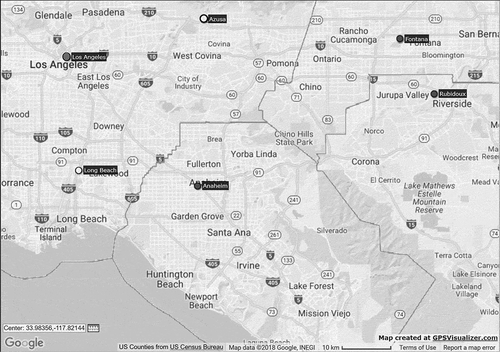
The high level of emissions due to the SoCAB’s population, its location by the Pacific Ocean, and its surrounding mountain topography make it difficult for air quality standards to be attained for ozone and PM. There is a population of 17.8 million people living in an area of 10,743 square miles in the SoCAB (Fujita et al. 2016). PM measurements made at ambient air monitoring sites operating in the SoCAB were used to update PM trends, to identify high PM episodes for CMAQ modeling, and to evaluate CMAQ model performance. Six ambient air monitoring sites operating in the SoCAB reported daily mass concentrations of PM_2.5 in 2008, with four of these stations reporting chemical speciation data as shown in Figure 1.

Figure 1. Map of the South Coast Air Basin with approximate locations of the PM_2.5 monitoring sites that reported daily mass concentration in 2008 and were used in this study. Filled dots indicate sites that also reported chemical speciation data.

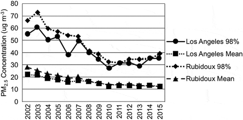
Trends in the annual mean and 98th percentile of daily PM_2.5 concentrations at the Central Los Angeles site (CELA) and Rubidoux (RUBI) sites are shown in Figure 2. The daily PM_2.5 concentrations decreased between 2002 and 2010 at Los Angeles and Rubidoux. Following 2010, the PM_2.5 concentrations level off and may have increased slightly by 2015 at Los Angeles, while at Rubidoux the PM_2.5 concentrations remained almost constant between 2010 and 2015.

Figure 2. Trend in annual mean and 98th percentile of daily PM_2.5 concentrations at the Central Los Angeles and Rubidoux sites.

Trends in chemical constituents of PM, organic carbon, elemental carbon, nitrate, and sulfate were examined. Nitrate is the chemical component with the greatest concentrations that is most likely affected by changes in VOC and NO_x emissions, as discussed in the Results section of this paper. The annual mean nitrate concentrations at the Rubidoux site were greater than those at the Los Angeles site between 2003 and 2014, as shown in Figure 3. The annual mean average nitrate concentrations at Rubidoux were near 12 μg m⁻³, while at Central Los Angeles they were near 6.5 μg m⁻³ during 2002. The annual mean nitrate concentration decreased at both sites after 2002 and the nitrate concentrations were near 4 μg m⁻³ at both Rubidoux and Central Los Angeles during 2014.

Figure 3. Trends in nitrate concentrations at the Central Los Angeles and Rubidoux sites are shown. The top plot shows the trend in the annual mean average, while the lower plot shows the nitrate contribution to the NAAQS PM_2.5 design value.

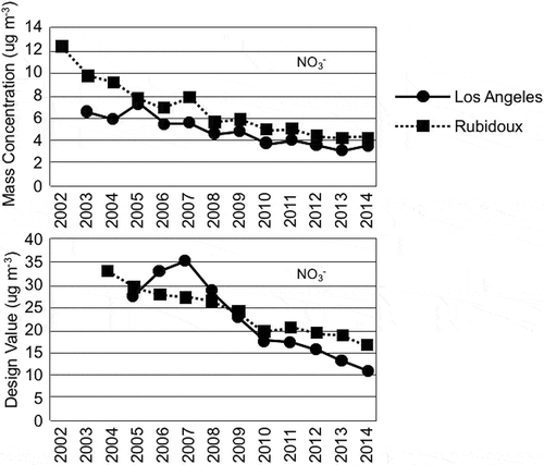
The nitrate “design values” (analogous to the design value for ozone, this is the 3-year running average of the annual 98th percentile of daily mean PM concentrations) at the two sites had similar magnitudes. The nitrate design values were in the range of 30 to near 35 μg m⁻³ at both sites near the years 2004 to 2006. The design value at the Los Angeles site increased initially and then fell from 2007 to 2014, while at the Rubidoux site the design value fell more steadily during this time. The design value at Los Angeles decreased to 37% of its initial value and the design value at Rubidoux decreased to 50% of its initial value. The nitrate design value was near 17 μg m⁻³ at Rubidoux and near 10 μg m⁻³ at Central Los Angeles during 2014.

The annual mean sulfate concentrations are significantly lower than the annual mean nitrate concentrations at Rubidoux and the Central Los Angeles sites, as shown in Figure 4. The annual mean sulfate concentrations were greater at the Central Los Angeles site than at the Rubidoux site. The mean sulfate concentrations at Central Los Angeles ranged from 3 to 4.5 μg m⁻³ during the early 2000s, while at Rubidoux they ranged from near 2.5 to 3.5 μg m⁻³ during this same time period. There was an increase in the annual mean sulfate concentration at Central Los Angeles during 2005, but there was a decrease to 44% of its initial value between 2002 and 2010. At the Rubidoux site there was a decrease in the annual mean sulfate concentration to 40% of its initial value between 2002 and 2010. By 2010 the annual mean sulfate concentration decreased to a range of 1.5 to 2.0 μg m⁻³ at both sites. There was little change in the sulfate concentrations at both sites between 2010 and 2014.

Figure 4. Trends in sulfate concentrations at the Central Los Angeles and Rubidoux sites are shown. The top plot shows the trend in the annual mean average, while the lower plot shows the sulfate contribution to the NAAQS PM_2.5 design value.

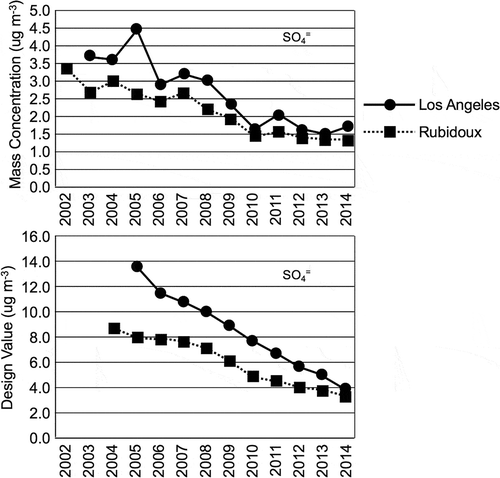
The sulfate design values were 8.5 μg m⁻³ at Rubidoux during 2004 and 13.5 μg m⁻³ at Central Los Angeles during 2005. The sulfate design values decreased steadily between 2004 and 2014 at both sites. The decrease was greatest at Los Angeles, decreasing to 27% of its initial value, compared with 39% at Rubidoux. The sulfate design values fell to near 4 μg m⁻³ at both sites by 2014. These comparisons show that the nitrate component of the aerosol is significantly larger than the sulfate component.

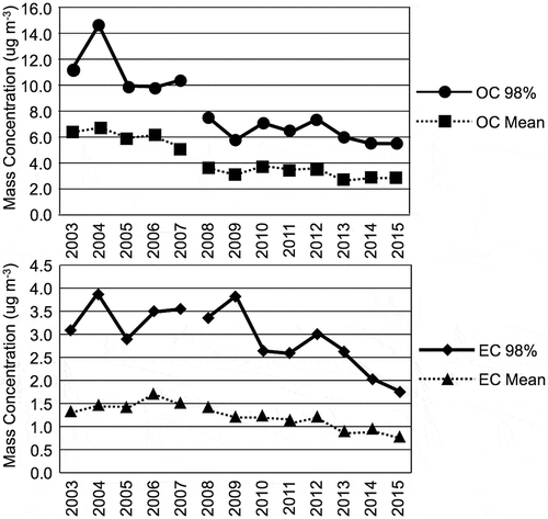
It’s more difficult to assess the relative significance of the OC and EC components of PM_2.5 found in the SoCAB relative to nitrate and sulfate. Figure 5 shows that OC at the Central Los Angeles site appears to decrease significantly from over 6 to 3 μg m⁻³ while the EC drops from a peak near 1.6 to 0.75 μg m⁻³. However, the apparent drops in OC and EC are more likely due to changes in measurement methods. The figure shows data from the Chemical Speciation Network (CSN). Changes were made to the CSN protocol for the measurement of OC and EC during 2007. The goal was to make CSN measurements more consistent with the U.S. Interagency Monitoring of PROtected Visual Environments (IMPROVE) network. The IMPROVE network implemented a new temperature protocol for its thermal methods used to measure OC and EC (Chow et al. 2007). Spada and Hyslop (2018) present a comparison of OC and EC measurements from the two networks using measurements made before and after the protocol changes. Spada and Hyslop found that the CSN protocol changes increased its measured EC and decreased measured OC mass concentrations. Therefore, it’s very likely that there has been little change in EC and OC concentrations at the Central Los Angeles site between 2003 and 2015. This data analysis shows that overall the EC and OC PM_2.5 components are not as large as the nitrate components.

Figure 5. Trend in annual mean and 98th percentile of CSN protocol organic and elemental carbon concentrations at the Central Los Angeles site. A change in the analysis method for carbon fractions was implemented in 2007, so data collected before and after 2007 may not be fully comparable.

Selection of episodes for the 2008 base year

The episodes selected for modeling had PM_2.5 concentrations with high nitrate particulate fractions during the 2008 base year. It was required that the selected 2008 episodes have chemically speciated data for model evaluation. The episodes chosen for modeling included two of the highest PM concentrations during the 2008 aerosol season. The two selected episodes had high particulate nitrate concentrations as well. This selection procedure is analogous with previously accepted EPA State Implementation Plan (SIP) modeling protocols for ozone and with other PM modeling studies (e.g. Kleeman, Ying, and Kaduwela 2005; Nguyen and Dabdub 2002). Some PM modeling studies have investigated continental domains with simulations of 1-year duration (Makar et al. 2009), and this seems necessary if the effects of very long-range transport of precursors are to be investigated, but this is not relevant for our SoCAB simulations.

Ozone SIP modeling is not usually made for average days; instead, highly polluted episodes are chosen, and this same strategy has been followed in this work. Typically for an ozone SIP, a field study is conducted, and intensive measurements are made during highly polluted events and then these are modeled. Events that are atypical, such as episodes influenced by nearby wildfires, are excluded from the process. The two episodes were modeled and analysis of these simulations showed that both led to similar conclusions. This suggests that our methodology is robust.

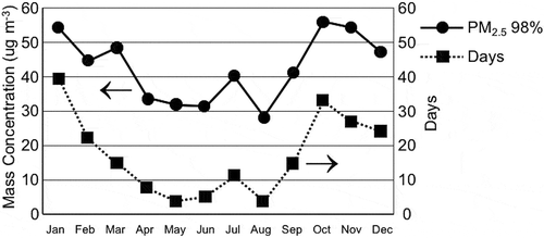
The highest daily PM_2.5 concentrations usually occur during the fall and winter seasons in the SoCAB. Figure 6 shows daily PM_2.5 concentration data statistics by month for the years between 2002 and 2015 at the Central Los Angeles site. The majority of high daily PM_2.5 concentrations occurred between September and February for these years.

Figure 6. Daily PM_2.5 concentration data by month for the years between 2002 and 2015 are shown for the Central Los Angeles site. Plotted are the 98th percentiles of the PM_2.5 concentrations (upper lines) and the number of days during the time period when the PM_2.5 concentrations were greater than 35 μg m⁻³ (lower line).

The highest two PM levels during 2008 were found to occur during the fall and winter seasons in the SoCAB. The first episode occurred from Friday September 12 to Monday September 15 with the greatest PM concentration on the 13th. The second episode occurred from Tuesday November 11 to Monday November 24. These two episodes are shown in Figures 7 and 8 and, based on the available speciation data, they were driven by high nitrate (NO₃⁻) concentrations. These two episodes were very appropriate for this modeling study because nitrate is a secondary aerosol pollutant.

Figure 7. Top panel presents a time-series plot of daily mean PM_2.5 concentrations for September 2008. The dashed-line box signifies the period selected for modeling. Lower panel presents a time-series plot of daily mean PM_2.5 concentrations for November 2008. The dashed-line box signifies the period selected for modeling.

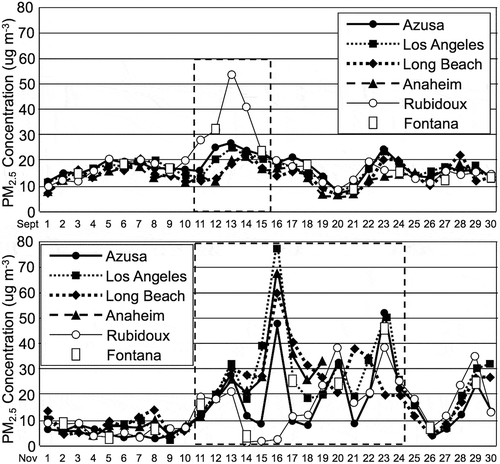
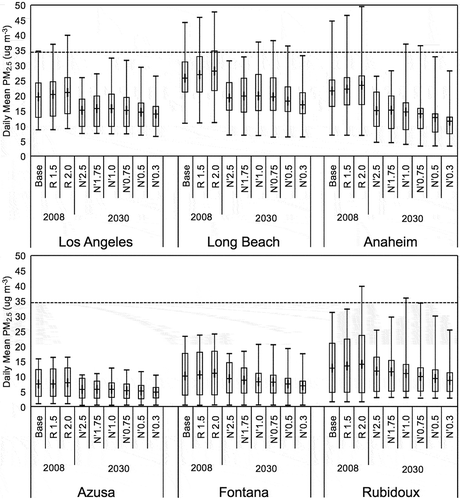
Figure 8. Range of simulated daily mean mass of PM_2.5 at six monitoring sites in the SoCAB. The adjustments to VOC emissions were made for 2008 and the adjustments to NO_x emissions were made for 2030. The box and whisker plots indicate the minimum, first and third quantile, maximum, and mean (+) values during two high PM_2.5 episodes, September 12–15, 2008, and November 11–24, 2008. The red line shows the 35 μg m⁻³ NAAQS standard.

For the September episode Rubidoux had the highest PM_2.5 concentrations. The PM_2.5 concentration was over 50 μg m⁻³ on September 13, 2008, at that site. At the other stations the PM_2.5 concentrations were greater than 20 μg m⁻³ during the period chosen for modeling. The PM_2.5 concentrations were greater during the November episode. The PM_2.5 concentrations reached 80 μg m⁻³ at the Central Los Angeles site and at or above 50 μg m⁻³ at the other sites except for Rubidoux on November 16, 2008. Rubidoux became the site with the greatest PM_2.5 concentrations on November 20, 2008. On November 23, 2008, Azusa became the site with the highest PM_2.5 concentration, with Central Los Angeles and Fontana nearly as high.

A January 2008 episode was eliminated due to the lack of available speciated PM_2.5 data due to the every-sixth-day PM monitoring schedule used at most measurement sites. There was another high PM_2.5 episode that occurred during the ozone season, from Friday July 4, 2008, to Monday July 7, 2008. This episode was not selected because it was driven by higher OC concentrations due to the holiday weekend activities and not by NH₄NO₃.

Modeling methodology

The Community Multi-scale Air Quality model (CMAQ; (Binkowski 1999; Binkowski and Shankar 1995; Byun and Ching 1999; Byun and Schere 2006) was used to simulate the selected September and November episodes. Eighteen days were simulated (September 12–15, 2008, and November 11–24, 2008). Meteorological, emission data and CMAQ input files were obtained from the SCAQMD to simulate the episodes. The 2008 CMAQ simulated PM values were compared with available measurements to evaluate the model’s performance. New CMAQ sensitivity simulations for these two episodes were for the 2030 future year with the same meteorology but with different levels of NO_x, VOC, and NH₃ emissions.

SCAQMD modeling protocol was followed strictly to allow our results to be compared with theirs. The 2008 meteorology, provided by the SCAQMD, was used for simulations of the base year and the 2030 future year. The SCAQMD provided meteorology that was used to make these simulations more comparable with SCAQMD simulations. The version of CMAQ used by the SCAQMD and in this project was CMAQ 4.7. The modeling grid had a spatial resolution of 4 × 4 km. The gas-phase chemical mechanism was SAPRC99; the aerosol module was CMAQ 5 with the saprc99_ae5_aq aqueous chemical mechanism. CMAQ script codes provided by the SCAQMD were modified to allow CMAQ to run in parallel on 96 processors. For initialization of the multiday simulations, CMAQ profile files were used and two days were simulated as initialization spin-up days before each simulation. For successive days, CMAQ output files were used to initialize the next day. Appendix V (Modeling and Attainment Demonstrations) of the 2012 AQMP (SCAQM, 2013) presents more details of the modeling procedures followed by SCAQMD. In Fujita et al. (2016) our CMAQ modeling simulations of 91 simulated days for summer 2008 were compared with SCAQMD simulations and we successfully reproduced their results. Therefore, the methodology used here, including the spin-up procedure, is equivalent to the modeling procedure used by SCAQMD.

A series of CMAQ simulations was performed with adjustments made to the emissions of NO_x, VOC, and NH₃ to investigate the effects of these emissions changes on ozone and PM_2.5. The effects of these emission changes on O₃ were presented by Fujita et al. (2016) and are not repeated here. Table 1 shows a summary of NO_x, VOC, and NH₃ emissions in the SoCAB for 2008 and those projected for 2030. The adjustments were made by multiplying the 2008 and the 2030 emissions by the factors shown in Table 1. VOC emissions for 2008 were adjusted by the multiplicative factors of 1.0, 1.5, and 2.0 (Fujita et al. 2016). The adjustments to VOC emissions were made to the 2008 base-year emissions to examine the effects of an underestimate in VOC emissions on PM_2.5 concentrations. The primary PM emissions for the 2008 simulations were kept at 2008 levels, 80 tpd (tons per day; SCAQMD 2013) and were not changed between the 2008 simulations with differing VOC emissions. Likewise, the primary PM emissions for the 2030 simulations were kept at 2030 levels, 75 tpd (SCAQMD 2013), and were not changed between the 2030 simulations with differing NO_x emissions. This procedure for the primary PM emissions helped ensure that any changes in the PM_2.5 simulations within the 2008 series were due to the changes in the VOC inventory only and any changes in the PM_2.5 simulations within the 2030 series were due to the changes in the NO_x inventory only.

Table 1. The 2008 and 2030 model simulations with baseline total VOC, NO_x, and NH₃ emissions and sensitivity cases with varying adjustments to baseline emissions. The VOC/NO_x ratios are given in units of moles carbon/moles nitrogen.

			VOC					NOx
Year	Case	Total VOC (tpd)	Adjustment factor	Δ2008	Δ2030 /Base	Total NOx (tpd)	Adjustment factor	Δ2008	Δ2030 /Base	Ratio VOC/NOx
	2R1N	1277	2.0	100%	192%					5.9
2008	1.5R1N	958	1.5	50%	119%	723	1.0	0%	155%	4.4
	1R1N	639	1.0	0%	46%					2.9
	1R’2.5N’					710	2.5	−2%	150%	2.1
2030	1R’1.75N’					497	1.75	−31%	75%	2.9
	1R’1N’	437	1.0	−32%	0%	284	1.00	−61%	0%	5.1
	1R’.75N’					213	0.75	−70%	−25%	6.8
	1R’.5N’					141	0.50	−81%	−50%	10.4
	1R’.3N’					85	0.30	−88%	−70%	17.1
			NH3
Year	Case	Total NH3 (tpd)	Adjustment Factor	Δ2008	Δ2030/Base
2008	1R’1N’	109	1.00	0%
	1.5NH3	146	1.50	33%	50%
2030	BASE (1R’1N’)	97	1.00	−11%	0%
	0.75NH3	73	0.75	−33%	−25%
	0.5NH3	49	0.50	−56%	−50%

The effect of changes in NO_x emissions on PM_2.5 concentrations was examined by multiplying the NO_x emission inventory for 2030 by the adjustment factors of 2.5, 1.75, 1.0, 0.75, 0.5, and 0.3, as shown in Table 1 (Fujita et al. 2016). These emission multipliers correspond to reductions from the 2008 base year of 2%, 31%, 61%, 70%, 81%, and 88%, respectively. The 88% reduction in the NO_x emission inventory brings these emissions down to 85 tpd, which is below the SCAQMD and CARB estimates of the reduction required to reach ozone attainment of the U.S. National Ambient Air Quality Standards (NAAQS; Fujita et al. 2016).

CMAQ simulations were made for each of the NO_x adjusted inventories. This allowed SCAQMD’s NO_x-focused reduction strategy to be evaluated. Direct emissions of primary PM are somewhat reduced between the 2008 and the 2030 inventories, and this effect was included in the CMAQ modeling. Finally, to examine the effects of the NH₃ emissions inventory on PM_2.5 concentrations the 2030 NH₃ emissions were multiplied by the factors given in Table 1 and CMAQ simulations were performed. Greater detail on the modeling methodology may be found in Stewart (2017) and Stockwell et al. (2017).

Results

CMAQ model evaluation for the 2008 September and November episodes

CMAQ air quality simulations for the September and November 2008 base year high PM episodes were evaluated. There are published methodologies for model performance evaluation of PM simulations (e.g. Eder and Yu 2006; Yu et al., 2018), which were used in this study. In general, air quality model performance for simulating PM_2.5 is not as high as it is for simulating ozone due to the limited current state of the science for measuring and modeling PM.

Our goal was to follow SCAQMD modeling protocols to allow our simulations to make our study more comparable with theirs, and therefore major changes to their modeling protocol to improve model performance were not made. Our PM episodic modeling evaluation is consistent with longer term statistics (SCAQMD 2013). The analysis showed that CMAQ underpredicted PM_2.5 mass concentrations and the shared variance between the observed concentrations and the simulated concentrations was not extremely high.

Comparison of time series of observed and modeled PM_2.5 concentrations for the two high PM_2.5 episodes, September 12–15 and November 11–24, 2008, showed that during the September 12–15 episode PM_2.5 was relatively well modeled for the Los Angeles, Long Beach, and Anaheim sites but the modeled PM_2.5 was low at the other sites. During the November 11–24 episode the CMAQ-modeled PM_2.5 was usually lower that the measurements and several maxima were missed (Stockwell et al. 2017).

A number of statistics were calculated for measured and simulated daily average PM_2.5 mass concentrations (Eder and Yu 2006). The statistics used here are mean bias (MB), normalized mean bias (NMB), root mean square error (RMSE), normalized mean error (NME), unpaired peak ratio (UPRR), paired mean normalized gross error (PMNGE) and paired mean normalized bias (PMNB). These statistics are commonly used to evaluate air quality models. The statistics were calculated for each of the six stations individually and for all stations together.

Overall for the CMAQ simulations of the 2008 base year the mean bias was −8.87 μg m⁻³, the normalized mean bias was −34.53%, and the normalized mean error was 47.25%. Table 2 shows that CMAQ underpredicted PM_2.5 mass concentrations at all the sites. The underprediction was least at Long Beach and the site with the second least underprediction was Anaheim. The statistics show that it is difficult to simulate PM and there is no generally accepted statistic for acceptable model performance for PM. Eder and Yu (2006) suggest that an NME within 50% is reasonable performance for PM. This metric is met at Los Angeles, Long Beach, Anaheim, and Rubidoux but it is not met at Azusa and Fontana. However, the performance statistics and time-series plots of PM_2.5 mass concentrations and its components at a number of sites give some confidence that CMAQ performed well enough for a weight-of-evidence argument (U.S. EPA 2007), in that the conclusions drawn from our two episodes and multiple measurements will be seen to reinforce each other.

Table 2. Statistics for the CMAQ simulated PM_2.5 mass concentrations: mean bias (MB), normalized mean bias (NMB), root mean square error (RMSE), normalized mean error (NME), unpaired peak ratio (UPR), paired mean normalized gross error (PMNGE), and mean paired normalized bias (MPNB).

Station	MB (μg/m^3)	NMB (%)	RMSE (μg/m^3)	NME (%)	UPR	PMNGE (%)	MPNB (%)
Los Angeles	−9.08	−31.32	19.63	41.28	0.15	35.33	−18.79
Long Beach	−0.93	−3.42	12.92	34.62	0.73	34.57	9.28
Anaheim	−6.28	−23.62	17.35	45.90	0.66	44.15	−8.70
Azusa	−15.31	−67.10	19.31	67.14	0.30	63.59	−63.51
Fontana	−13.63	−54.53	17.79	58.51	0.43	58.24	−52.39
Rubidoux	−10.40	−44.58	13.29	47.29	0.59	44.77	−41.53
All stations	−8.87	−34.53	16.76	47.25	0.57	45.36	−27.44

Simulated Differences in Primary PM, Organic Carbon and Elemental Carbon Concentrations Due to Changes in Emission Inventories between 2008 and 2030

The projected changes between 2008 and 2030 in primary PM emissions do not have a strong effect on CMAQ simulated PM concentrations in the SoCAB. Table 3 shows the results of CMAQ simulations of organic matter (OM), EC, unknown PM, and unspecified anthropogenic mass for 2008 (1R1N simulation) and for 2030 (1R’1N’ simulation). Given that the concentrations of OM and EC are due to primary emissions, it can be inferred from Table 3 that primary PM_2.5 emissions do not change by a large amount between 2008 and 2030. However, there is a small decrease in OM and EC. This decrease in OM and EC is caused presumably by projected decreases in mobile source emissions (particularly light-duty vehicles). The increase in unspecified anthropogenic mass (UAM) is similar in magnitude to the total of the decrease in primary OM and EC.

Table 3. Differences between 2008 and 2030 base case predictions of primary PM, organic carbon, and elemental carbon concentrations at Rubidoux on November 20 for the 2008 and the 2030 future-year simulations.

PM2.5 component	2008, μg m^−3	2030, μg m^−3	2030 – 2008, μg m^−3	Percent of 2008 PM2.5
Primary emitted PM
Primary organic mass (OM)	7.52	6.86	−0.66	−2.4%
Elemental carbon	2.98	1.81	−1.17	−4.2%
Unknown PM
Unspecified anthropogenic mass	4.52	6.97	2.45	8.7%
Total	15.02	15.64	0.62

The daily average coarse aerosol mass concentrations are only slightly affected by changes in VOC emissions for the base year. At Rubidoux for 2030, the daily average coarse aerosol mass concentrations are higher than for 2008 (Stockwell et al. 2017). At the other sites the daily average coarse aerosol mass concentrations show a slight dependence on the NO_x emissions and tend to decrease with lower NO_x emissions.

The daily average total PM_2.5 OM concentrations showed a slight increase with increases in basin-wide VOC emissions for 2008 (Stockwell et al. 2017). The projected reductions in emissions reduce the total PM_2.5 OM concentrations for the 2030 future year, but variations in the future-year NO_x emissions have little effect on these concentrations. Daily average total EC concentrations showed behavior similar to that of OM. Daily average total EC concentrations decreased between the 2008 and 2030 simulations, while variations in the future-year NO_x emissions showed little effect on EC (Stockwell et al. 2017).

Evaluation of the response of PM_2.5 concentrations to VOC and NOx emission changes

Figure 8 shows plots of the range of simulated daily mean mass concentrations of PM_2.5 at six SoCAB monitoring sites. Increasing the VOC emissions for 2008 leads to increases in the extrema and mean PM_2.5 concentrations at Central Los Angeles, Long Beach, Anaheim, and Rubidoux, but the extrema and mean PM_2.5 concentrations at Azusa and Fontana are not greatly affected by increases in VOC emission levels. Given that our CMAQ simulations yielded a negative bias, this increase is a marginal improvement in model performance. However, the effect of increasing the VOC on CMAQ performance for 24-hr PM_2.5 is not as striking as it was for ozone (Fujita et al. 2016).

Figure 8 also shows that for 2030 the maxima and the mean PM_2.5 mass concentrations are reduced from 2008 for all of the NO_x reduction cases, but for the stations at Long Beach, Anaheim, and Rubidoux, the maximum PM_2.5 daily mean mass concentrations remain above the NAAQS standard with the target N’1.0 NO_x emissions. The 2030 maximum PM_2.5 daily mean mass concentrations are highest for the N’1.0 case at Central Los Angeles, Anaheim, Azusa, Fontana, and Rubidoux. There is a slight increase between the maxima for the N’1 and N’0.75 cases at Long Beach.

The mean values of the mean PM_2.5 mass concentrations are less sensitive to NO_x emissions levels than the maximum values. The mean values show similar responses to NO_x emission reductions at Central Los Angeles and Long Beach; at these two stations decreasing NOx emissions from N’2.5 down to N’1.0 increases mean PM_2.5 mass concentrations and further NO_x emission reductions reduce the concentrations. At Anaheim the mean PM_2.5 mass concentrations are little reduced until NO_x emissions are reduced down to the target N’1.0 simulation and decrease further with greater NO_x reductions, while at Fontana and Rubidoux the response of the mean is more linear to greater NO_x reductions. Figure 8 shows that the mean PM_2.5 mass concentrations are not greatly affected by NO_x reductions.

The response of simulated daily mean mass concentrations of PM_2.5 and that for particulate nitrate are similar. Figure 9 shows the range of simulated daily average total NH₄NO₃ mass concentrations during the two modeled PM episodes for various adjustments to the VOC and NO_x emissions. In Figure 9 the particulate NH₄NO₃ concentration was estimated from the sum of CMAQ Aitken and accumulation mode aerosol nitrate, assuming it had all converted to NH₄NO₃. The daily average NH₄NO₃ mass concentrations increase as VOC emissions are increased for 2008, with the greatest increases occurring at Los Angeles, Long Beach, and Anaheim.

Figure 9. Range of simulated daily average total ammonium nitrate mass concentrations for various adjustments to VOC and NO_x emissions at six monitoring sites in the SoCAB. The adjustments to VOC emissions were made for 2008 and the adjustments to NO_x emissions were made for 2030. The box and whisker plots indicate the minimum, first and third quantile, maximum, and mean (+) values during two high PM_2.5 episodes, September 12–15 and November 11–24. Ammonium nitrate was estimated from the sum of Aitken and accumulation mode aerosol nitrate, assuming it had all converted to NH₄NO_3.

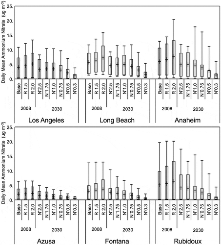
For 2030 with the NO_x emissions the response of the NH₄NO₃ mass concentration to NO_x reductions is much more complicated and nonlinear. The maxima of the NH₄NO₃ mass concentration are not greatly reduced at Central Los Angeles, Long Beach, Anaheim, and Rubidoux until the reductions reach the N’0.50 and N’0.3 cases, while at Azusa and Fontana the response of the maxima is much more linear to NO_x emission reductions. The mean values of the NH₄NO₃ mass concentration at Central Los Angeles, Long Beach, and Anaheim are relatively constant, or they may increase slightly as NO_x emissions are reduced between the N’2.5 and N’1.0 case and the mean values of the NH₄NO₃ mass concentration at all sites decrease as the NO_x emissions are decreased further in the N’1.0, N’0.75, N’0.50, and N’0.30 cases. At Azusa, Fontana, and Rubidoux the mean values of the NH₄NO₃ mass concentration decrease as the NO_x emissions are reduced for all cases.

The upper panel of Figure 10 shows that most of the variation in PM_2.5 with respect to the changes in the NO_x emissions inventory is due to variations in the concentrations of NH₄NO₃(s) for the simulated episodes. Figure 10 is a stack plot of simulated daily-average particulate matter mass concentrations by component at Los Angeles on November 20 for 2008 and 2030 and it is typical of the other sites and days. November 20, 2008, was a day with high measured PM_2.5 mass concentrations. Gas-phase HNO₃ is a necessary precursor of NH₄NO₃(s). The major source of HNO₃ is the reaction of the hydroxyl radical (HO) with NO₂:

(1) $\mathrm{H}\mathrm{O}+\mathrm{N}{\mathrm{O}}_2\to \mathrm{H}\mathrm{N}{\mathrm{O}}_3$(1)

The reaction of HNO₃ with NH₃ is the source of NH₄NO₃, which may exist in solid form depending on atmospheric humidity and temperature (Kim and Seinfeld 1995; Kim, Seinfeld, and Saxena 1993a; 1993b):

(2) $\mathrm{H}\mathrm{N}{\mathrm{O}}_3+\mathrm{N}{\mathrm{H}}_3\to \mathrm{N}{\mathrm{H}}_4\mathrm{N}{\mathrm{O}}_3$(2)

The concentrations of HO are very dependent on NO_x and VOC concentrations. Maximum HO concentrations tend to follow the ridgeline of the O₃ isopleth (Calvert et al. 2015, 478). This is because while NO_x is necessary to produce O₃, HO radicals and HNO₃, its reaction with HO (Reaction 1) terminates free radical chains. Reaction 1 will dominate the gas-phase chemistry if the concentration of NO₂ becomes too high for the ambient VOC concentration, and this will reduce HO concentrations. The competing roles of NO_x as a catalyst for gas-phase atmospheric chemistry and its role as a free radical-chain terminator make HNO₃ production very dependent on NO_x and VOC concentrations. This chemistry is the basis for the O₃ isopleth and the response of HNO₃ production to NO_x and VOC concentrations (Stockwell et al. 2012).

Figure 10. Upper panel presents a stack plot of simulated daily-average particulate matter mass concentrations by component on November 20 for 2008 and 2030 at Los Angeles. The components are secondary organic aerosol (SOA), ammonium nitrate (AmNit), ammonium sulfate (AmSul), unidentified PM_2.5 (unid PM2.5), elemental carbon (EC), primary organic matter (primary OM), and coarse mass. Lower panel presents daily HNO₃ production for differing initial VOC and NO_x concentrations.

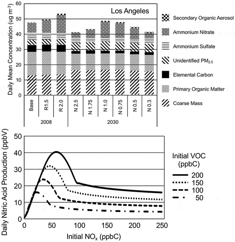
The dependence of HNO₃ on NO_x and VOC concentrations is illustrated by the lower panel of Figure 10. A series of box model simulations were made with a chemical box-model using the Regional Atmospheric Chemical Mechanism, version 2 (RACM2; Goliff, Stockwell, and Lawson 2013). The box-model simulation procedures are described in Fujita et al. (2016). The simulations were made for a range of initial concentrations of NO_x and VOC and they presented the box-model simulations as isopleths. Here the simulated daily production of HNO₃ are plotted in Figure 10 as a function of the initial NO_x for four initial VOC concentrations.

Figure 10 shows that at low NO_x concentrations the production of HNO₃ is limited by the available NO_x. The production of HNO₃ increases almost linearly until it reaches a peak where the production is no longer NO_x limited. The concentration of NO_x where HNO₃ production becomes VOC-limited is determined by the available VOC. Increases in the available NO_x decreases HNO₃ production when the production of HNO₃ becomes VOC limited. This is reflective of the behavior of PM_2.5 seen in the CMAQ simulations shown in Figures 8 and 9 and the upper panel of Figure 10.

Particulate sulfate and secondary organic aerosol

Particulate ammonium sulfate was estimated from the sum of CMAQ simulated Aitken and accumulation mode aerosol sulfate, assuming it had all converted to (NH₄)₂SO₄. The daily average total ammonium sulfate mass concentrations were not strongly affected by the basin-wide VOC or NO_x emissions. Relative to 2008, the daily average total ammonium sulfate mass concentrations were substantially lower at Los Angeles, Long Beach, and Anaheim, a little lower at Azusa and Fontana, and unchanged at Rubidoux for 2030 (Stockwell et al. 2017).

The daily average secondary organic aerosol concentrations are relatively small in our CMAQ simulations, as shown in the upper panel of Figure 10. The simulations show that greater reductions in NO_x emissions lead to higher daily average secondary organic aerosol concentrations (Stockwell et al. 2017). The same relationship holds for SOA produced from both biogenically and anthropogenically emitted VOC. However, there is literature that suggests that SOA simulations might not be accurate (e.g., Murphy et al. 2017).

Evaluation of the response of PM_2.5 concentrations to ammonia emission changes

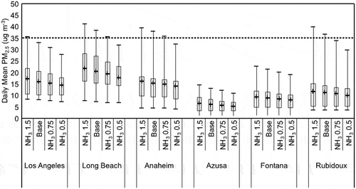
The effects of variations in NH₃ emissions are shown in Figure 11. Daily average PM_2.5 concentrations, NH₄NO₃ mass concentrations, and ammonium sulfate mass concentrations decrease with reductions in NH₃ emissions at all sites. Reductions in these particulate matter concentrations are seen for the first and third quantile, maximum, and mean values at all sites. Figure 11 shows that the PM_2.5 concentrations are below the NAAQS regulations at most sites except for a few extreme events. Most of the reductions in PM_2.5 concentrations are due to the effect of the NH₃ reductions on the formation of NH₄NO₃ and ammonium sulfate (Stockwell et al. 2017). The limitation of PM_2.5 concentrations to NH₃ emissions in the SoCAB is in contrast to the San Joaquin Valley, where NH₄NO₃ formation is more limited by NO_x. However, much of the upwind reactive nitrogen emissions are converted to nitrate prior to entering the San Joaquin Valley (Kleeman, Ying, and Kaduwela 2005). One limitation of our result is that Kelly et al. (2014) have shown there are multiple uncertainties in NH₃ emissions models and inventory. This uncertainty may affect simulations of PM_2.5 for the SoCAB.

Figure 11. Range of predicted daily average PM_2.5 mass concentrations for several adjustments to NH₃ emissions at six monitoring sites in the SoCAB. The box and whisker plots indicate the minimum, first and third quantile, maximum, and mean (+) values during two high PM_2.5 episodes, September 12–15 and November 11–24. The dashed line is the level of the current NAAQS.

Conclusion

Primary PM species, elemental carbon, and organic mass are not affected by changes to the NO_x and VOC emission inventories, but coarse aerosol mass particle concentrations decrease slightly due to reductions in the NO_x emissions inventory. Ammonium nitrate particle concentrations show a strong dependence on the NO_x emissions inventory. The projected 2030 NO_x emission inventory results in lower ammonium nitrate concentrations in 2030 than in 2008. However, the projected 2030 NO_x emission inventory is not the most effective in reducing NH₄NO₃ concentrations of the scenarios that were simulated. Under some conditions, higher NO_x emissions (greater than the projected 2030 inventory) can yield lower maximum PM_2.5 and NH₄NO₃ concentrations in the SoCAB, but greater NO_x reductions may be required to reduce both PM_2.5 and ozone. At Azusa and Fontana, the sites located farthest upwind from the coast, reductions in NO_x emissions decrease NH₄NO₃ for all of the 2030 cases. Ammonium sulfate is not greatly affected by changes in the NO_x and VOC emissions inventory. Secondary organic aerosol increases with increases in the VOC emissions inventory. Decreases in NO_x emissions lead to increases in secondary organic aerosol concentrations. Reductions in NH₃ emissions reduce the formation of PM_2.5 through reductions in the formation of NH₄NO₃ and ammonium sulfate, but additional efforts are needed to improve both NH₃ emission inventories and model treatment of this chemistry. We suggest on the basis of our simulations that a more comprehensive multipollutant plan be developed for improving air quality that focuses on ozone and PM together and that policymakers consider a more optimum strategy involving reductions in NO_x, VOC, and NH₃. This conclusion is supported by the previous study of ozone and PM in the SoCAB by Nguyen and Dabdub (2002).

Acknowledgment

The authors gratefully acknowledge the South Coast Air Quality Management District for providing its CMAQ modeling input and output files for our use.

Additional information

Funding

This project was supported by the Coordinating Research Council (CRC Projects A-101 and A-109), the Truck and Engine Manufacturers Association (EMA), and the NOAA Center for Atmospheric Science—Meteorology (NCAS-M), which is funded by the National Atmospheric Administration/Educational Partnership Program under Cooperative Agreement NA16SEC4810006. Neither the CRC, EMA, NOAA, DRI, UTEP, NASA, their members, nor any person acting on their behalf (1) makes any warranty, express or implied, with respect to the use of any information, apparatus, method, or process disclosed in this report; (2) assumes any liabilities with respect to use of, inability to use, or damages resulting from the use or inability to use, any information, apparatus, method, or process disclosed in this research publication; and (3) this publication presents the independent work and conclusions of its authors and has not been endorsed, accepted, or otherwise approved by any of the funders of the underlying work.

Notes on contributors

Devoun R. Stewart

Devoun R. Stewart is a professor in the Department of Chemistry at Sacramento City College.

Emily Saunders

Emily Saunders is a senior research scientist in the Global Modeling and Assimilation Office at the NASA Goddard Space Flight Center.

Roberto Perea

Roberto Perea is with the Department of Information Technology at UTEP.

Rosa Fitzgerald

Rosa Fitzgerald is a professor in the Physics Department of the University of Texas El Paso (UTEP).

David E. Campbell

David E. Campbell is an associate research scientist in the Division of Atmospheric Sciences at the Desert Research Institute (DRI) (Nevada System of Higher Education).

William R. Stockwell

William R. Stockwell is an affiliated faculty member in the Division of Atmospheric Sciences at DRI and a research professor in the Physics Department at UTEP.

References

- Binkowski, F. S. 1999. Chapter 10. Aerosols in MODELS-3 CMAQ. In Science algorithms of the EPA models-3 Community Multiscale Air Quality (CMAQ) modeling system, eds. Q. W. Byun and J. K. S. Ching. Washington, DC, USA: EPA Report EPA-600/R-89-030, U.S. Environmental Protection Agency.
- Binkowski, F. S., and U. Shankar. 1995. The regional particulate model 1. Model description and preliminary results. J. Geophys. Res. 100:26191–26209. doi:10.1029/95JD02093.
- Brunekreef, B., and S. T. Holgate. 2002. Air pollution and health. The Lancet 360:1233–1242. doi:10.1016/S0140-6736(02)11274-8.
- Byun, D., and K. L. Schere. 2006. Review of the governing equations, computational algorithms, and other components of the Models-3 Community Multiscale Air Quality (CMAQ) modeling system. Appl. Mech. Rev. 59:51–77. doi:10.1115/1.2128636.
- Byun, Q. W., and J. K. S. Ching. 1999. Science Algorithms of the EPA Models-3 Community Multiscale Air Quality (CMAQ) Modeling System. EPA Report EPA-600/R-89-030, U.S. Environmental Protection Agency, Washington, DC, USA.
- Calvert, J. G., J. J. Orlando, W. R. Stockwell, and T. J. Wallington. 2015. The mechanisms of reactions influencing atmospheric ozone. Oxford, UK: Oxford University Press, Oxford.
- Chen, D., Q. Li, J. Stutz, Y. Mao, L. Zhang, O. Pikelnaya, J. Y. Tsai, C. Haman, B. Lefer, B. Rappenglück, S. L. Alvarez, J. A. Neuman, J. Flynn, J. M. Roberts, J. B. Nowak, J. de Gouw, J. Holloway, N. L. Wagner, P. Veres, S. S. Brown, T. B. Ryerson, C. Warneke, and I. B. Pollack. 2013. WRF-Chem simulation of NOx and O3 in the L.A. basin during CalNex-2010. Atmos. Environ. 81:421–432. doi:10.1016/j.atmosenv.2013.08.064.
- Chow, J. C., J. G. Watson, L.-W. A. Chen, M. C. O. Chang, N. F. Robinson, D. Trimble, and S. Kohl. 2007. The IMPROVE_A temperature protocol for thermal/optical carbon analysis: Maintaining consistency with a long-term database. J. Air Waste Manage. Assoc. 57:1014–1023. doi:10.3155/1047-3289.57.9.1014.
- Cohen, A. J., M. Brauer, R. Burnett, H. R. Anderson, J. Frostad, K. Estep, K. Balakrishnan, B. Brunekreef, L. Dandona, R. Dandona, V. Feigin, G. Freedman, B. Hubbell, A. Jobling, H. Kan, L. Knibbs, Y. Liu, R. Martin, L. Morawska, C. A. Pope, H. Shin, K. Straif, G. Shaddick, M. Thomas, R. van Dingenen, A. van Donkelaar, T. Vos, C. J. L. Murray, and M. H. Forouzanfar. 2017. Estimates and 25-year trends of the global burden of disease attributable to ambient air pollution: An analysis of data from the Global Burden of Diseases Study 2015. The Lancet 389:1907–1918. doi:10.1016/S0140-6736(17)30505-6.
- Eder, B., and S. Yu. 2006. A performance evaluation of the 2004 release of Models-3 CMAQ. Atmos. Environ. 40:4811–4824. doi:10.1016/j.atmosenv.2005.08.045.
- Fujita, E. M., D. E. Campbell, W. R. Stockwell, E. Saunders, R. Fitzgerald, and R. Perea. 2016. Projected ozone trends and changes in the ozone-precursor relationship in the South Coast Air Basin in response to varying reductions of precursor emissions. J. Air Waste Manage. Assoc. 66:201–214. doi:10.1080/10962247.2015.1106991.
- Goliff, W. S., W. R. Stockwell, and C. V. Lawson. 2013. The regional atmospheric chemistry mechanism, version 2. Atmos. Environ. 68:174–185. doi:10.1016/j.atmosenv.2012.11.038.
- Grahame, T. J., R. Klemm, and R. B. Schlesinger. 2014. Public health and components of particulate matter: The changing assessment of black carbon. J. Air Waste Manage. Assoc. 64:620–660. doi:10.1080/10962247.2014.912692.
- Kelly, J. T., K. R. Baker, J. B. Nowak, J. G. Murphy, M. Z. Markovic, T. C. VandenBoer, R. A. Ellis, J. A. Neuman, R. J. Weber, J. M. Roberts, P. R. Veres, J. A. de Gouw, M. R. Beaver, S. Newman, and C. Misenis. 2014. Fine-scale simulation of ammonium and nitrate over the South Coast Air Basin and San Joaquin Valley of California during CalNex-2010. J. Geophys. Res. 119:3600–3614.
- Kim, Y. P., and J. H. Seinfeld. 1995. Atmospheric gas–Aerosol equilibrium III. Thermodynamics of crustal elements Ca2+; K+; and Mg2+. Aerosol Sci. Technol. 22:93–110. doi:10.1080/02786829408959730.
- Kim, Y. P., J. H. Seinfeld, and P. Saxena. 1993a. Atmospheric gas–Aerosol equilibrium I. Thermodynamic model. Aerosol Sci. Technol. 19:157–181. doi:10.1080/02786829308959628.
- Kim, Y. P., J. H. Seinfeld, and P. Saxena. 1993b. Atmospheric gas–Aerosol equilibrium II. Analysis of common approximations and activity coefficient calculation methods. Aerosol Sci. Technol. 19:182–198. doi:10.1080/02786829308959629.
- Kleeman, M. J., Q. Ying, and A. Kaduwela. 2005. Control strategies for the reduction of airborne particulate nitrate in California’s San Joaquin Valley. Atmos. Environ. 39:5325–5341. doi:10.1016/j.atmosenv.2005.05.044.
- Makar, P. A., M. D. Moran, Q. Zheng, S. Cousineau, M. Sassi, A. Duhamel, M. Besner, D. Davignon, L.-P. Crevier, and V. S. Bouchet. 2009. Modelling the impacts of ammonia emissions reductions on North American air quality. Atmos. Chem. Phys. 9:7183–7212. doi:10.5194/acp-9-7183-2009.
- Murphy, B. N., M. C. Woody, J. L. Jimenez, A. M. G. Carlton, P. L. Hayes, S. Liu, N. L. Ng, L. M. Russell, A. Setyan, L. Xu, J. Young, R. A. Zaveri, Q. Zhang, and H. O. T. Pye. 2017. Semivolatile POA and parameterized total combustion SOA in CMAQv5.2: Impacts on source strength and partitioning. Atmos. Chem. Phys. 17:11107–11133. doi:10.5194/acp-17-11107-2017.
- Nguyen, K., and D. Dabdub. 2002. NOx and VOC and its effects on the formation of aerosols. Aerosol Sci. Technol. 36:560–572. doi:10.1080/02786820252883801.
- Sicard, P., A. Mangin, P. Hebel, and P. Mallea. 2010. Detection and estimation trends linked to air quality and mortality on French Riviera over the 1990–2005 period. Sci. Total Environ. 408:1943–1950. doi:10.1016/j.scitotenv.2010.01.024.
- South Coast Air Quality Management District. 2013, February. Final 2012 air quality management plan. Diamond Bar, CA: SCAQMD.
- South Coast Air Quality Management District. 2017, March. Final 2016 air quality management plan. Diamond Bar, CA: SCAQMD. https://www.aqmd.gov/home/air-quality/clean-air-plans/air-quality-mgt-plan/final-2016-aqmp.
- Spada, N. J., and N. P. Hyslop. 2018. Comparison of elemental and organic carbon measurements between IMPROVE and CSN before and after method transitions. Atmos. Environ. 178:173–180. doi:10.1016/j.atmosenv.2018.01.043.
- Stewart, D. 2017. Air quality modeling and health and economic assessment of projected ozone and particulate matter response to varying reductions of oxides of nitrogen and volatile organic compound emissions in the south coast air basin. Ph.D. Dissertation, Howard University.
- Stewart, D., E. Saunders, R. A. Perea, R. Fitzgerald, D. E. Campbell, and W. R. Stockwell. 2017. Linking air quality and human health effects models: An application to the Los Angeles Air Basin. Environ. Health Insights 11:1–13. doi:10.1177/1178630217737551.
- Stockwell, W. R., C. V. Lawson, E. Saunders, and W. S. Goliff. 2012. A review of tropospheric atmospheric chemistry and gas-phase chemical mechanisms for air quality modeling. Atmosphere 3:1–32. doi:10.3390/atmos30100012011.
- Stockwell, W. R., R. Fitzgerald, R. Perea, D. E. Campbell, D. Stewart, and E. Saunders. 2017. Air quality modeling of the relationship between projected ozone and pm trends and changes in precursor relationships in the south coast air basin in response to varying reductions of precursor emissions. Final Report for CRC Project A-101, Coordinating Research Council, Atlanta, GA.
- U.S. EPA. 2007. Guidance on the Use of Models and Other Analyses for Demonstrating Attainment of Air Quality Goals for Ozone, PM2.5, and Regional Haze. U.S. Environmental Protection Agency, Research Triangle Park, North Carolina. Accessed August 13, 2018. https://www3.epa.gov/scram001/guidance/guide/final-03-pm-rh-guidance.
- Yu, H., A. Russell, J. Mulholland, T. Odman, Y. Hu, H. H. Chang, and N. Kumar. 2018. Cross-comparison and evaluation of air pollution field estimation methods. Atmos. Environ. 179:49-60.