A novel bagging ensemble approach for predicting summertime ground-level ozone concentration

ABSTRACT

Ozone pollution appears as a major air quality issue, e.g. for the protection of human health and vegetation. Formation of ground level ozone is a complex photochemical phenomenon and involves numerous intricate factors most of which are interrelated with each other. Machine learning techniques can be adopted to predict the ground level ozone. The main objective of the present study is to develop the state-of-the-art ensemble bagging approach to model the summer time ground level ozone in an industrial area comprising a hazardous waste management facility. In this study, the feasibility of using ensemble model with seven meteorological parameters as input variables to predict the surface level O3 concentration. Multilayer perceptron, RTree, REPTree, and Random forest were employed as the base learners. The error measures used for checking the performance of each model includes IoAd, R2, and PEP. The model results were validated against an independent test data set. Bagged random forest predicted the ground level ozone better with higher Nash-Sutcliffe coefficient 0.93. This study scaffolded the current research gap in big data analysis identified with air pollutant prediction.

Implications: The main focus of this paper is to model the summer time ground level O₃ concentration in an Industrial area comprising of hazardous waste management facility. Comparison study was made between the base classifiers and the ensemble classifiers. Most of the conventional models can well predict the average concentrations. In this case the peak concentrations are of importance as it has serious effect on human health and environment. The models developed should also be homoscedastic.

Introduction

In the recent years, ground-level ozone (O₃) has become a serious concern in many countries across the world (Ghorani-Azam, Riahi-Zanjani, and Balali-Mood 2016). Ground-level O₃ is a secondary pollutant, and is formed when the primary pollutants nitrogen oxides (NO_X) and volatile organic compounds (VOCs) react in the presence of sunlight (Liu et al. 2018). NO_X and nonmethane VOCs are considered to be the major precursors of surface-level ozone, and the other precursors include carbon monoxide, methane, and sulfur dioxide. To date, surface O₃ is considered as the most damaging air pollutant in terms of adverse effects on human health, vegetation, crops, and materials in Europe (Anav et al. 2015; Calatayud et al. 2016; Javanmardi et al. 2018; Proietti et al. 2016; Sicard, Serra, and Rossello 2016) and may become worse in the future (Sicard et al. 2017). Since the precursors of O₃ have a long lifetime, varying from few hours to a day, depending on humidity, temperature, and air movement, O₃ acts as a transboundary pollutant (Brankov et al. 2003; Gabusi et al., 2005). O₃ is toxic, as it is a strong oxidant, and its toxicity levels for 95 large communities in United States were studied by Swanson and Chapman (2018). They reported that every 10-ppb increase of O₃ resulted in 0.52% higher risk of non-injury-related daily mortality in the following week. Also, they mentioned that the same level of increase in O₃ might result in 0.64% increase in mortality due to cardiovascular or respiratory diseases. As per the World Health Organization, daily mortality rates can rise by 0.3% for every additional 5 ppb of ozone in the air. Owing to its strong oxidizing power, O₃ can damage the lung tissue (Gorai et al. 2015) and weaken the immune system of human beings. Also, O₃ can cause impairment of rubber goods (Lee, Holland, and Falla 1996) and surface coating of materials (Jellinek 1973). In addition, O₃ causes membrane damage on leaves, especially in plants like bean, tobacco, birch, and so on (Lefohn et al. 2018). Furthermore, surface O₃ is the third most important greenhouse gas in terms of radiative forcing contributing to climate change (Beli 2006).The formation of O₃ is considered to be a complex reaction since the production of O₃ is altered by the influence of solar intensity, meteorological conditions, NO_X and VOC ratio, and type of hydrocarbon (Finlayson-Pitts and Pitts 2000; Jenkin and Clemitshaw 2002). Research work focused on identifying the factors causing O₃ formation and its transport have been reported in literature.

Also, recent studies have reported a statistically strong relationship between peak O₃ levels and meteorological parameters, NO_X, and VOCs (Thi et al. 2017). Modeling of ground-level O₃ has been one of the notable topics in the last decade among the air pollution community. Numerous approaches for predicting ground level O₃ have been reported in the literature (Lu and Wang 2014a). These approaches can be categorized as follows: the traditional statistical approach, the deterministic approach (chemistry transport models), the geo-statistical approach, and machine learning. Traditional statistical approaches include multiple linear regression (Abdul-Wahab, Bakheit, and Al-Alawi 2005), multiple linear regression combined with principal component analysis (Tan, San Lim, and Jafri 2016), and DAUMOD-GRS models (Pineda Rojas, Venegas, and Mazzeo 2016). O₃ concentrations are influenced by chemical emissions, physical processes, and atmospheric conditions (Watson et al. 1998). The multiple linear regression method was widely used because of the convenience of establishing a relationship between O₃ and the variables associated with its behavior, through an explicit equation (Barrero, Grimalt, and Cantón 2006). On the other hand, the nonlinear relationship between O₃ and its contributing factors makes the linear models unfit (Cannon et al. 2011). Multiple linear regression also suffered from the limitation that for obtaining the best fit, it needs the local data of the variables, in relationship with the predicted variable (Awang et al. 2015). Furthermore, the complexity of O₃ formation, combined with the uncertainty in the measurement of parameters involved, makes the modeling process intricate.

In order to handle the complicated chemical reactions involved in the O₃ formation, atmospheric chemical models such as WRF CHEM, WRF CMAQ, and CHIMERE (Boynard et al. 2011; Hoshyaripour et al. 2016) were used for modeling tropospheric O_3. These models were formulated in such a manner that one can understand the impact of air pollutant emissions on the chemical composition of the atmosphere and corresponding consequences on the environment (Gupta and Mohan 2015). With finer grid resolution and with improvement in temporal and spatial resolution of emission inventory, an efficient model can be developed with much less uncertainty (Karlický et al. 2017). On the contrary, the key limitations of these models include the requirements of higher computational resources and good knowledge about the atmospheric processes and source of pollution (Tong, Leung, and Liu 2011). Also, these models tend to underestimate the magnitude of fluctuations on shorter time scales and the possibility of overprediction during the periods of extensive cloud cover (Pal et al. 2014).

Although the O₃ formation and the dispersion of the precursors in the troposphere are intricate, researchers have made significant efforts to simplify this complex behavior and to understand the characteristics of their distribution over time. Tropospheric O₃ is a transboundary problem and it is economically unviable to establish stations in each place of interest, especially in rural areas (Adame and Sole 2013). In such cases, geo-statistical models are of great value. Land use regression and ordinary kriging comprise the most commonly used geo-statistical approach for O₃ prediction (Jerrett et al. 2004). Each geo-statistical model has inherent uncertainty due to the complexity of the atmospheric environment (Adam-Poupart et al. 2014). O₃ maps developed using geo-statistical methods can influence decisions concerning air-quality policy, which, in turn, can affect the attitudes and behaviors of the general public.

With the development of data mining tools, machine learning techniques such as multilayer perceptron (Mishra and Goyal 2016), support vector machine (Gong and Ordieres-Meré 2016), and the ensemble approach (bagging) (Al Abri et al. 2015) have gained much interest, For example, neural networks proved to be a strong nonlinear estimator, except with the limitation of overfitting (Singh, Gupta, and Rai 2013).

In recent years, researchers have focused on advanced models like ensemble models, which showed better performance than standard single machine learning classifiers (Gong and Ordieres-Meré 2016). Ensemble classifiers proved to perform well when compared to single base classifiers in sectors like banking and medical applications and in industrial applications (Erdal and Karahanoğlu 2016). Three types of ensemble methods are bagging, boosting, and stacked generalization. Bagging (boot strap aggregating) technique was developed by Breiman. Bagging decreases the residual error between the observed and predicted values by creating bootstrapped replica data sets (Friedman 2002). Cannon et al. (2011) adopted ensemble neural network approach for predicting the summer-season O₃ levels. Ensemble neural network models showed a 7% increase in the variance compared to multiple linear regression models. Singh, Gupta, and Rai (2013) used the ensemble trees to predict the air quality, utilizing meteorological parameters as estimators. The performance was checked in terms of classification as well as regression. They found that both bagging and boosting trees performed better than the single support vector machine (SVM) classifier. These studies have the limitation that bagging was employed with REPTree, which is the default classifier associated with bagging.

In this paper, the relative advantages of ensemble bagging classifiers over base classifiers such as multilayer perceptron, RTree, REPTree, and random forest for predicting summertime ground-level O₃ prediction are analyzed and presented. A comparative study was carried out to assess the performance of machine learning techniques using the WEKA toolkit (WEKA 3.8.2). The main objectives of the present study are (i) to develop ensemble bagging model to accurately predict ground-level O₃, with emphasis on peak levels/high concentration, and (ii) to evaluate the capabilities of each modeling technique. A comparative analysis assessing the performance of ensemble bagging classifiers and single classifier in predicting O₃ concentration is also presented in this paper.

Materials and methods

Description of the study area and data set

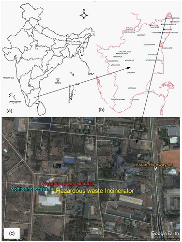
An industrial site at Gummidipoondi town with geographical position of 13.4069º N and 80.1103° E and located 45 km north of Chennai city, Tamil Nadu, India, was chosen for the ozone measurements. The industrial complex in which the study area is located comprises steel, chemicals, auto ancillary, auto components, and plastic industries. In particular, the monitoring location is nearby a hazardous waste management facility, which includes an incinerator and a landfill. In addition, Asian Highway 45 (AH 45) is located at a distance of 500 m from the study location. The study area is illustrated in Figure 1. The hazardous waste landfill facility has a storage facility where hazardous wastes such as solvents, flammables, explosive items, pharmaceutical wastes, and others were stored. In addition to the VOCs emanating from the landfill, these stored hazardous wastes acted as a key source of VOCs. NO_X is produced mainly from the vehicles moving inside the industrial area and from those plying the AH 45 road. This would result in large concentrations of O₃ in the study area.

Figure 1. (a) Map of India. (b) Map of Tamil Nadu. (c) Map showing the study area at Gummidipoondi (domain size: (length × height: 1.5 km × 2.4 km). (a), (b) Image source: maps of India. (c) Image source: Google Earth Pro.

An O₃ 42 M analyzer was used to measure the ozone concentration at the site. The O₃ analyzer was installed in an existing building at the site. The inlet tube of the O₃ analyzer was open to the atmosphere outside the building, at a height of 3 m. NO_X measurements were done using a 32M NO_X analyzer. This instrument was kept beside the O₃ analyzer. The NO_X analyzer works on the principle of chemiluminiscence. The gas measurements were recorded every 15 min to depict the O₃ and NO_X variations. Meteorological parameters were measured using a Spectrum Watchdog 2000 series weather station, model 2900ET.

Continuous measurements of all the parameters, namely, O₃, NO, NO₂, and meteorological parameters, were carried out during the period between January 2016 and December 2016 except during the maintenance of the analyzers. Three months of data between March 2016 and May 2016 (summer season) was utilized for the present modeling. The formation of O₃ is through photochemical reaction, the solar radiation facilitates the formation of photochemical oxidants. The concentration of O₃ decreases when the photochemical reaction ceases and when the concentrations of precursors are lower. The peak concentrations of O₃ occur during the daytime, and it can pose health risk in the workers and other people in the surrounding areas. Hence, in the present study, the O₃ concentrations measured between 07:00 a.m. and 06:00 p.m. are used for modeling. In the study period, the final data set with complete O₃ and meteorological data covers 1012 hourly observations. Based on the earlier studies (Gao, Yin, and Ning 2018), seven meteorological parameters, namely, solar irradiance, relative humidity, temperature, rainfall, wind speed, and wind direction (two components), were selected as the predictor variables. Since industrial and vehicular emissions are the major sources of O₃ in the study area, the data obtained on weekdays (high industrial emissions) and weekends (high vehicular emissions) are not separated.

Ensemble method

Ensemble methods are meta-algorithms that combine several machine learning techniques into one predictive model to decrease variance and bias and to improve predictions (Xiao et al. 2018). While the computational times of decision trees are lower, the prediction accuracy is moderate and a multilayer perceptron (Jiang et al. 2010) handles the nonlinear chaotic system with high accuracy. However, these models fail to predict extreme concentrations and large local-scale variations of concentrations (Wang and Song 2018). In addition, single classifiers suffer from any/all of the three fundamental limitations, namely, statistical, computational, and representational. Ensemble methods have the advantage of reducing these key shortcomings of standard learning algorithms (Dietterich 2000). Ensembles are well-established methods for obtaining accurate classifiers, by combining the less accurate ones. The ensemble approach reduces the bias by effectively using the training dataset. Also, it lowers the variance by combining the outputs multiple times from the same learning method.

Bagging

Bagging takes a bootstrap sample of data and trains a classifier on each sample. In the present study, bagging with average aggregation is implemented in WEKA. MLP and decision trees are commonly used as base predictors in ensemble models and enhanced using bagging techniques.

For a regression problem, bagging works as follows (Hacer et al. 2015):

A training set D consists of data {(X_i, Y_i)_{i=1, 2…, n}} where X_i is a realization of a multidimensional predictor variable and Y_i is a realization of a real-valued variable. A predictor $\left(Y|X=x\right)=f\left(x\right)$ is denoted by

(1) $C_n\left(x\right)=h_n\left(D_1,\dots D_n\right)\left(x\right)$(1)

Bagging is explained as follows.

Step 1: Creating a bootstrapped sample:

(2) $D_i^{\ast }=\left(Y_i^{\ast },X_i^{\ast }\right)$(2)

according to the empirical distribution of the pairs D_i = (X_i,Y_i) where (i = 1,2,…,n).

(3) $C_n^{\ast }\left(x\right)=h_n\left(D_1^{\ast },\dots ,D_n^{\ast }\right)\left(x\right)$(3)

Step 2: Assessing the bootstrapped predictor by the plug-in-principle, where C_n(x) = h_n(D₁…,D_n)(x).

Finally, the bagged predictor is

(4) $C_{n:B}\left(x\right)=E\left|D_n^{\ast }\left(x\right)\right|$(4)

The procedure for the model development of ensemble bagging trees is shown in Figure 2.

Figure 2. Processes involved in model development of ensemble bagging tree.

Evaluation of model performance

Willmott’s index of agreement (IoAd), squared differences (given by eq 5), is used for analyzing the performance of the model in predicting the peak values. It is calculated as the ratio between the mean squared error and the potential error (Willmott 1981). This test parameter is highly sensitive to peak observations. Also, in the present study, the Nash–Sutcliffe coefficient, R², given by eq 6, is used to evaluate the model. R² is calculated since it is sensitive to the differences in observed and modeled means and variances (Nash and Sutcliffe 1970). The R² value is also highly sensitive to peak concentration values and is insensitive to low concentration values (Dawson, Adams, and Pandis 2007). A high IoAd and a high R² value indicate good model performance, and vice versa.

Percent error in peak (PEP), given by eq 7, is also calculated to analyze the performance of the model in predicting peak values (Green and Stephenson 1986). This metric was used with utmost care since the data consists of multiple peaks and this measure does not attempt to represent the temporal relationship existing in the data. As per Indian national ambient air quality standards, the threshold limit value for hourly average of ambient O₃ concentration is 180 μg/m³. In the present study, the hourly average O₃ concentrations greater than 180 μg/m³ are selected as peak values. The best fitting ensemble model developed in this paper will be evaluated using PEP values. The percentage error range considered in this study is 5, 10, 15, and 20.

(5) $IoAd=1-\left[\frac{{\sum }_{j=1}^n{(P_{ij}-O_j)}^2}{{\sum }_{j=1}^n{\left(\left|P_{ij}-{\mu }_o\right|+\left|O_j-{\mu }_o\right|\right)}^2}\right]$(5)

(6) $R^2=1-\frac{{\sum }_{i=1}^n{\left(O_j-P_{ij}\right)}^2}{{\sum }_{i=1}^n{\left(O_j-{\mu }_o\right)}^2}$(6)

(7) $PEP=\frac{max\left(O_j\right)-\mathrm{m}\mathrm{a}\mathrm{x}\left(P_{ij}\right)}{\mathrm{m}\mathrm{a}\mathrm{x}\left(O_j\right)}\ast 100$(7)

Model building

In the present study, prediction of surface ozone concentrations was carried out using data mining algorithms. The process was instigated using machine learning open-source software WEKA 3.8.2. Two types of data analysis exist: classification and prediction. Models are built based on the information obtained from important attribute classes. Meta-Bagging classifier is used for the present study. Both explorer and experimenter environments in WEKA were used for the data analysis. Instance-based machine learning classifiers such as decision stump, Rtree and reduced error pruning tree, random forest, MLP, and SMOreg were employed as the base learner. To reduce the impact of the variability of the training set, the experiments were repeated 100 times. Each time, all algorithms were trained on the same portion of the training data and evaluated on the same test data. Initially, runs were performed using the default parameters and the results obtained using default parameters were optimal. Hence, selection of optimal parameters becomes essential for the better prediction of O₃ in both base learner and bagging.

The schematic of the methodology adopted in the present study is shown in Figure 3. By simultaneously tuning the parameters in bagging as well as the base learner, the improvement in R² value was calculated. The R² value was used to check the goodness of the fit and the relationship present in the data. Also, this error measure outlines the degree of descriptiveness of the regression model. To check the statistical significance among the prediction models, a Wilcoxon signed-rank test (two-tailed test at 95% confidence level) was carried out. Note that the Wilcoxon signed rank test was not influenced by the outlier data points.

Figure 3. Schematic diagram showing the proposed modeling methodology.

Inputs selection

Nine predictor variables, including seven meteorological variables and two photochemical parameters, were considered for each data set. Initially, the model was developed using all the nine predictor variables and was used as a benchmarking model. Since, the photochemical parameters NO and NO₂ are difficult to predict (unless using some dynamical models enabled with chemistry), only the seven meteorological parameters were used for developing the model. The model performance was evaluated by using the two metrics IoAd and R².

Data preprocessing

Data preprocessing is an essential stage in obtaining the final data set, which can be used for further data mining. In the data set, there were missing values and outliers, which were recorded during the malfunctioning of analyzers, during high temperatures, and with clogging of filter paper. In order to remove these outliers, data preprocessing techniques such as “interquartile range for attributes” and “remove with values for instances” were adopted. Wind direction is considered as one of the attributes for predicting the O₃ concentration. It was measured with reference to 360° on the compass (true north), in a clockwise direction. The data possess 0° and 360°, which will be considered as different values by the algorithm. To avoid such an error, wind speed and wind direction were combined together. Sine and cosine functions of the wind direction were calculated and replaced with wind direction. Attribute selection was done using filters such as CfssubsetEval (Best first and Greedystepwise), principal components, and ReleifFattributeEval. However, there were no improvements in the prediction accuracy by using such filters. Rather, the values of error measures deteriorated through the application of such filters, as this resulted in the loss of input information.

Cross-validation

The main objective of cross-validation is to determine how well the model has predicted the target values. A “k-fold” cross validation technique is used in this study, which can help in avoiding the problem of overfitting. Ten-fold cross-validation was used to create the models. This involves splitting the data set into 10 equal subsets and using nine subsets as training data and one as test data. The procedure was iterated 10 times so that every subset was utilized as test data once. The final model was then the average of the 10 iterations. The prediction error is calculated as the difference between the observed and predicted values. Model accuracy relies on the factors such as unbiased predictions, closeness of predicted values to target values, and accurate standard errors.

Air mass back trajectory—HYSPLIT

Air trajectory models are mainly used to analyze the dynamical processes occurring in the atmosphere. In particular, for understanding the long-range transport of pollutants, back trajectories are used. These back trajectories are estimated using the Hybrid Single Particle Lagrangian Integrated Trajectory (HYSPLIT). In the present study, the HYSPLIT model (version 6), which is an improved version, was used. Seven days of back trajectories arriving at the surface were computed. Back-trajectory analysis ascertains the area of origin of air masses and determines the source–receptor relationships. The only drawback of this model is its inability to indicate the origin of a specific pollutant.

Results and discussion

Model development

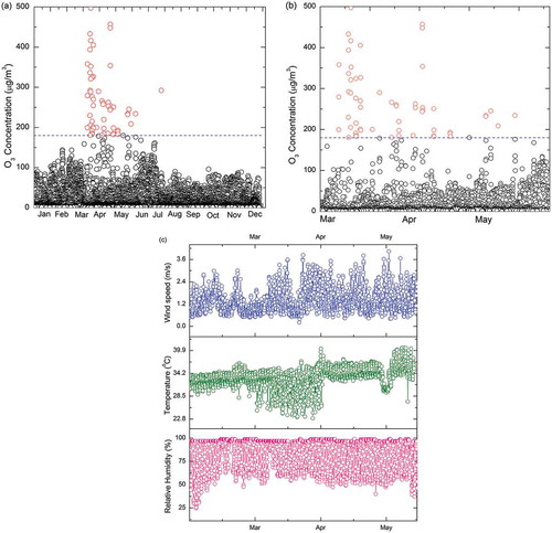
In total, 8278 hourly instances were recorded during the entire study period. The summer data set comprising 1012 daytime instances recorded between March 2016 and May 2016 was used for the model development. By random selection, 847 instances (daytime, 07:00 a.m. to 06:00 p.m.) were used in training and validation process and 165 instances (daytime) were used for the testing process. The time-series plot of the O₃ variation for the entire study period is shown in Figure 4a. Figure 4b shows the time series of the O₃ concentrations during the summer season. The hourly variations of temperature, relative humidity, and wind speed during the summer season are shown in Figure 4c. The statistical summary of the data set is given in Table 1. Trials were conducted to evaluate the performance and the suitability of different classifiers for the data set. The selected classifiers were fine tuned by changing the parameters and by checking with each of the performance measures.

Table 1. Statistics summary of the attributes for the prediction of ground-level O₃ concentration during the study period.

	Statistics summary (training set) (847 Instances)				Statistics summary (test set) (165 Instances)
Attribute	Minimum	Maximum	Mean	Std. dev.	Minimum	Maximum	Mean	Std. dev.
O3 (µg/m^3)	15.44	497.232	61.64	61.35	20.98	398.928	61.55	46.87
Relative humidity (%)	24.53	99.07	82.128	17.78	21.5	99.1	77.7	15.8
Temperature (°C)	28.86	40.59	33.019	2.60	32.58	40.3	30.2	2.8
Wind speed (mph)	0.21	4.04	1.36	0.621	0.15	4.5	1.9	0.7
Wind direction (degrees)	0	358	142.16	101.32	0	355	169	83
Solar radiation (W/m^2)	50.48	933.5	296.69	265.5	65.71	924.9	273.83	272.6

Figure 4. (a) Time-series plot of O₃ across the entire study period (January 2016–December 2016). The dashed line indicates the threshold limit value of hourly ambient O₃ concentration (180 μg/m³). Observed O₃ concentration greater than 180 μg/m³ marked using red circles are considered as peak values. (b) Time-series plot of O₃ during summer season (March 2016–May 2016). The interpretations of the dashed line and red circles are the same as in (a). (c) Hourly variation of relative humidity, temperature, and wind speed (March 2016–May 2016).

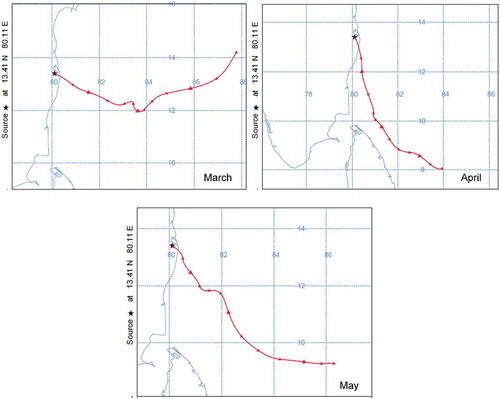
Back-trajectory analysis of air mass (shown in Figure 5) was carried out using HYSPLIT. Figure 5 shows that during the summer months, the air mass had a marine origin and was relatively clean. Hence, the high concentration of O₃ observed during the summer months was mainly due to background O₃, the photochemical reaction of the precursors present in the site, and the local transportation.

Figure 5. Seven days air mass back trajectory using HYSPLIT reaching the monitoring location (March 2016–May 2016).

Prediction of O₃ using bagging ensemble method

The building of an ensemble consists of two steps, namely, the creation of individual ensemble members and the appropriate consolidation of output from the individual ensemble learners. In the present study, an ensemble learning approach and, in particular, bootstrap aggregating (bagging) were adopted to predict the surface O₃ concentration. The bagging algorithm is predominantly used as an ensemble learning method. The parameters associated with the bagging technique are the number of iterations and the bag size percent. In the present study, the numbers of iterations were chosen as 100, 200, 300, 400, and 500 and the sizes of bag as 60%, 70%, 80%, 90%, and 100%. By default, the number of iterations is 10 and the bag size is 100%. For all the models, the number of seed was taken as 1. This resulted in a total of 25 bagging models for each base classifier. The performances of the optimized models were analyzed using IoAd and R² and are given in Table 2. It can also be observed from Table 2 that even after excluding the photochemical parameters NO and NO₂, there is no improvement in the model output. Also, it is very difficult to predict the values of NO and NO₂ using models with higher accuracy. Hence the final ensemble model had only seven meteorological parameters as the predictor variables. Optimal parameters for bagging were selected such that IoAd and R² values were close to unity for those selected parameters.

Table 2. Performance of the bagging classifier for predicting ground-level O₃ concentration.

	Without NOX		With NOX
	IoAd	R^2	IoAd	R^2
MLP	0.73	0.40	0.71	0.38
Bagged MLP	0.64	0.67	0.64	0.57
RTree	0.75	0.57	0.76	0.55
Bagged RTree	0.78	0.69	0.75	0.61
REPTree	0.62	0.69	0.60	0.62
Bagged REPTree	0.69	0.71	0.65	0.68
Random forest	0.82	0.70	0.80	0.69
Bagged random forest	0.96	0.93	0.93	0.86

Model performance

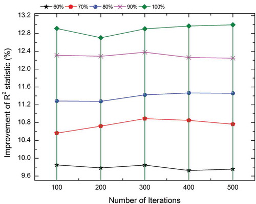
In case of random forest, the improvement in R² values for ensemble model is shown in Figure 6. The plots showing the improvements in R² values for other models are given in the supplementary section (Figures S1a, S1b, and S1c). By simultaneously tuning the parameters in bagging as well as the base learner, the improvement in R² values for MLP, RTree, REPTree, and random forest is 21.5%, 30.6%, 7.4%, and 13.1%, respectively.

Figure 6. Improvement of R² statistic for various iteration and cluster size in case of bagged random forest.

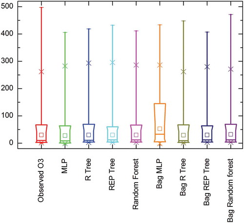
The distributions of the observed and the predicted concentrations are shown as a box plot in Figure 7. In Figure 7, the square box indicates the median, the horizontal lines at the top and bottom indicate the maximum and minimum value, and “x” depicts the 1st and 99th percentiles. The skewness of the actual and the predicted data was analyzed for all the methods and the data set was found to be positively skewed. From Figure 7, it can be observed that, considering the distribution of actual data, the performance of the bagged random forest is better than the other models. The results of the Wilcoxon signed-rank test are given in Table 3. The test results given in Table 3 indicate that the RTree, REPTree, and bagged RTree models follow a similar trend.

Table 3. Wilcoxon signed rank test for base classifiers and bagged classifiers.

	MLP	Rtree	REPTree	Random forest	B-MLP	B-Rtree	B-REPTree	B-Random forest
MLP	—
Rtree	−13.036*	—
REPTree	−11.5*	−7.967	—
Random forest	−10.396*	−9.394*	−2.946*	—
B-MLP	−12.141*	−2.553*	−8.498	−11.095	—
B-Rtree	−10.731*	−7.071*	−0.073	−2.552*	−8.173	—
B-REPTree	−10.596*	−7.397*	−1.389	−1.489	−11.67	0.99*	—
B-Random forest	−9.579*	−8.994*	−4.038*	−4.519*	−12.662	−4.04*	−3.319*	—

Note. *Significant at 0.05 level.

Figure 7. Box plot representation of observed vs. predicted concentration for single base models and bagged ensemble models.

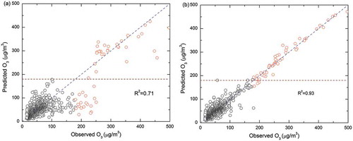
The scatter plots of the observed and the predicted O₃ concentrations corresponding to random forest and bagged random forest models are shown in Figures 8a and 8b, respectively. (Figures S2a, S2b, S2c, S2d, S2e, and S2f corresponding to other classifiers are included in the supplementary section). From Figures 8a and 8b, it can be observed that the bagged random forest model performed better compared to other models. Figures 8a and 8b confirm that the predicted peak value points remained fairly constant between the base classifiers except for the random forest classifier. A big shift in values close to the 45° line can be observed in the case of bagged REPTree and bagged random forest classifiers, but the majority of the peak values remain unchanged in ensemble MLP and RTree classifiers. Also, the variance around the regression line is the same for all the data points in the case of the bagged random forest. Hence the model is homoscedastic in the entire range of data. When compared with the other models, the ensemble random forest performed better with an R² value of 0.95. The other developed models performed well only in a specific range of the data. Thus, the models other than the bagged random forest are heteroscedastic in nature.

Figure 8. Scatter plots of observed vs. predicted ozone for (a) random forest and (b) bagged random forest. The interpretations of the dashed line and red circles are same as in Figure 4a.

The ensemble random forest model produced marginally better performance compared to the other classifiers across the entire data set. Also, the prediction of peak O₃ concentration (Table 4) by the ensemble random forest was much better compared to the other classifiers. The performance of the models for predicting peak concentrations was further confirmed by determining the PEP values (shown in Table 4). There were in total 49 observations with O₃ concentration values greater than 180 µg/m³, out of which 42 peaks were predicted with less than 10% error by the bagged random forest model. This shows the superiority of the bagged random forest over the other models in predicting the O₃ concentration. Further, the bagged random forest predicted all the peaks with less than 20% PEP value.

Table 4. Number of peaks (values >180 μg/m³) having PEP (%) less than the specified range.

	Single classifiers					Ensemble classifiers
	<1%	<5%	<10%	<15%	<20%	<1%	<5%	<10%	<15%	<20%
MLP	0	5	5	4	0	0	9	7	3	2
RTree	4	8	5	6	4	2	8	5	6	4
REPTree	1	10	9	3	0	3	6	7	6	4
Random forest	1	8	10	3	4	10	20	12	5	2

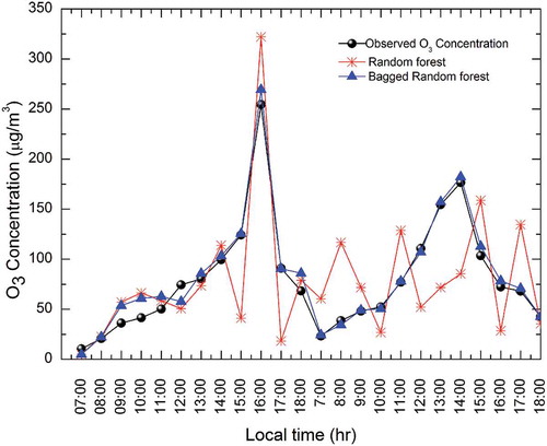
To check the performance of the bagged random forest classifier, an independent data set, which was not included in the training phase, was used. Initially, the test data set was subjected to preprocessing techniques. The prediction of ground-level O₃ by ensemble models is shown in Figure 9. It is evident from Table 5 that the bagged random forest model predicted O₃ concentration better with higher IoAd and R² values. Similar results were reported by Erdal and Karahanoğlu (2016) and Nawahda (2016). From Figure 9, it is evident that the numbers of underpredictions and overpredictions are very low. Also, the peak values, which are the key focus of this study, are predicted well within 5% error range by using the bagged random forest. Hence, the bagged random forest model proved to be an effective and reliable method for predicting the ground-level O₃ concentration. Noted that the execution of these models is subject to the data set that they are applied to.

Table 5. Performance of the Bagging classifier for predicting ground-level O₃ concentration using a test data set.

	IoAd	R^2
MLP	0.68	0.35
Bagged MLP	0.60	0.61
RTree	0.69	0.52
Bagged RTree	0.75	0.60
REPTree	0.70	0.71
Bagged REPTree	0.59	0.65
Random forest	0.78	0.63
Bagged random forest	0.89	0.86

Figure 9. Prediction of hourly O₃ concentration using random forest and bagged random forest for an independent test set (April 10, 2016, and March 28, 2016).

Discussion

The main objective of the present study is to predict the surface-level O₃ concentrations with greater accuracy. O₃ data observed during the summer season were used for the present study. The summer-season data set was chosen since peak O₃ concentrations occurred during the summer season and also large variance in the data set occurred during the summer season. Daytime concentrations include the concentrations recorded between 07:00 a.m. and 06:00 p.m. local time, and the remaining concentrations were included in the nighttime. Low concentrations of O₃ were noticed during the rainy hours. This may be due to the dilution or wash-down of precursor pollutants. Most of the models developed so far for predicting the surface level O₃ have the lacuna that they work well either for the high concentrations or for the low concentrations. In the case of the CMAQ model, researchers have reported that the model predicted well the average concentration, whereas extreme values were either underpredicted or overpredicted (Astitha et al. 2017).

As far as machine learning techniques are concerned, researchers used techniques such as the artificial neural network, support vector machine, random forest, and others for the prediction of ground-level O₃. The major limitations of the artificial neural network were overfitting (Lu and Wang 2014b) and problems in peak value prediction (Mishra and Goyal 2016). The support vector machine generally suffered from a class imbalance problem. Also, the O₃ measurements tend to have a lot of noise and the noises disrupted the training data for building the model. In such cases, bagging helped to reduce the noises present in the data. Bagging trains a large number of strong learners in parallel and finally merges the output of all the strong learners together to smooth out their predictions. Due to the preceding procedure, it also endeavors to avoid the problem of overfitting linked with classifiers such as MLP. The bagged random forest performed well for the entire range of data with an R² value of 0.95, and also the model developed was homoscedastic in nature; 61% of the peak values observed during the study period were predicted with less than 5% PEP measure. The bagged random forest also produced the highest value of IoAd of 0.96 and R² of 0.93.

Conclusion

The objective of the present study is to accurately predict the summertime ground-level O₃ concentration in an industrial area in Chennai, Tamil Nadu, India. The data set included hourly averages of O₃, and meteorological parameters such as relative humidity, temperature, solar irradiance, rainfall, wind speed, and wind direction. Single base classifiers and ensemble classifiers were employed for the prediction of O₃ concentration observed during the summer season. The ensemble classifiers, namely, bagged MLP, bagged RTree, bagged REP tree, and bagged random forest, yielded better results than the respective base classifiers. The improvement in R² values for ensemble models of MLP, RTree, REPTree, and random forest were 21.5%, 30.6%, 7.4%, and 13.1%, respectively. The overall performance of the bagged random forest model was better than the ensemble MLP, RTree, and REPTree models. Also, when compared to other models, the bagged random forest was better in predicting the peak O₃ concentrations. The bagged random forest model developed in this paper was also found to be homoscedastic and parsimonious. Compared to the traditional methods such as MLP and SMOreg, the bagged random forest model gave higher IoAd and R² values of 0.96 and 0.93, respectively. These ensemble models can be used as valuable tools while framing ozone control strategies.

Acknowledgment

The authors gratefully acknowledge the NOAA Air Resources Laboratory (ARL) for granting permission to use its HYSPLIT transport and dispersion model and/or the READY website (http://www.arl.noaa.gov/ready.html) used in this publication. The authors thank the anonymous reviewers for their useful suggestions, which helped in improving the quality of the paper.

Supplementary data

Supplementary data for this paper can be accessed on the publisher’s website.

Additional information

Funding

The authors thank the China Section of the Air & Waste Management Association for the generous scholarship they received to cover the cost of page charges and make the publication of this paper possible. This work was supported by the China Section of the Air & Waste Management Association (jawma28).

Notes on contributors

Sankaralingam Mohan

Sankaralingam Mohan is a professor in the Department of Civil Engineering, Environmental and Water Resources Engineering Laboratory, Indian Institute of Technology Madras, Chennai, India.

Packiam Saranya

Packiam Saranya is a Ph.D. scholar in the Department of Civil Engineering, Environmental and Water Resources Engineering Laboratory, Indian Institute of Technology Madras, Chennai, India.

References

- Abdul-Wahab, S. A., C. S. Bakheit, and S. M. Al-Alawi. 2005. Principal component and multiple regression analysis in modelling of ground-level ozone and factors affecting its concentrations. Environ. Model. Softw. 20:1263–1271. doi:10.1016/j.envsoft.2004.09.001.
- Adame, J. A., and J. G. Sole. 2013. Surface ozone variations at a rural area in the northeast of the Iberian Peninsula. Atmos. Pollut. Res. 4:130–141. doi:10.5094/APR.2013.013.
- Adam-Poupart, A., A. Brand, M. Fournier, M. Jerrett, and A. Smargiassi. 2014. Spatiotemporal modeling of ozone levels in quebec (canada): a comparison of kriging, land-use regression (lur), and combined bayesian maximum entropy-lur approaches. Environ. Health Perspect. 122:970–976. doi: 10.1289/ehp.1306566.
- Al Abri, E. S., E. A. Edirisinghe, A. Nawadha, and U. Kingdom. 2015. Modelling ground-level ozone concentration using ensemble learning algorithms. Int. Conf. Data Min. (DMIN). Steer. Comm. World Congr. Comput. Sci. Comput. Eng. Appl. Comput 148–154.
- Anav, A., A. De Marco, C. Proietti, A. Alessandri, A. Dell’Aquila, I. Cionni, P. Friedlingstein, D. Khvorostyanov, L. Menut, E. Paoletti, P. Sicard, S. Sitch, and M. Vitale. 2015. Comparing concentration-based (aot40) and stomatal uptake (pody) metrics for ozone risk assessment to european forests. Glob. Chang. Biol. 22:1608–1627. doi: 10.1111/gcb.13138.
- Astitha, M., H. Luo, S. T. Rao, C. Hogrefe, R. Mathur, and N. Kumar. 2017. Dynamic evaluation of two decades of WRF-CMAQ ozone simulations over the contiguous United States. Atmos. Environ. 164:102–116. doi:10.1016/j.atmosenv.2017.05.020.
- Awang, N. R., N. A. Ramli, A. S. Yahaya, and M. Elbayoumi. 2015. Multivariate methods to predict ground level ozone during daytime, nighttime, and critical conversion time in urban areas. Atmos. Pollut. Res. 6:726–734. doi:10.5094/APR.2015.081.
- Barrero, M. A., J. O. Grimalt, and L. Cantón. 2006. Prediction of daily ozone concentration maxima in the urban atmosphere. Chemom. Intell. Lab. Syst. 80:67–76. doi:10.1016/j.chemolab.2005.07.003.
- Beli, D. S. 2006. Global warming and greenhouse gases. Physics, chemistry and Technology, Facta Universitatis, 4, 45–55.
- Boynard, A., M. Beekmann, G. Foret, A. Ung, S. Szopa, C. Schmechtig, and A. Coman. 2011. An ensemble assessment of regional ozone model uncertainty with an explicit error representation. Atmos. Environ. 45:784–793. doi:10.1016/j.atmosenv.2010.08.006.
- Brankov, E., R. F. Henry, K. L. Civerolo, W. Hao, S. T. Rao, P. K. Misra, R. Bloxam, and N. Reid. 2003. Assessing the effects of transboundary ozone pollution between Ontario, Canada and New York, USA. Environ. Pollut. 123:403–411. doi:10.1016/S0269-7491(03)00017-4.
- Calatayud, V., Diéguez, J.J., Sicard, P., Schaub, M., De Marco, A. Testing approaches for calculating stomatal ozone fluxes from passive samplers. Sci. Total Environ. 572:56–67. doi: 10.1016/j.scitotenv.2016.07.155.
- Cannon, A. J., E. R. Lord. 2011. Forecasting summertime surface-level ozone concentrations in the lower fraser valley of British Columbia: An ensemble neural network approach. J. Air Waste Manag. Assoc. 50: 322–339.. doi:10.1080/10473289.2000.10464024.
- Dawson, J. P., P. J. Adams, and S. N. Pandis. 2007. Sensitivity of ozone to summertime climate in the eastern USA: A modeling case study. Atmos. Environ. 41:1494–1511. doi:10.1016/j.atmosenv.2006.10.033.
- Dietterich, T. G. 2000. Ensemble methods in machine learning. Mult. Classif. Syst. 1857:1–15. doi:10.1007/3-540-45014-9.
- Erdal, H., and İ. Karahanoğlu. 2016. Bagging ensemble models for bank profitability: An emprical research on Turkish development and investment banks. Appl. Soft Comput. J. 49:861–867. doi:10.1016/j.asoc.2016.09.010.
- Finlayson-pitts, B.J., and J.N. Pitts, 2000. Chemistry of the Upper and Lower Atmosphere. Theory, experiments, and applications, in: Academic Press. p. 969. doi: 10.1016/B978-0-12-257060-5.50027-7
- Friedman, J. H. 2002. Stochastic gradient boosting. Comput. Stat. Data Anal. 38:367–378. doi:10.1016/S0167-9473(01)00065-2.
- Gabusi, V., E. Pisoni, and M. Volta. 2005. Transboundary pollution and local emission impact in tropospheric ozone accumulation processes: Control strategy modelling assessment. Proc. 44th IEEE Conf. Decis. Control 7404–7409. doi:10.1109/CDC.2005.1583356.
- Gao, M., L. Yin, and J. Ning. 2018. Artificial neural network model for ozone concentration estimation and Monte Carlo analysis. Atmos. Environ. 184:129–139. doi:10.1016/j.atmosenv.2018.03.027.
- Ghorani-Azam, A., B. Riahi-Zanjani, and M. Balali-Mood. 2016. Effects of air pollution on human health and practical measures for prevention in Iran. J. Res. Med. Sci. 21:65. doi:10.4103/1735-1995.189646.
- Gong, B., and J. Ordieres-Meré. 2016. Prediction of daily maximum ozone threshold exceedances by preprocessing and ensemble artificial intelligence techniques: Case study of Hong Kong. Environ. Model. Softw. 84:290–303. doi:10.1016/j.envsoft.2016.06.020.
- Gorai, A. K., F. Tuluri, P. B. Tchounwou, and S. Ambinakudige. 2015. Influence of local meteorology and NO(2) conditions on ground-level ozone concentrations in the eastern part of Texas, USA. Air Qual. Atmos. Health 8:81–96. doi:10.1007/s11869-014-0276-5.
- Green, I. R. A., and D. Stephenson. 1986. Criteria for comparison of single event models. Hydrol. Sci. J. 31:395–411. doi:10.1080/02626668609491056.
- Gupta, M., and M. Mohan. 2015. Validation of WRF/Chem model and sensitivity of chemical mechanisms to ozone simulation over megacity Delhi. Atmos. Environ. 122:220–229. doi:10.1016/j.atmosenv.2015.09.039.
- Hacer, Y. A. M., E. Aykut, E. Halil, and E. Hamit. 2015. Optimizing the monthly crude oil price forecasting accuracy via bagging ensemble models. J. Econ. Int. Financ 7:127–136. doi:10.5897/JEIF2014.0629.
- Hoshyaripour, G., G. Brasseur, M. F. Andrade, M. Gavidia-Calderón, I. Bouarar, and R. Y. Ynoue. 2016. Prediction of ground-level ozone concentration in São Paulo, Brazil: Deterministic versus statistic models. Atmos. Environ. 145:365–375. doi:10.1016/j.atmosenv.2016.09.061.
- Javanmardi, P., P. Morovati, M. Farhadi, S. Geravandi, Y. O. Khaniabadi, K. A. Angali, A. M. Taiwo, P. Sicard, G. Goudarzi, A. Valipour, A. De Marco, B. Rastegarimehr, and M. J. Mohammadi. 2018. Monitoring the impact of ambient ozone on human health using time series analysis and air quality model approaches. Fresenius Environ. Bull. 27:533–544.
- Jellinek, H. H. G. 1973. Reactions of linear polymers with nitrogen dioxide and sulfur dioxide. Text. Res. J. 43:557–560. doi:10.1177/004051757304301001.
- Jenkin, M.E., and K.C. Clemitshaw. 2002. Chapter 11 ozone and other secondary photochemical pollutants: chemical processes governing their formation in the planetary boundary layer. Dev. Environ. Sci. 1:285–338. doi: 10.1016/S1474-8177(02)80014-6.
- Jerrett, M., A. Arain, P. Kanaroglou, B. Beckerman, D. Potoglou, T. Sahsuvaroglu, J. Morrison, and C. Giovis. 2004. A review and evaluation of intraurban air pollution exposure models. J. Expo. Anal. Environ. Epidemiol. 15:185. doi:10.1038/sj.jea.7500388.
- Jiang, Z., B. Mao, X. Meng, X. Du, S. Liu, and S. Li. 2010. An air quality forecast model based on the BP neural network of the samples self-organization clustering. 2010 Sixth Int. Conf. Natural Comput. 1523–1527. doi:10.1109/ICNC.2010.5582643.
- Karlický, J., P. Huszár, and T. Halenka. 2017. Validation of gas phase chemistry in the wrf-chem model over europe. Adv. Sci. Res. 14:181-186. doi: 10.5194/asr-14-181-2017.
- Lee, D. S., M. R. Holland, and N. Falla. 1996. The potential impact of ozone on materials in the. U.K. Atmos. Environ. 30:1053–1065. doi:10.1016/1352-2310(95)00407-6.
- Lefohn, A. S., C. S. Malley, L. Smith, B. Wells, M. Hazucha, H. Simon, V. Naik, G. Mills, M. G. Schultz, E. Paoletti, et al. 2018. Tropospheric ozone assessment report: Global ozone metrics for climate change, human health, and crop/ecosystem research. Elem. Sci. Anth. 6:28. doi:10.1525/elementa.279.
- Liu, H., S. Liu, B. Xue, Z. Lv, Z. Meng, X. Yang, T. Xue, Q. Yu, and K. He. 2018. Ground-level ozone pollution and its health impacts in China. Atmos. Environ. 173:223–230. doi:10.1016/j.atmosenv.2017.11.014.
- Lu, W. Z., and D. Wang. 2014a. Learning machines: Rationale and application in ground-level ozone prediction. Appl. Soft Comput. J. 24:135–141. doi:10.1016/j.asoc.2014.07.008.
- Lu, W.-Z., and D. Wang. 2014b. Learning machines: Rationale and application in ground-level ozone prediction. Appl. Soft Comput. 24:135–141. doi:10.1016/j.asoc.2014.07.008.
- Mishra, D., and P. Goyal. 2016. Neuro-Fuzzy approach to forecasting Ozone Episodes over the urban area of Delhi, India. Environ. Technol. Innov. 5:83–94. doi:10.1016/j.eti.2016.01.001.
- Nash, J. E., and J. V. Sutcliffe. 1970. River flow forecasting through conceptual models part I — A discussion of principles. J. Hydrol. 10:282–290. doi:10.1016/0022-1694(70)90255-6.
- Nawahda, A. 2016. An assessment of adding value of traffic information and other attributes as part of its classifiers in a data mining tool set for predicting surface ozone levels. Process Saf. Environ. Prot. 99:149–158. doi:10.1016/j.psep.2015.11.004.
- Pal, S., T. R. Lee, S. Phelps, and S. F. J. De Wekker. 2014. Impact of atmospheric boundary layer depth variability and wind reversal on the diurnal variability of aerosol concentration at a valley site. Sci. Total Environ. 496:424–434. doi:10.1016/j.scitotenv.2014.07.067.
- Pineda Rojas, A. L., L. E. Venegas, and N. A. Mazzeo. 2016. Uncertainty of modelled urban peak O3concentrations and its sensitivity to input data perturbations based on the Monte Carlo analysis. Atmos. Environ. 141:422–429. doi:10.1016/j.atmosenv.2016.07.020.
- Proietti, C., A. Anav, A. De Marco, P. Sicard, and M. Vitale. 2016. A multi-sites analysis on the ozone effects on Gross Primary Production of European forests. Sci. Total Environ. 556:1–11. doi:10.1016/j.scitotenv.2016.02.187.
- Sicard, P., A. Anav, A. De Marco, and E. Paoletti. 2017. Projected global ground-level ozone impacts on vegetation under different emission and climate scenarios. Atmos. Chem. Phys. 17:12177–12196. doi:10.5194/acp-17-12177-2017.
- Sicard, P., R. Serra, and P. Rossello. 2016. Spatiotemporal trends in ground-level ozone concentrations and metrics in France over the time period 1999–2012. Environ. Res. 149:122–144. doi:10.1016/j.envres.2016.05.014.
- Singh, K. P., S. Gupta, and P. Rai. 2013. Identifying pollution sources and predicting urban air quality using ensemble learning methods. Atmos. Environ. 80:426–437. doi:10.1016/j.atmosenv.2013.08.023.
- Swanson, T.J., and J. Chapman 2018. Ozone Toxicity. Treasure Island, FL: StatPearls Publications.
- Tan, K. C., H. San Lim, and M. Z. M. Jafri. 2016. Prediction of column ozone concentrations using multiple regression analysis and principal component analysis techniques: A case study in peninsular Malaysia. Atmos. Pollut. Res. 7:533–546. doi:10.1016/j.apr.2016.01.002.
- Thi, H., E. E. Kwon, K. Kim, S. Kumar, S. Chambers, P. Kumar, C. Kang, S. Cho, J. Oh, and R. J. C. Brown. 2017. Factors regulating the distribution of O 3 and NO x at two mountainous sites in Seoul, Korea. Atmos. Pollut. Res. 8:328–337. doi:10.1016/j.apr.2016.10.003.
- Tong, N. Y. O., D. Y. C. Leung, and C.-H. Liu. 2011. A review on ozone evolution and its relationship with boundary layer characteristics in urban environments. Water, Air, Soil Pollut 214:13–36. doi:10.1007/s11270-010-0438-5.
- Wang, J., and G. Song. 2018. A deep spatial-temporal ensemble model for air quality prediction. Neurocomputing. doi:10.1016/j.neucom.2018.06.049.
- Watson, AY., RR. Bates, and D. Kennedy. 1998. Air pollution, the automobile, and public health. Washington, DC: National Academies Press (US. Atmospheric Transport and Dispersion of Air Pollutants Associated with Vehicular Emissions). https://www.ncbi.nlm.nih.gov/books/NBK218142/.
- Willmott, C. J. 1981. On the validation of models. Phys. Geogr. 2:184–194. doi:10.1080/02723646.1981.10642213.
- Xiao, Y., J. Wu, Z. Lin, and X. Zhao. 2018. A deep learning-based multi-model ensemble method for cancer prediction. Comput. Methods Programs Biomed. 153:1–9. doi:10.1016/j.cmpb.2017.09.005.