Air quality and health benefits from potential coal power plant closures in Texas

ABSTRACT

As power production from renewable energy and natural gas grows, closures of some coal-fired power plants in Texas become increasingly likely. In this study, the potential effects of such closures on air quality and human health were analyzed by linking a regional photochemical model with a health impacts assessment tool. The impacts varied significantly across 13 of the state’s largest coal-fired power plants, sometimes by more than an order of magnitude, even after normalizing by generation. While some power plants had negligible impacts on concentrations at important monitors, average impacts up to 0.5 parts per billion (ppb) and 0.2 µg/m³ and maximum impacts up to 3.3 ppb and 0.9 µg/m³ were seen for ozone and fine particulate matter (PM_2.5), respectively. Individual power plants impacted average visibility by up to 0.25 deciviews in Class I Areas. Health impacts arose mostly from PM_2.5 and were an order of magnitude higher for plants that lack scrubbers for SO₂. Rankings of health impacts were largely consistent across the base model results and two reduced form models. Carbon dioxide emissions were relatively uniform, ranging from 1.00 to 1.26 short tons/MWh, and can be monetized based on a social cost of carbon. Despite all of these unpaid externalities, estimated direct costs of each power plant exceeded wholesale power prices in 2016.

Implications: While their CO₂ emission rates are fairly similar, sharply different NO_x and SO₂ emission rates and spatial factors cause coal-fired power plants to vary by an order of magnitude in their impacts on ozone, particulate matter, and associated health and visibility outcomes. On a monetized basis, the air pollution health impacts often exceed the value of the electricity generated and are of similar magnitude to climate impacts. This suggests that both air pollution and climate should be considered if externalities are used to inform decision making about power-plant dispatch and retirement.

Introduction

Coal-fired power plants are responsible for a significant though declining portion of the nitrogen oxides (NO_x = NO and NO₂), SO₂, and CO₂ emitted in the United States (US EPA 2017a, 2018a). These emissions impact human health and the environment in a variety of ways (Lim et al. 2012; US EPA 2006, 2008a, 2008b, 2009). Specifically, NO_x contributes to the formation of tropospheric ozone, and NO_x and SO₂ contribute to the formation of fine particulate matter (PM_2.5). NO₂, SO₂, ozone, and PM_2.5 are all criteria pollutants subject to EPA ambient air quality standards because of their health impacts, while CO₂ is a greenhouse gas.

Texas has historically led the nation in power-plant emissions of each of these pollutants, emitting nearly twice as much CO₂ as second-ranked Florida (EIA 2018), more than twice as much SO₂ as second-ranked Missouri, and 24% more NO_x than second-ranked Indiana (US EPA 2016a). Utilization of coal-fired power plants has been declining due to stagnant demand and competition with cheaper natural gas and growing amounts of wind and solar power, which have kept power prices low (IEEFA 2016). As a result, four coal-fired power plants in Texas (J T Deely, Monticello, Big Brown, and Sandow) are scheduled to retire in 2018 (Luminant 2017a, 2017b). Analysts from IEEFA (2016), Moody’s Investors Service (2016), and UBS Financial (2016) all expect additional closures in coming years.

The impacts of power-plant emissions on air quality have long been a focus of atmospheric research, including airborne observations of power-plant plumes (Ryerson et al. 2001), photochemical modeling (e.g., Bergin et al. 2008), and studies combining observations with modeling (e.g., Zhou et al. 2012). Ozone formation from power-plant NO_x depends strongly upon meteorology and biogenic emissions of hydrocarbons in surrounding areas (Baker, Kotchenruther, and Hudman 2016; Ryerson et al. 2001). Meanwhile, PM formation from NO_x and SO₂ depends strongly upon meteorology and concentrations of ammonia downwind of the plant (Karamchandani and Seigneur 1999; Pinder, Dennis, and Bhave 2008). These factors, together with population density and baseline morbidity and mortality rates, influence the health impacts of power-plant pollution per unit of emissions (Levy, Baxter, and Schwartz 2009; Muller and Mendelsohn 2007; Fann, Fulcher, and Hubbell 2009). Similarly, the propensity of a power plant to contribute to regional haze depends upon spatially and temporally varying factors (Odman et al. 2007). By contrast, climate impacts of carbon dioxide are independent of the location or timing of emissions since the greenhouse gas is very long-lived and is well mixed in the atmosphere.

Impacts of power-plant emissions on attainment of air quality standards for ozone, PM, and regional haze are most often simulated with regional-scale Eulerian photochemical models such as the Community Multiscale Air Quality (CMAQ) model (Byun and Schere 2006) or the Comprehensive Air Quality Model with Extensions (CAMx) (www.camx.com). These models provide the best available representation of a wide range of oxidant concentrations and atmospheric conditions that influence formation of ozone and PM from precursor gases. Linking photochemical model sensitivity results with concentration-response functions in a health effects model such as the Benefits Mapping and Analysis Program (BenMAP) (US EPA 2015a) allows associated health effects to be computed (Hubbell, Fann, and Levy 2009). However, these models are computationally intensive to run for testing sensitivity to individual sources (Cohan et al. 2006), often limiting simulations to short episodes for regulatory purposes (Cohan et al. 2007).

Recently, reduced-form models such as the Air Pollution Emission Experiments and Policy (APEEP) (Muller 2014) and the Estimating Air pollution Social Impact Using Regression (EASIUR) (Heo, Adams, and Gao 2016) models have been introduced to more efficiently link point source emissions to health outcomes. The reduced-form models extract pollutant-emission responses from hundreds of runs of dispersion models or regional photochemical models and associate them with population data and concentration-response functions to estimate monetized health impacts (Muller and Mendelsohn 2007). The reduced-form models offer the advantages of fast calculations based on long-term underlying simulation periods, but do not fully represent the temporal variability of individual sources or fine-scale features of regional photochemistry. Because reduced-form models are relatively new, there is a lack of studies comparing them and regional photochemical models.

This work seeks to quantify the impacts of potential closures on greenhouse gas and criteria pollutant emissions, air quality, regulatory attainment, and human health through a modeling analysis of 13 coal-fired power plants in Texas. We compare results from a regional photochemical model (CAMx) and two reduced-form models (APEEP and EASIUR). Quantifying these impacts on a per-megawatt-hour basis allows us to compare how the societal benefits of coal plant closures depend on choices of which facilities are closed. To our knowledge, this is the first study to simultaneously examine the climate, photochemical, health, and regional haze impacts and financial viability of multiple power plants, and the first to compare CAMx with APEEP and EASIUR for point source impacts.

Methods and data

Photochemical modeling

Photochemical modeling was conducted with version 6.30 of CAMx. The gas chemistry mechanism used was Carbon Bond 6 Revision 2 (CB6r2) (Hildebrandt Ruiz and Yarwood 2013), and the aerosol chemistry was solved using the default CAMx processes (RADM-AQ, ISORROPIA, and SOAP), using a static two-mode coarse/fine (CF) size distribution (Chang et al. 1987; Nenes, Pandis, and Pilinis 1998, 1999; Strader, Lurmann, and Pandis 1999).

The model included a modeling domain of three nested grids (Figure 1). These included a coarse grid of 36-km cells covering all of North America, a medium grid of 12-km cells covering all of Texas and some of the surrounding states, and a fine grid of 4-km cells covering just the area of interest within Texas.

Figure 1. CAMx modeling domains with resolution of 36, 12, and 4 km (TCEQ 2016a).

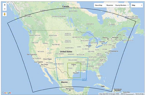
Simulation inputs were taken from the Texas Commission on Environmental Quality (TCEQ) Future Year 2017 Case, released December 5, 2016 (TCEQ 2016b), with 2012 meteorology simulated by the Weather Research and Forecasting (WRF) model (Skamarock et al. 2008) and 2017 emissions extrapolated from 2015 emissions provided by US EPA (2017b). To obtain the projected 2017 emissions for the power plants, the emissions for each hour of the day were averaged across every day of each month of 2015, to get a diurnal cycle of emissions that was applied to every day in the respective month (i.e., every day in January had the same emissions cycle, every day in February had the same emissions cycle, etc.). Then the NO_x emissions rates were increased by a scaling factor specific to each plant based on the effects of the Cross State Air Pollution Rule and the Emissions Banking and Trading Programs, but the SO₂ emissions were not. More detailed information on the development of these inputs and on the TCEQ model can be found in Chapters 2 and 3 of TCEQ (2016a). Variabilities in daily emissions rates at each power plant are shown in Figures SI1 and SI2.

All runs were conducted on a High Throughput Computing (HTC) Cluster of the Rice Big Research Data (BiRD) cloud infrastructure (80 dual processor HP SL230s nodes and 16 cores supporting two threads on each node). TCEQ evaluated its model for accuracy in both the meteorological data and ambient air pollution data for ozone and its precursors. Overall, the model outperformed EPA benchmarks for regulatory modeling, although it underpredicted some of the highest ozone peaks (TCEQ 2016a). Because the same inputs were used for this study, and because ozone concentrations did not change significantly with aerosol chemistry included, these model evaluations were sufficient to indicate that the model used in this study also performed adequately for meteorology and gas-phase pollutants.

Model evaluation

TCEQ’s simulation did not include aerosol processes needed to simulate PM_2.5. We conducted sensitivity tests that confirmed that our inclusion of the aerosol chemistry capabilities of CAMx did not substantially change ozone concentrations or their sensitivity to power-plant NO_x emissions. In order to evaluate the model performance in terms of PM_2.5, modeled concentrations averaged over all episode days for total PM_2.5 and major PM_2.5 species were compared to observed 2012 concentrations at monitors averaged in the same manner. The comparisons are imprecise, since the model used 2017 projected emissions with 2012 meteorology, whereas the observations are from 2012, but are the best available since TCEQ did not model PM in 2012. At the power plants considered here, SO₂ emissions declined by 13% and NO_x emissions by 18% from 2012 to 2017. However, PM precursors such as biogenic emissions were not affected by the projections. The model-simulated concentrations were moderately lower than the 2012 observations for total PM_2.5, sulfate, and ammonium (normalized mean bias [NMB] −13%, −31% and −9%, respectively), consistent with the reduction in SO₂ emissions. However, the model sharply underestimated nitrate (NMB −84%) (Table 1). Similar underestimates of nitrate have been documented in other summertime simulations (e.g., Morris et al. 2005; Tesche et al. 2006); nitrate was a small portion of total PM_2.5 observed at Texas monitors during the episode (0.31 – 0.41 µg/m³; 3 – 5%). Organic carbon evaluations were not quantified because of the uncertainty involved in scaling organic carbon measurements (El-Zanan et al. 2005), and because coal-fired power plants are not major sources of the hydrocarbons that form organic aerosols in Texas.

Table 1. Performance statistics for CAMx simulations of total and speciated PM_2.5, evaluated against observations at regulatory monitors.

	Total PM2.5	Nitrate	Sulfate	Ammonium
Mean bias	−1.4	−0.3	−0.8	−0.1
Mean error	3.5	0.3	0.8	0.3
Mean normalized bias	−22%	−84%	−30%	2%
Mean normalized error	27%	84%	30%	42%
Normalized mean bias	−13%	−84%	−31%	−9%
Normalized mean error	31%	84%	31%	40%
Mean fractional bias	−8%	−147%	−36%	−7%
Mean fractional error	48%	147%	36%	43%
Root mean square error	4.5	0.3	0.9	0.3

Note. For Mean Bias, Mean error, and Root mean square error, the units are µg/m³.

Unfortunately, estimating confidence intervals for responsiveness of ozone and PM_2.5 to precursor emissions in photochemical models is extraordinarily complex (e.g., Beddows et al. 2017; Digar, Cohan, and Bell 2011; Huang et al. 2017). Thus, uncertainty analysis of the CAMx model sensitivity results is beyond the scope of this study.

Air pollution episodes

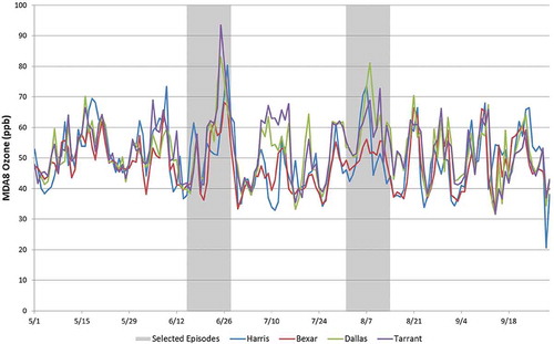
Modeling was conducted for two separate 2-week episodes, using WRF-simulated meteorology from June 15–20 and August 1–14, 2012 (Figure 2). These episodes were chosen based on high ozone concentrations in and around Harris, Bexar, Dallas, and Tarrant counties in the Base Case. These counties have the highest peak ozone concentrations in Texas and are thus the focus of regulatory efforts. Ozone concentrations during the episodes were 13–21% higher than observed during the full ozone season in these counties, and PM_2.5 concentrations were 17–20% higher than the annual averages (Table SI4).

Figure 2. Base Case modeled MDA8 ozone concentrations averaged within selected counties of Texas.

In addition to the simulation with “Base Case” projected 2017 emissions, each “zero-out” run was conducted by removing one of the 13 highest-emitting coal-fired power plants in the fine modeling domain. Zeroing out power plants one at a time is a reasonable approach since impacts of two plumes tend to be additive rather than nonlinear when interactions occur substantially downwind (Cohan et al. 2005), as is the case here. The capacity, generation, and emissions of those power plants are shown in Table 2. Information on control technologies for those power plants is shown in Table SI1.

Table 2. Capacities, generation, daily SO₂ and NO_x emissions (averaged over all episode days), and annual CO₂ emissions (2015 data) for coal-fired power plants in Texas (US EPA 2017b).

	Capacity (MW)	Annual generation (GWhr/yr)	Unscaled generation (GWhr/day)	Scaled generation (GWhr/day)	SO2 (tpd)	NOx (tpd)	CO2 (tpy)
Big Brown	1,208	8,200	24.7	20.3	141.6	13.6	8,900,000
Coleto Creek	635	3,400	12.7	14.6	29.3	8.5	3,400,000
Fayette Power Project	1,636	9,400	34.3	34.6	3.3	18.9	10,200,000
J K Spruce	1,350	4,800	20.2	25.0	1.9	11.2	5,200,000
J T Deely	840	3,900	15.7	24.3	38.6	12.4	4,300,000
Limestone	1,689	9,800	33.8	22.1	58.3	19.7	9,900,000
Martin Lake	2,455	11,000	40.7	31.6	70.6	27.3	12,500,000
Monticello	1,955	5,200	33.0	33.9	132.2	26.8	5,900,000
Oak Grove	1,665	12,800	39.8	46.8	11.5	16.2	13,200,000
San Miguel	391	2,400	7.9	6.2	17.2	5.6	3,100,000
Sandow	600	4,500	13.3	22.4	59.8	7.3	4,900,000
W A Parish	2,499	16,100	53.8	63.7	144.9	15.5	16,300,000
Welsh	1,584	4,200	14.8	11.3	34.1	11.2	4,600,000

Emissions

Emissions depend strongly upon control technologies. For example, SO₂ emissions per MWhr are more than an order of magnitude higher at the facilities that lack desulfurization devices (Big Brown, Coleto Creek, J T Deely, and Welsh) than at plants where all the units have wet scrubbers (Fayette, J K Spruce, and Oak Grove). At Monticello and W A Parish, only certain units are scrubbed and thus overall SO₂ emissions are high. Differences in NO_x emissions per MWhr are less extreme, since all of the power plants use some technologies to reduce NO_x emissions. However, the high-performing selective catalytic reduction devices at W A Parish, necessitated by its location within an ozone nonattainment region, enable it to emit a factor of 5 less NO_x per MWhr than the highest emitting power plants. We considered only smokestack emissions from coal combustion, neglecting the upstream emissions from coal mining and transport, which add about 6% to the greenhouse gas footprint (Venkatesh et al. 2012), and fugitive dust from the coal pile (Mueller et al. 2015).

Air quality impacts

Average impacts were determined by differencing the maximum daily 8-hr average (MDA8) ozone and daily 24-hr average (DA24) PM_2.5 concentrations across the fine domain, for each day of each episode, between the Base Case and each zero-out case. EPA has set ambient air quality standards at 70 ppb for fourth highest MDA8 ozone and 12 μg/m³ for annual average PM_2.5. Since this study did not simulate a whole year, the modeled changes to monitor concentrations do not translate perfectly to these regulatory limits, especially since high-ozone periods were chosen for the episodes (Table SI4), but they can indicate the scope of the expected impacts. The representativeness of episodes is especially a concern for ozone, due to the strongly nonlinear response of ozone concentrations to emissions.

For ozone, regulatory impacts were analyzed at the 26 monitors (Figure 3) for which the 2015 design values (DV) exceeded the 70 ppb MDA8 ozone standard. For each of these monitors, the effect of each zero-out case was measured as (1) the average decrease in the MDA8 ozone concentration across all days and (2) the maximum decrease in the MDA8 ozone concentration across all days.

Figure 3. Locations of monitors of interest and Class I areas.

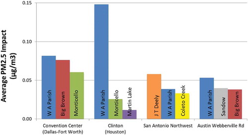
For PM_2.5, all Texas monitors attain the 12-μg/m³ annual standard, but it is possible that EPA could tighten the standard in the future. The World Health Organization sets a guideline value of 10 μg/m³ for annual PM_2.5 (http://www.who.int/mediacentre/factsheets/fs313/en), a level exceeded by some Texas monitors. Thus, for PM_2.5 we focus on effects at the one monitor in each of the four major Texas metropolitan areas (Dallas–Fort Worth, Houston, San Antonio, and Austin) that had the highest 2015 DV (Figure 3). For each of these monitors, the effect of each zero-out case was measured in two ways: (1) the average decrease in the PM_2.5 concentration across all days and (2) the maximum decrease in the DA24 PM_2.5 concentration across all days. Impacts of the power-plant plumes on particle-phase water were excluded.

Climate impacts

Climate impacts were assessed based on the CO₂ emissions rate of each power plant. Upstream emissions from coal mining and transport were not considered. We assumed a $52/short ton monetized social cost of CO₂ emissions, based on interpolating between the 2015 and 2020 estimates under a 3% discount rate from the Interagency Working Group on Social Cost of Greenhouse Gases (2016), and converting to 2017 dollars.

Visibility impacts

Changes in visibility at Class I Areas were evaluated using the IMPROVE algorithm (Pitchford et al. 2007). Class I Areas are a group of 158 national parks, fish and wildlife refuges, and Forest Service Wilderness Areas that were given the greatest level of air quality protection under the Clean Air Act in a 1977 amendment. In this study, effects on Big Bend National Park, Guadalupe Mountain National Park, Salt Creek Fish & Wildlife Refuge, Wichita Mountain Fish & Wildlife Refuge, and Caney Creek Forest Service Wilderness Area were considered (Figure 3). To determine the effects on visibility at each of these Class I Areas, the concentrations of each of the components of the IMPROVE equation were averaged for each episode. Then the IMPROVE equation was used to calculate average light extinction for each episode, using the hygroscopicity for that month (Pitchford et al. 2007). These values were then averaged and used to calculate a Haze Index (in deciview, dV) across both episodes. A visibility change of 1 dV is generally recognized to be humanly perceptible (US EPA 2016b).

BenMAP modeling of health impacts

Health impacts stemming from the changes in air quality were analyzed with BenMAP, using the same health impact and valuation functions as were used by US EPA (2015b) to determine and valuate mortality due to long-term exposure to PM_2.5 (Krewski et al. 2009; Lepeule et al. 2012) and short-term exposure to ozone (Smith, Baowei, and Switzer 2009; Zanobetti and Schwartz 2008) (see Table SI2 for details). For ozone, mortality of all ages was considered, but for PM_2.5, only adult mortality was considered because the studies used considered only adult mortality and, based on the results from US EPA (2015b), the impacts on infant mortality would be small in comparison. Note that effects from non-mortality-related impacts were not included in this analysis. Because not all impacts are included, our results are conservative estimates of total impacts. Because two health impact functions were used to calculate both ozone and PM_2.5 impacts, the two results were averaged to obtain the impact from each pollutant. Also, in order to capture the uncertainty in the impacts, we calculated the 95% confidence intervals (CIs) of the health impact functions and the valuation functions. We scaled the ozone impacts by 0.42, following the approach of Digar, Cohan, and Bell (2011), since we expect NO_x reductions to reduce ozone only during the 5-month ozone season. Ozone itself remains unhealthful throughout the year (Bell et al. 2004), but is insensitive to or even negatively correlated with NO_x when cool weather suppresses biogenic VOC emissions (Zhang et al. 2009; Luecken et al. 2018). We did not scale the PM_2.5 impacts, because NO_x and SO₂ contribute to PM_2.5 year-round, albeit with temporal variations that cannot be assessed here. Each of these impacts was also normalized based on daily-average generation (MWhr/day).

Because modeling episodes were chosen based on high ozone concentrations, it is possible that this scaling method overestimated ozone impacts (and, to a lesser extent, PM_2.5 impacts). However, these biases will be lessened by the facts that impacts were calculated based on changes in concentrations, rather than absolute concentrations, and that ozone and PM_2.5 concentrations during these episodes were just 13–21% higher than seasonal and annual averages, respectively (Table SI4).

Reduced-form modeling of health impacts

Reduced-form modeling was used to provide alternate estimates of the monetized mortality impacts of the power-plant emissions considered in the preceding. We obtained version 2 of APEEP (AP2) from its developer Nick Muller and adopted the updates described by Pourhashem et al. (2017). We obtained EASIUR from its developer Jinhyok Heo (http://barney.ce.cmu.edu/~jinhyok/easiur).

APEEP computes the ozone impacts of NO_x emissions and the PM impacts of NO_x and SO₂ emissions from each county and each of three emissions heights using a Gaussian plume model (Muller 2011; National Research Council 2010). Some applications of APEEP have tallied monetized impacts as an aggregate of marginal effects of emissions on mortality, morbidity, agriculture, visibility, and recreation (Muller 2014). Here, we considered only the premature mortality impacts, since they dominate other impacts on a monetized basis (U.S. EPA, 2011) and for consistency with EASIUR and BenMAP as applied here. APEEP considers impacts of short-term ozone exposure based on Bell et al. (2004), short-term PM_2.5 exposure based on Klemm and Mason (2003), and long-term PM_2.5 exposure based on Pope et al. (2002). EASIUR considers only the impacts of PM_2.5 exposure based on Krewski et al. (2009), which is the less responsive of the two functions averaged in the BenMAP analysis (Table SI4). We treated emissions from J K Spruce, San Miguel, Sandow, and Welsh as being released from medium stacks (250–500 m effective plume height) and the remainder from tall stacks (> 500 m effective plume height), following the recommendation of Nick Muller (personal communication, March 2018). APEEP does not simulate emissions from Oak Grove directly since it opened after 2008, so we use its estimates of marginal damages from emissions from its county at a medium plume height (250–500 m).

EASIUR considers only mortality impacts from PM_2.5 resulting from emissions in each grid cell (Heo et al. 2016). We applied EASIUR to NO_x and SO₂ emissions from each power plant, mapped to the corresponding EASIUR grid cell. EASIUR models emissions from ground-level, 150-m, and 300-m sources; we assumed a 300-m stack height for all plants. EASIUR computes source–receptor relationships using a tagged emissions version of the CAMx model. That provides a more comprehensive representation of atmospheric photochemistry than the Gaussian plume model used by APEEP, but limits meteorological inputs to a single year, 2005.

APEEP sets the value of a statistical life (VSL) at $6 million in 2000 USD (Muller 2014), and EASIUR at $8.6 million in 2010 USD (Heo, Adams, and Gao 2016). The user can choose the value of VSL in BenMAP. U.S. EPA (2015b) reviewed 26 published estimates of VSL and chose a central estimate of $10.0 million in 2011 USD based on projected 2024 income levels. To neutralize the effect of these assumptions on comparisons and to be roughly consistent with US EPA (2015b), we adjusted all values to a VSL of $10 million in 2016 USD.

Profitability assessment

Finally, we estimated the profitability of each power plant based on market conditions in 2016. The data used in this analysis were taken from SNL Financial’s online data portal. For fuel costs, we used plant-specific estimates reported by each plant or calculated by SNL. We assumed nonfuel variable operations and maintenance (O&M) costs equaled the 2016 average of the costs for Harrington, Tolk, Welsh, Pirkey, and Oklaunion power plants, since these plants are regulated entities and must therefore report these costs. Similarly, the annual capital expenses (Cap-ex) for each plant in this study were assumed to be equal to half of the average across those same five plants of the averaged 2006 to 2016 Cap-ex, which were calculated as the yearly difference between the “Total Cost” values in their FERC Form 1. This number was halved because it is likely that as these plants become less financially stable, they will put less money than in the past into Cap-ex, if at all possible, and that these plants have lower capital expenses than the regulated entities.

For revenues, ERCOT forward market prices were pulled from SNL Financial on July 24, 2017, and averaged across all ERCOT zones and then between on-peak and off-peak prices to obtain an overall monthly ERCOT market price for 2016. Monthly generation for each plant was taken as reported by SNL Financial. Using all of these data, a pretax earnings estimate for 2016 was calculated for each power plant.

Results and discussion

Climate impacts

CO₂ emission rates fell in a narrow range from 1.00 to 1.26 short tons/MWhr in 2015. These values are direct emissions from combustion, and do not consider the life cycle of coal mining and transport or power-plant construction. The range in CO₂ emission rates reflects the relative efficiencies of the power plants and the carbon content of their coal. None of the plants captured their carbon emissions in 2015, though W A Parish now captures CO₂ from a portion of the slipstream of one of its four units. San Miguel and Monticello had the highest emission rates (1.26 and 1.15 short tons/MWhr, respectively), in part due to their use of lignite, which has a lower heat content than other coal.

Ozone impacts

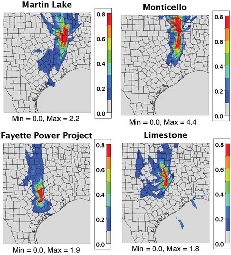
Ozone impacts were far more varied across the plants, due to their sharply different NO_x emissions and the spatial variability of ozone sensitivity to NO_x. Averaged over the fine domain, Martin Lake and Monticello formed the most ground-level ozone, about 0.06 ppb each (Table 5). As can be seen in Figure 4, ozone impacts were most intense in counties adjacent to the plants, and extended for hundreds of kilometers downwind.

Figure 4. Difference between MDA8 ozone in Base Case and power-plant zero-outs averaged over June episode for plants with high overall impacts (ppb).

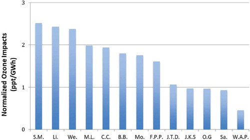
Normalized by daily generation, San Miguel, Limestone, and Welsh most strongly impacted ozone, with impacts near 2.5 ppt/GWhr. Impacts were below 1 ppt/GWhr for four other power plants (Figure 5), reflecting their lower NO_x emission rates (Table 2).

Figure 5. Impacts on MDA8 ozone averaged over all days and over the fine-scale domain and normalized by daily GWhr.

As expected, the power plants closest to each of the three main metropolitan areas (Dallas–Fort Worth, Houston, and San Antonio) tended to have the greatest effects on regulatory monitors in those regions (Figure 6).

Figure 6. Three largest impacts on MDA8 ozone averaged over all days at the monitors with the highest design values in the (a) Dallas–Fort Worth, (b) Houston, and (c) San Antonio regions.

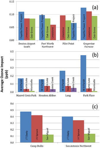
In the Dallas–Fort Worth region, averaged over the episodes, Limestone had the greatest impact on a single monitor (0.17 ppb at Dallas Hinton), while Fayette Power Project had the greatest impact on the most monitors (7 of the 12). Monticello had the greatest impact on a monitor on a single day (1.7 ppb at Dallas Hinton). At all four of the monitors with the highest ozone design value, Fayette Power Project, Limestone, and Oak Grove had the largest impacts (Figure 6).

In the Houston region, W A Parish had the largest impact on episode-average ozone at 10 of the 12 monitors examined, including 0.48 ppb at Houston Croquet. Its peak single-day MDA8 ozone impact was 3.3 ppb at the Northwest Harris County monitor. The large ozone impacts reflect the proximity of W A Parish in the southwest corner of the Houston region and its large size, despite its stringent NO_x control from selective catalytic reduction. W A Parish had by far the largest impacts, followed by Martin Lake, on all four of the monitors with the highest DV (Figure 6).

In the San Antonio region, the nearby J T Deely had the most impact on episode-average ozone at both monitors, including 0.48 ppb at Camp Bullis. Two other nearby power plants, J K Spruce and San Miguel, ranked second and third. J K Spruce had the largest single-day ozone impact, 1.5 ppb at San Antonio Northwest.

In each region, daily variations in power-plant impacts were not significantly correlated with daily ozone concentrations. In other words, power plants did not have a consistently larger impact on high-ozone days than on average- or low-ozone days.

PM_2.5 impacts

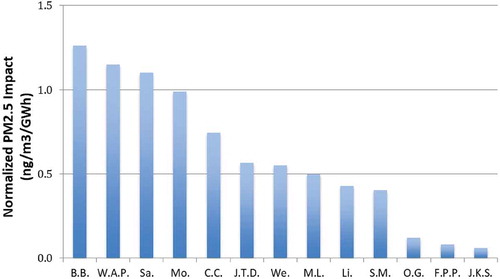
As with ozone, PM_2.5 impacts varied widely across the plants. Averaged over the fine domain and episodes, the largest amounts of PM_2.5 formed from W A Parish (0.06 μg/m³), Monticello (0.03 μg/m³), Big Brown (0.03 μg/m³), and Martin Lake (0.02 μg/m³) (Table 5). These four plants were also the largest SO₂ emitters (Table 2). All other plants had PM_2.5 impacts below 0.015 μg/m³. Normalized by daily generation, Big Brown had the largest domain-wide impact (1.3 ng/m³/GWhr) (Figure 8).

Figure 7. Difference between PM_2.5 in Base Case and power-plant zero-outs averaged over June episode for plants with high overall impacts (µg/m³).

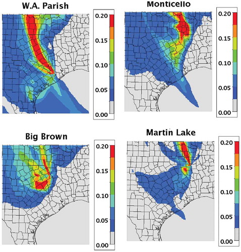
Figure 8. Impacts on PM_2.5 averaged over all days and over the fine-scale domain and normalized by daily GWhr.

As shown in Figure 9, though located in the Houston region, W A Parish had the largest episode-average impact on PM_2.5 not only at the most polluted monitor in the Houston region (Clinton; 0.15 μg/m³), but also in the Dallas–Fort Worth region (Convention Center; 0.08 μg/m³) and Austin region (Austin Webberville Road; 0.05 μg/m³). In the San Antonio region, nearby J T Deely had the largest impact at its most polluted monitor (San Antonio Northwest; 0.06 μg/m³). After normalizing by daily generation, though, Sandow had the largest impact in Dallas–Fort Worth and Austin (3.8 and 3.0 ng/m³/GWhr, respectively), while W A Parish remained the most important in Houston and J T Deely in San Antonio (2.8 and 3.7 ng/m³/GWhr, respectively).

Figure 9. The three largest impacts from power plants on PM_2.5 averaged over all days at the monitor in each region with the highest PM_2.5 design value.

In terms of maximum daily impacts, Monticello had the greatest effect in Dallas–Fort Worth (0.43 μg/m³), W A Parish in Houston (0.92 μg/m³), Coleto Creek in San Antonio (0.47 μg/m³), and Big Brown in Austin (0.40 μg/m³).

Visibility impacts

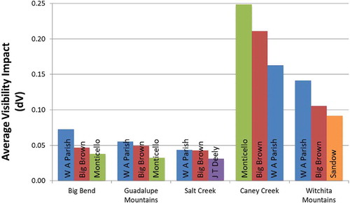
As shown in Figure 10, among the Class I Areas on an episode-average basis, Caney Creek was most impacted by the power plants—0.25 dV from Monticello, 0.21 dV from Big Brown, 0.16 dV from Parish, and 0.12 dV from Martin Lake. Since 1 dV is recognized as humanly perceptible (US EPA 2016b), these collective impacts can be substantial, especially on days with higher than average impacts. In the Wichita Mountains, average impacts were 0.14 dV from Parish and 0.11 dV from Big Brown. For all other Class I Areas, impacts from individual power plants were below 0.1 dV. This does not necessarily rule out concern about haze impacts in those other areas, since there could be impacts on peak days during nonsummer months.

Figure 10. The three largest impacts from power plants on visibility at each Class I area, averaged over all episode days.

Health impacts

The air quality impacts computed by CAMx were input into BenMAP to compute resulting impacts on health. BenMAP provides results both in terms of increased mortality and associated monetized impacts, with valuation set at approximately $10 million per death. The 95% CI ranges represent uncertainty only in the health impact functions and valuation functions within BenMAP, because uncertainties of photochemical model outputs from CAMx cannot be readily computed.

Overall in the CAMx/BenMAP modeling, power-plant mortality impacts via PM_2.5 were more than an order of magnitude larger than those via ozone (Table 5). Martin Lake and Limestone created the most health effects due to ozone (1.1 [0.4–2.0] and 1.0 [0.4–1.9] deaths/yr, respectively), whereas W A Parish and Big Brown had the greatest effects from PM_2.5 (177 [77–353] and 81 [35–162] deaths/yr, respectively). The top five most impactful plants for each pollutant are shown in Table 3.

Table 3. Power plants with the five largest impacts on mortality summed over the fine-scale domain, as computed by CAMx/BenMAP. Values in parentheses are 95% CIs of health impact functions.

	Normalization
	None (deaths/year)	Generation (deaths/TWhr)
MDA8 Ozone	Martin Lake	San Miguel
	1.1	0.13
	(0.4, 2.0)	(0.05, 0.24)
	Limestone	Limestone
	1.0	0.13
	(0.4, 1.9)	(0.05, 0.23)
	W A Parish	Big Brown
	1.0	0.1
	(0.4, 1.8)	(0.04, 0.18)
	Monticello	J T Deely
	0.9	0.1
	(0.4, 1.7)	(0.04, 0.17)
	Fayette Power Project	Welsh
	0.9	0.1
	(0.4, 1.7)	(0.04, 0.17)
PM2.5	W A Parish	Sandow
	177	9.1
	(77, 353)	(4.0, 18.1)
	Big Brown	Big Brown
	81	9.0
	(35, 162)	(3.9, 18.0)
	Monticello	W A Parish
	76	9.0
	(33, 152)	(3.9, 18.0)
	Sandow	Monticello
	44	6.3
	(19, 88)	(2.8, 12.6)
	Martin Lake	J T Deely
	41	5.1
	(18, 83)	(2.2, 10.2)

Table 4. Estimated variable O&M costs and pretax earnings in 2016 for power plants in Texas.

	Variable O&M ($/MWhr)	Pretax earnings (million $)	Pretax earnings ($/MWhr)
Sandow	17.41	−1.7	−0.44
Coleto Creek	25.11	−25.1	−8.04
Oak Grove	19.75	−29.2	−2.41
Limestone	20.88	−46.8	−5.11
Big Brown	24.03	−49.0	−7.80
Martin Lake	19.98	−49.3	−4.39
J T Deely	33.62	−53.7	−22.11
San Miguel	43.67	−63.8	−27.15
Welsh	31.42	−75.4	−16.80
Monticello	26.52	−89.4	−11.87
J K Spruce	31.93	−91.3	−16.76
Fayette	26.65	−100.3	−9.88
W A Parish	25.99	−124.2	−9.87

Table 5. Results of the six main impact metrics (maximum MDA8 ozone, average MDA8 ozone, maximum DA24 PM_2.5, average DA24 PM_2.5, mortality from ozone, mortality from PM_2.5) for each of the 13 power plants of interest in CAMx/BenMAP modeling.

	Maximum MDA8 ozone (ppb)	Average MDA8 ozone (ppb)	Maximum DA24 PM2.5 (μg/m^3)	Average DA24 PM2.5 (μg/m^3)	Ozone health (deaths)	PM2.5 health (deaths)
Big Brown	2.1	0.04	0.5	0.031	1	81
Coleto Creek	1.7	0.03	0.2	0.009	0	22
Fayette Power Project	2.2	0.06	0.1	0.003	1	7
J K Spruce	0.7	0.02	0.1	0.001	1	5
J T Deely	0.7	0.03	0.1	0.009	1	29
Limestone	1.8	0.05	0.2	0.014	1	41
Martin Lake	2.9	0.06	0.5	0.020	1	42
Monticello	4.4	0.06	1.0	0.033	1	76
Oak Grove	1.6	0.05	0.2	0.005	1	15
San Miguel	1.2	0.02	0.1	0.003	0	7
Sandow	1.4	0.02	0.6	0.015	1	44
W A Parish	1.0	0.03	1.2	0.062	1	177
Welsh	2.2	0.03	0.2	0.008	0	18

Note. Maximum refers to the grid cell with the maximum impacts after averaging over all days.

After normalizing by generation, San Miguel and Limestone had the largest estimated impacts from ozone (0.13 [0.05–0.24] and 0.13 [0.05–0.23] deaths/TWhr, respectively) and Sandow, Big Brown, and W A Parish had the largest impacts from PM_2.5 (9.1 [4.0–18.1], 9.0 [3.9–18.0], and 9.0 [3.9–18.0] deaths/TWhr, respectively). The rankings result from relatively high SO₂ emission rates and, for W A Parish, proximity to Houston.

When considering the value of the impacts from both ozone and PM_2.5, the largest normalized health impacts (Sandow, Big Brown, and W A Parish) each correspond to a monetized value of approximately $90/MWhr. Each of these plants emitted large amounts of SO₂ upwind of populated areas. By contrast, power plants with modern SO₂ controls such as Fayette, J K Spruce, and Oak Grove (Table SI1) caused health impacts of roughly $10/MWhr. For comparison, Levy, Baxter, and Schwartz (2009) reported a range of $20 to $1,570/MWhr as the health effects associated with electricity generation from coal across U.S. power plants.

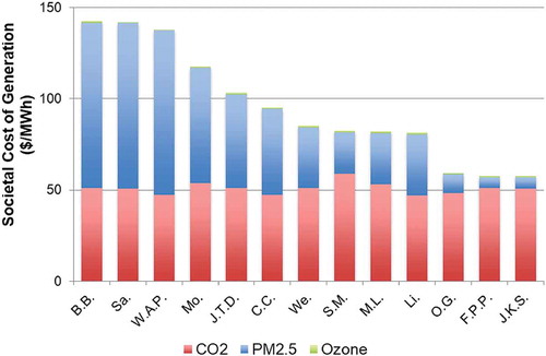
Significant additional monetary impacts are realized when considering the social cost of CO₂ emissions. Using a social cost of carbon of $52/short ton (in 2017 dollars), climate impacts range from $47/MWhr at Limestone to $59/MWhr at San Miguel. This narrow range reflects the relatively uniform rates of CO₂ emissions compared to the starkly divergent SO₂ emission rates.

Combining all societal impacts (Figure 11), Big Brown and Sandow had the largest impacts ($143/MWhr), while all of the 13 plants had impacts above $57/MWhr. That is far higher than the average wholesale cost of electricity in ERCOT, which was just $22/MWhr in 2016, according to data from SNL Financial.

Figure 11. Societal costs of generation for each power plant, based on a $52/ton social cost of CO₂ and the mortality impacts of PM_2.5 and ozone.

The reduced-form models APEEP and EASIUR provide alternatives to CAMx/BenMAP for computing monetized health impacts. For ozone, CAMx/BenMAP estimates an impact of $0.85/MWhr averaged across the power plants, whereas APEEP (normalized to a $10 million VSL) estimates $0.23/MWhr. This difference likely arises from the use of high ozone episodes in CAMx and annual conditions in APEEP. EASIUR does not model ozone. For PM_2.5, CAMx/BenMAP estimates $44/MWhr, APEEP estimates $30/MWhr, and EASIUR estimates $42/MWhr. The lower estimates from APEEP may result in part from its use of a relatively simple Gaussian plume model rather than the more sophisticated representation of photochemistry in CAMx and EASIUR.

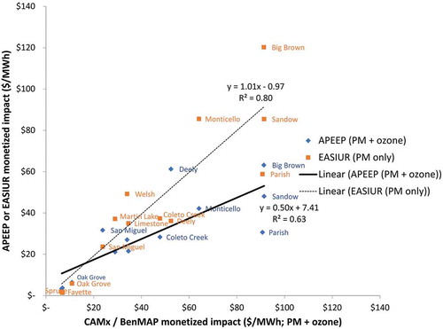
Comparing individual power-plant impacts across the three methods, the coefficient of determination between EASIUR and CAMx/BenMAP results was R² = 0.80, and between APEEP and CAMx/BenMAP it was R² = 0.63 (Figure 12). The methods consistently ranked several power plants (e.g., Big Brown) as having the largest impacts on health per MWhr, and certain other plants (e.g., J K Spruce) having an order of magnitude smaller effect. One notable difference is that EASIUR indicated a large spread between the per-MWhr health impacts of Big Brown, Sandow, and W A Parish, whereas CAMx/BenMAP computed a narrower spread (Figure 12). That is because CAMx modeled the W A Parish plume to frequently impact densely populated areas in the nearby Houston suburbs and the Dallas–Fort Worth region downwind during the episodes (Figure 7), counteracting its lower per-MWhr emissions rate (Table 2). The coarse modeling of EASIUR muted the spatial differences of plume locations and population density, and thus found per-MWhr health impacts that more closely resembled the spread in per-MWhr emissions.

Figure 12. Monetized mortality impacts from each power plant simulated by APEEP or EASIUR compared to the results from CAMx/BenMAP.

Note that the EASIUR results exclude ozone, but that ozone represents a small portion of the CAMx/BenMAP and APEEP monetized impacts. Also, note in Table SI2 that EASIUR uses only the less responsive one (Krewski et al. 2009) of the two PM_2.5 concentration-response functions considered in our application of BenMAP (Krewski et al. 2009; Lepeule et al. 2012); scaling the EASIUR results by a factor of 1.62 would normalize for that difference. The form of the PM_2.5 concentration-response function embedded into APEEP (Pope et al. 2002; Table SI3) differs from the ones used by BenMAP and EASIUR, and thus cannot be readily scaled to match the others.

Profitability analysis

Our analysis of power prices, fuel and other operating and maintenance costs, and discounted capital expenses indicates that none of the 13 coal-fired power plants earned a net profit in 2016 (Table 4). Our estimates of net cash flow range from –$1.7 million at Sandow to –$124.2 million at W A Parish. Normalized by 2016 generation, losses ranged from $0.44/MWhr at Sandow to $27.15/MWhr at San Miguel. The range reflects the much lower variable O&M costs for Sandow ($17.41/MWhr) than for San Miguel ($43.67/MWhr). Note that 9 of the 13 power plants had fuel and other variable O&M costs that were, by themselves, more expensive than the average ERCOT market price for 2016 as reported by SNL Financial ($22.10/MWhr).

It is possible that the closure of some of these plants will lead to an increase in the ERCOT market price, which could improve the financial situations of the plants that did not close. This will become apparent in 2018, when four of the plants considered here (Monticello, Big Brown, Sandow, and J T Deely) will close. That may be why other plants have not closed already, despite their likely negative cash flows. However, it is also possible that increased generation during this time period, namely, from natural gas and renewables, will negate some or all of the positive effects of coal plant closures on the finances of other coal plants.

Conclusion

Our results show fairly similar climate impacts from each coal-fired power plant but an order of magnitude range in impacts on ozone and PM_2.5, both at regulatory monitors and on a health or visibility basis, after normalizing by daily generation. Differing emissions control technologies and proximity to urban areas drove the differences in health impacts, while the narrow range of efficiencies drove the similarities in CO₂ emissions.

Ozone impacts may be overstated because the episodes modeled included periods of high ozone concentrations, although the differences from seasonal averages were modest (Table SI4). Since ozone represents a small portion of overall monetized valuations (Figure 11), the effect of episode selection bias on aggregate impacts will be muted.

Another caveat is that all of our health impacts modeling apply what the Health Effects Institute calls a “chain of accountability” to link emissions with ambient air quality, exposure, and ultimately human health responses (Health Effects Institute 2003). Each link in this chain compounds uncertainty. For example, the historical concentration-response functions computed by epidemiological studies in other regions will not precisely represent conditions in Texas today.

We find that health impacts are more variable and in some cases larger than climate impacts on a monetized basis. In particular, power plants that do not scrub their sulfur are most damaging to health and visibility via impacts on particulate sulfate. Setting policy solely based on carbon emissions may mean foregoing opportunities to accelerate progress on air quality, health, and visibility. Our finding that particulate matter imposes the greatest impact on human health is consistent with other studies (Fann et al. 2012; Pope and Dockery 2006).

Sulfur emissions and associated PM_2.5 have received less attention in Texas than ozone-forming NO_x, because the state’s largest urban areas violate ambient standards for ozone but not for PM_2.5. In fact, TCEQ regulatory modeling does not even simulate formation of PM_2.5, requiring us to reactivate this standard feature of the CAMx model to conduct our analysis. While PM_2.5 modeling may be unnecessary for ozone attainment planning, our results suggest that PM_2.5 formation from SO₂ emissions is the leading cause of health impacts.

Our findings highlight opportunities for modeling to inform policies that would enhance societal outcomes as the Texas power market evolves. For now, power-plant closure decisions are based almost exclusively upon financial considerations of the facility owner, emitting pollution virtually for free within permitted limits. With health impacts per MWhr varying by an order of magnitude across facilities, policies targeting sulfur emissions and to a lesser extent NO_x could spur closures or emissions abatement at the facilities most potent at forming air pollution and associated health and visibility impacts. Since it will take a number of years before natural gas and renewable energy can fully replace coal on the Texas grid, such policies could accelerate the air quality and health benefits of the ongoing transition from coal to cleaner sources of electricity.

A missed opportunity for accelerating those benefits came with the reversal of the Regional Haze plan issued by EPA for Texas at the end of the Obama Administration (US EPA 2016b). That plan would have required SO₂ controls at eight of the highest emitting power plants considered here. Given the poor financial status of those plants as indicated by our study, such a plan would likely have prompted most of those plants to close or convert to natural gas, yielding substantial benefits for climate, air quality, and health beyond the stated purpose of reducing regional haze. Instead, EPA in 2017 replaced the plan with a cap-and-trade scheme, setting the cap higher than emissions in recent years (2018b; US EPA 2017c). That will allow several power plants to continue operating unscrubbed, resulting in monetized health impacts that far exceed the market price for their electricity.

Future work could compare the multifaceted impacts of power plants elsewhere. Dispatch modeling would be needed to explore how closures of some plants might lead to a rebound in utilization of remaining plants. Also, because PM_2.5 and associated regional haze affect health and visibility year-round, it will be important to model conditions outside the summer ozone season. The correlation between results from the CAMx/BenMAP, APEEP, and EASIUR approaches suggests that both regional photochemical modeling and reduced-form models are options for informing decision making, though further study is needed to compare the methods in other regions and time periods. Though EASIUR has a shorter track record than APEEP, its more advanced photochemical modeling and closer agreement with our direct modeling (Figure 12) suggest that it deserves more attention in future reduced-form modeling studies.

Acknowledgment

The authors acknowledge David Schlissel from IEEFA for his assistance in the profitability analyses and Jim MacKay, Ron Thomas, Miranda Kosty, and others in the Texas Commission on Environmental Quality Air Modeling Division for their assistance in obtaining, analyzing, and interpreting modeling inputs. The authors thank Nick Muller and Jinhyok Heo for making the AP2 and EASIUR models publically available.

Supplemental data

Supplemental data for this paper can be accessed on the publisher’s website.

Additional information

Funding

This work was supported by the National Aeronautics and Space Administration [NNX15AN63G].

Notes on contributors

Brian Strasert

Brian Strasert is an environmental engineer with GSI Environmental in Houston, TX, and a former M.S. candidate at Rice University in Houston, TX.

Su Chen Teh

Su Chen Teh is an undergraduate student at Rice University.

Daniel S. Cohan

Daniel S. Cohan is an associate professor of civil and environmental engineering at Rice University.

References

- Baker, K. R., R. A. Kotchenruther, and R. C. Hudman. 2016. Estimating ozone and secondary PM2.5 impacts from hypothetical single source emissions in the central and eastern United States. Atmos. Pollut. Res. 7 (1):122–133. doi:10.1016/j.apr.2015.08.003.
- Beddows, A. V., N. Kitwiroon, M. L. Williams, and S. D. Beevers. 2017. Emulation and sensitivity analysis of the community multiscale air quality model for a UK Ozone pollution episode. Environ. Sci. Technol. 51 (11):6229–6236. doi:10.1021/acs.est.6b05873.
- Bell, M. L., A. McDermott, S. L. Zeger, J. M. Samet, and F. Dominici. 2004. Ozone and short-term mortality in 95 US urban communities, 1987 – 2000. J. Am. Med. Assoc. 292 (19):2372–2378. doi:10.1001/jama.292.19.2372.
- Bergin, M. S., A. G. Russell, M. T. Odman, D. S. Cohan, and W. L. Chameides. 2008. Single-source impact analysis using 3D air quality models. J. Air Waste Manage. Assoc. 58 (10):1351–1359. doi:10.3155/1047-3289.58.10.1351.
- Byun, D., and K. L. Schere. 2006. Review of the governing equations, computational algorithms, and other components of the Models-3 community multiscale air quality (CMAQ) modeling system. Appl. Mechanics Rev. 59:51–77. doi:10.1115/1.2128636.
- Chang, J. S., R. A. Brost, I. S. A. Isaksen, S. Madronich, P. Middleton, W. R. Stockwell, and C. J. Walcek. 1987. A three-dimensional Eulerian acid deposition model: Physical concepts and formulation. J. Geophys. Res: Atmos 92 (D12):14681–14700. doi:10.1029/JD092iD12p14681.
- Cohan, D. S., A. Hakami, Y. Hu, and A. G. Russell. 2005. Nonlinear response of ozone to emissions: Source apportionment and sensitivity analysis. Environ. Sci. Technol. 39:6739–6748. doi:10.1021/es048664m.
- Cohan, D. S., D. Tian, Y. Hu, and A. G. Russell. 2006. Control strategy optimization for attainment and exposure mitigation: Case study for ozone in Macon, Georgia. Environ. Manage 38:451–462. doi:10.1007/s00267-005-0226-y.
- Cohan, D.S., J.W. Boylan, A. Marmur, and M.N. Khan. 2007. An integrated framework for multi-pollutant air quality management and its application in Georgia. Environmental Management 40:545-554.
- Digar, A., D. S. Cohan, and M. L. Bell. 2011. Uncertainties influencing health-based prioritization of ozone abatement options. Environ. Sci. Technol. 45 (18):7761–7767. doi:10.1021/es200165n.
- EIA. 2018. Energy-Related carbon dioxide emissions at the State Level, 2000-2015. Accessed https://www.eia.gov/environment/emissions/state/analysis/pdf/stateanalysis.pd
- El-Zanan, H. S., D. H. Lowenthal, B. Zielinska, J. C. Chow, and N. Kumar. 2005. Determination of the organic aerosol mass to organic carbon ratio in IMPROVE samples. Chemosphere 60 (4):485–496. doi:10.1016/j.chemosphere.2005.01.005.
- Fann, N., A. D. Lamson, S. C. Anenberg, K. Wesson, D. Risley, and B. J. Hubbell. 2012. Estimating the national public health burden associated with exposure to ambient PM2.5 and ozone. Risk Anal. 32 (1):81–95. doi:10.1111/j.1539-6924.2011.01630.x.
- Fann, N., C. M. Fulcher, and B. J. Hubbell. 2009. The influence of location, source, and emission type in estimates of the human health benefits of reducing a ton of air pollution. Air Qual. Atmos. Health 2 (3):169–176. doi:10.1007/s11869-009-0044-0.
- Health Effects Institute. 2003.Assessing health impact of air quality regulations: concepts and methods for accountability research. HEI Commun. 11. Accessed November 10, 2018 https://www.healtheffects.org/system/files/Comm11.pdf.
- Heo, J., P. J. Adams, and H. O. Gao. 2016. Public health costs of primary PM2.5 and inorganic PM2.5 precursor emissions in the United States. Environ. Sci. Technol. 50:6061–6070. doi:10.1021/acs.est.5b06125.
- Hildebrandt Ruiz, L., and G. Yarwood 2013. Interactions between organic aerosol and NOy: Influence on oxidant production (AQRP Project 12-012). Texas Air Quality Research Program. Accessed http://aqrp.ceer.utexas.edu/projectinfoFY12_13/12-012/12-012%20Final%20Report.pdf
- Huang, Z., Y. Hu, J. Zheng, Z. Yuan, A. G. Russell, J. Ou, and Z. Zhong. 2017. A new combined stepwise-based high-order decoupled direct and reduced-form method to improve uncertainty analysis in PM2.5 Simulations. Environ. Sci. Technol. 51 (7):3852–3859. doi:10.1021/acs.est.6b05479.
- Hubbell, B. J., N. Fann, and J. I. Levy. 2009. Methodological considerations in developing local-scale health impact assessments: Balancing national, regional, and local data. Air Qual. Atmos. Health 2:99–110. doi:10.1007/s11869-009-0037-z.
- IEEFA. 2016. The beginning of the end: Fundamental changes in energy markets are undermining the financial viability of coal-fired power plants in Texas. IEEFA. Accessed http://ieefa.org/wp-content/uploads/2016/09/The-Beginning-of-the-End_September-2016.pdf
- Interagency Working Group on Social Cost of Greenhouse Gases 2016. Technical support document: Technical update of the social cost of carbon for regulatory impact analysis under executive order 12866. Accessed https://obamawhitehouse.archives.gov/sites/default/files/omb/inforeg/scc_tsd_final_clean_8_26_16.pdf
- Karamchandani, P., and C. Seigneur. 1999. Simulation of sulfate and nitrate chemistry in power plant plumes. J. Air Waste Manage. Assoc. 49 (9):175–181. doi:10.1080/10473289.1999.10463885.
- Klemm, R. J., and R. Mason. 2003. Replication of reanalysis of harvard six-city mortality study. In Revised Analyses of Time-Series Studies of Air Pollution and Health, Health Effects Institute, Accessed https://www.healtheffects.org/system/files/TimeSeries.pdf.
- Krewski, D., M. Jerrett, R. T. Burnett, R. Ma, E. Hughes, Y. Shi, M. C. Turner, C. A. Pope III, G. Thurston, E. E. Calle; et al. 2009. Extended follow-up and spatial analysis of the American Cancer Society study linking particulate air pollution and mortality, Research Report 140; Health Effects Institute: Boston, MA.
- Lepeule, J., F. Laden, D. Dockery, and J. Schwartz. 2012. Chronic exposure to fine particles and mortality: An extended follow-up of the harvard six cities study from 1974 to 2009. Environ. Health Perspect. 120 (7):965–970. doi:10.1289/ehp.1104660.
- Levy, J. I., L. K. Baxter, and J. Schwartz. 2009. Uncertainty and variability in health-related damages from coal-fired power plants in the United States. Risk Analysis: Int. J. 29 (7):1000–1014. doi:10.1111/risk.2009.29.issue-7.
- Lim, S. S., T. Vos, A. D. Flaxman, G. Danaei, K. Shibuya, H. Adair-Rohani, … M. Ezzati. 2012. A comparative risk assessment of burden of disease and injury attributable to 67 risk factors and risk factor clusters in 21 regions, 1990–2010: A systematic analysis for the Global Burden of Disease Study 2010. Lancet 380 (9859):2224–2260. doi:10.1016/S0140-6736(12)61766-8.
- Luecken, D. J., S. L. Napelenok, M. Strum, R. Scheffe, and S. Phillips. 2018. Sensitivity of ambient atmospheric formaldehyde and ozone to precursor species and source types across the United States. Environ. Sci. Technol. 52 (8):4668–4675. doi:10.1021/acs.est.7b05509.
- Luminant. 2017a, October 6. Luminant announces decision to retire its monticello power plant. Accessed December 3, 2017 https://www.luminant.com/luminant-announces-decision-retire-monticello-power-plant/
- Luminant. 2017b, October 13. Luminant to close two Texas power plants. Accessed December 3, 2017 https://www.luminant.com/luminant-close-two-texas-power-plants/
- Moody’s Investors Service. 2016. ERCOT: Renewables to hold down power prices in the lone star State. Moody’s Investors Service. Accessed https://assets.documentcloud.org/documents/3022115/Moody-s-Report-on-Coal-Plants-in-ERCOT.pdf
- Morris, R. E., D. E. McNally, T. W. Tesche, G. Tonnesen, J. W. Boylan, and P. Brewer. 2005. Preliminary evaluation of the community multiscale air quality model for 2002 over the Southeastern United States. J. Air Waste Manage. Assoc. 55 (11):1694–1708. doi:10.1080/10473289.2005.10464765.
- Mueller, S. F., J. W. Mallard, Q. Mao, and S. L. Shaw. 2015. Emission factors for fugitive dust from bulldozers working on a coal pile. J. Air Waste Manage. Assoc. 65 (1):27–40. doi:10.1080/10962247.2014.960953.
- Muller, N. Z. 2011. Linking policy to statistical uncertainty in air pollution damages. B E J. Econom. Anal. Policy 11 (1): Article 32. doi:10.2202/1935-1682.2925.
- Muller, N. Z. 2014. Boosting GDP Growth by Accounting for the Environment. Science 345 (6199):873–874. doi:10.1126/science.1253506.
- Muller, N. Z., and R. Mendelsohn. 2007. Measuring the damages of air pollution in the United States. J. Environ. Econ. Manage 54 (1):1–14. doi:10.1016/j.jeem.2006.12.002.
- National Research Council. 2010. Hidden costs of energy: Unpriced consequences of energy production and use. Washington, DC: The National Academies Press.
- Nenes, A., S. N. Pandis, and C. Pilinis. 1998. ISORROPIA: A new thermodynamic equilibrium model for multiphase multicomponent inorganic aerosols. Aquatic Geochem. 4 (1):123–152. doi:10.1023/A:1009604003981.
- Nenes, A., S. N. Pandis, and C. Pilinis. 1999. Continued development and testing of a new thermodynamic aerosol module for urban and regional air quality models. Atmos. Environ. 33 (10):1553–1560. doi:10.1016/S1352-2310(98)00352-5.
- Odman, M. T., Y. Hu, A. Unal, A. G. Russell, and J. W. Boylan. 2007. Determining the sources of regional haze in the southeastern United States using the CMAQ model. J. Appl. Meteorology Climatol. 46 (11):1731–1743. doi:10.1175/2007JAMC1430.1.
- Pinder, R. W., R. L. Dennis, and P. V. Bhave. 2008. Observable indicators of the sensitivity of PM2.5 nitrate to emission reductions - Part I: Derivation of the adjusted gas ratio and applicability at regulatory-relevant time scales. Atmos. Environ. 42 (6):1275–1286. doi:10.1016/j.atmosenv.2007.10.039.
- Pitchford, M., W. Malm, B. Schichtel, N. Kumar, D. Lowenthal, and J. Hand. 2007. Revised algorithm for estimating light extinction from IMPROVE particle speciation data. J. Air Waste Manage. Assoc. 57 (11):1326–1336. doi:10.3155/1047-3289.57.11.1326.
- Pope, C. A., III, and D. W. Dockery. 2006. Health effects of fine particulate air pollution: Lines that connect. J. Air Waste Manage. Assoc. 56 (6):709–742. doi:10.1080/10473289.2006.10464485.
- Pope, C. A., III, R. T. Burnett, M. J. Thun, E. E. Calle, D. Krewski, K. Ito, and G. D. Thurston. 2002. Lung cancer, cardiopulmonary mortality, and long-term exposure to fine particulate air pollution. J. Am. Med. Assoc. 287 (9):1132–1141. doi:10.1001/jama.287.9.1132.
- Pourhashem, G., Q. Z. Rasool, R. Zhang, K. B. Medlock, D. S. Cohan, and C. A. Masiello. 2017. Valuing the air quality effects of biochar reductions on soil NO emissions. Environ. Sci. Technol. 51:9856–9863. doi:10.1021/acs.est.7b00748.
- Ryerson, T. B., M. Trainer, J. S. Holloway, D. D. Parrish, L. G. Huey, D. T. Sueper, G. J. Frost, S. G. Donnelly, S. Schauffler, E. L. Atlas, W. C. Kuster, P. D. Goldan, G. Hübler, J. F. Meagher, and F. C. Fehsenfeld. 2001. Observations of Ozone formation in power plant plumes and implications for ozone control strategies. Science 292 (5517):719–723. doi:10.1126/science.1058113.
- Skamarock, W. C., J. B. Klemp, J. Dudhia, D. O. Gill, D. M. Barker, M. G. Duda, X.-Y. Huang, W. Wang, and J. G. Powers, 2008: A description of the advanced research WRF Version 3. NCAR Tech. Note NCAR/TN-475+STR, 113 pp. doi:10.5065/D68S4MVH.
- Smith, R. L., X. Baowei, and P. Switzer. 2009. Reassessing the relationship between ozone and short-term mortality in U.S. urban communities. Inhal. Toxicol 21:37–61. doi:10.1080/08958370903161612.
- Strader, R., F. Lurmann, and S. N. Pandis. 1999. Evaluation of secondary organic aerosol formation in winter. Atmos. Environ. 33 (29):4849–4863. doi:10.1016/S1352-2310(99)00310-6.
- TCEQ. 2016a. Houston-galveston brazoria attainment demonstration State implementation plan revision for the 2008 Eight-Hour Ozone standard nonattainment area. Accessed https://www.tceq.texas.gov/assets/public/implementation/air/sip/hgb/HGB_2016_AD_RFP/AD_Adoption/16016SIP_HGB08AD_ado.pdf
- TCEQ. 2016b, December 5. TCEQ Future Year 2017 Case Files. Accessed ftp://amdaftp.tceq.texas.gov/pub/TX/camx/2012/fy17_12xxx.c0m_c0m.2012_wrf371_p2ma_i2mSNgqsfc0_f/
- Tesche, T. W., R. Morris, G. Tonnesen, D. McNally, J. Boylan, and P. Brewer. 2006. CMAQ/CAMx annual 2002 performance evaluation over the eastern US. Special Issue Model Evaluation: Evaluation Urban Regional Eulerian Air Quality Models 40 (26):4906–4919. doi:10.1016/j.atmosenv.2005.08.046.
- U.S. EPA. 2018b. Promulgation of air quality implementation plans; State of Texas; Regional Haze and interstate visibility transport federal implementation plan: Proposal of best available retrofit technology (BART) and interstate transport provisions. Federal Register 83 FR 43586, 43586–43606.
- UBS Financial. 2016. The Texas tidal wave of air regs. UBS Financial. Retrieved from https://neo.ubs.com/shared/d1oQ9S2aT0D0g/
- US EPA. 2006. Air Quality Criteria for Ozone and Related Photochemical Oxidants: Volume I of III (EPA 600/R-05/004aF). Accessed http://cfpub.epa.gov/ncea/cfm/recordisplay.cfm?deid=149923
- US EPA. 2008a. Integrated Science Assessment for Oxides of Nitrogen - Health Criteria (EPA/600/R-08/071). Accessed http://cfpub.epa.gov/ncea/cfm/recordisplay.cfm?deid=194645
- US EPA. 2008b. Integrated Science Assessment for Sulfur Oxides - Health Criteria (EPA/600/R-08/047F). Accessed http://cfpub.epa.gov/ncea/cfm/recordisplay.cfm?deid=198843
- US EPA. 2009. Integrated Science Assessment for Particulate Matter (EPA/600/R-08/139F). Accessed http://cfpub.epa.gov/ncea/cfm/recordisplay.cfm?deid=216546
- US EPA. 2011. The benefits and costs of the clean air act from 1990 to 2020. Washington, DC: Office of Air and Radiation.
- US EPA 2015a. Environmental Benefits Mapping and Analysis Program - Community Edition (Version 1.3), 2015. Research Triangle Park, NC. Accessed <http://www.epa.gov/benmap/>.
- US EPA. 2015b. Regulatory impact analysis of the final revisions to the national ambient air quality standards for ground-level ozone. Accessed https://www3.epa.gov/ttn/naaqs/standards/ozone/data/20151001ria.pdf
- US EPA. 2016a. Criteria pollutants State Tier 1 for 1990-2016. Accessed https://www.epa.gov/sites/production/files/2016-12/state_tier1_90-16.xls
- US EPA 2016b. Approval and promulgation of implementation plans; Texas and Oklahoma; Regional Haze State Implementation Plans; Interstate visibility transport state implementation plan to address pollution affecting visibility and regional Haze; federal implementation plan for regional Haze, 81 Fed. Reg. 295 § 2016. Accessed https://www.federalregister.gov/documents/2016/01/05/2015-31904/approval-and-promulgation-of-implementation-plans-texas-and-oklahoma-regional-haze-state
- US EPA. 2017a. 2017 national emissions inventory. Accessed https://www.epa.gov/air-emissions-inventories/2017-national-emissions-inventory-nei-documentation
- US EPA. 2017b, Air Markets Program data. Accessed April 14, 2017 https://ampd.epa.gov/ampd/
- US EPA. 2017c. Promulgation of air quality implementation plans; State of Texas; Regional haze and interstate visibility transport federal implementation plan. Federal Register 82 FR 48324, 48324–48380.
- US EPA. 2018a. Inventory of U.S. Greenhouse Gas Emissions and Sinks: 1990-2016 (430-P-17-001). Accessed https://www.epa.gov/ghgemissions/inventory-us-greenhouse-gas-emissions-and-sinks-1990-2016
- Venkatesh, A., P. Jaramillo, W. M. Griffin, and H. S. Matthews. 2012. Uncertainty in life cycle greenhouse gas emissions from United States coal. Energy Fuels 26 (8):4917–4923. doi:10.1021/ef300693x.
- Zanobetti, A., and J. Schwartz. 2008. Mortality displacement in the association of ozone with mortality. Am. J. Respir. Crit. Care Med. 177 (2):184–189. doi:10.1164/rccm.200706-823OC.
- Zhang, Y., X. Y. Wen, K. Wang, K. Vijayaraghavan, and M. Z. Jacobson. 2009. Probing into regional O-3 and particulate matter pollution in the United States: 2. An examination of formation mechanisms through a process analysis technique and sensitivity study. J. Geophys. Res. Atmos. 114. doi:10.1029/2009JD011900.
- Zhou, W., D. S. Cohan, R. W. Pinder, J. A. Neuman, J. S. Holloway, J. Peischl, T. B. Ryerson, J. B. Nowak, F. Flocke, and W. G. Zheng. 2012. Observation and modeling of the evolution of Texas power plant plumes. Atmospheric Chem. Phys. 12:455–468. doi:10.5194/acp-12-455-2012.