Comparison of modeling with empirical calculation of diffuse and fugitive methane emissions in a Spanish landfill

ABSTRACT

One of the most significant environmental problems arising from landfills is the emission of methane into the atmosphere. In this study, methane emissions from a currently in-use Spanish landfill were modeled as well as being experimentally measured using a two-step method. The first step involved a qualitative walkover survey to detect where gases were being emitted on the surface of the landfill. The second stage comprised a quantitative analysis of these surface methane emissions at a selected number of points on the landfill surface using a specially designed flux chamber. The statistical analysis of the data obtained was based on the Sichel function and resulted in an average emission rate of 74.9 g·m⁻²·day⁻¹, with 27.8 and 202.1 g·m⁻²·day⁻¹ as the lower and upper limits of the 95% confidence interval, respectively. The total emission for the landfill, with an emitting surface of 335,000 m², is 9.16 × 10³ ton/yr. These values have been compared with those from three different models, with the model results being above the calculated mean emissions measured at the landfill, but below the upper confidence limit at 95%.

Implications: One of the main environmental problems arising from the presence of landfills is the emission of biogas (which mainly contains methane and carbon dioxide) into the atmosphere. Several experimental methods as well as models have been developed to quantify these emissions. In this work, the authors have compared the results obtained using experimental measurements with those provided by some local and international models using the default parameters proposed. The results obtained from the experimental method are in accordance with those provided by the models, although the models could be slightly overestimating these emissions.

Introduction

In recent years, great efforts have been made to reduce the amount of waste destined for landfills and there have been enormous advances in waste separation and treatment technologies. Although these represent important achievements, even today a considerable proportion of waste generated is deposited in landfills. In 2014, in Spain alone, there were 130 active landfills that, according to the Spanish environment ministry (Ministerio de Agricultura y Pesca, Alimentación y Medio Ambiente [MAPAMA] 2014), received 11.96 Mt of municipal waste, of which 7.13 Mt were refuse from other waste treatment plants.

There are various environmental impacts associated with the presence of a landfill. One of these is the emission to the atmosphere of the biogas generated within the landfill, as a consequence of anaerobic degradation of the organic matter contained in waste (Campuzano and Gonzalez-Martinez 2016). This biogas mainly comprises carbon dioxide and methane, so it has significant global warming potential. Methane is, after carbon dioxide, the second most important anthropogenic greenhouse gas, and its global warming potential is 21 times that of carbon dioxide (Solomon et al. 2007). Methane is responsible for a third of the total emission-based radiative forcing due to well-mixed greenhouse gases (Myhre et al. 2013). This, coupled with the high energy content of the landfill gas usually recovered by degassing systems, means that it is important to determine the amount of methane emitted through the surface of landfills. These emissions are referred to as diffuse and fugitive. Several methods for estimating (Kamalan, Sabour, and Shariatmadari 2011; Majdinasab, Zhang, and Yuan 2017) and measuring (Babilotte et al. 2010) diffuse and fugitive emissions have been described in the literature.

Experimental methods are based on measuring methane concentrations at the landfill surface. The methane concentrations can then be mathematically related to surface emissions in different ways. For example, methods based on accumulation chambers are fairly simple mathematically but require a large number of measurements in order to achieve significant results (Raco, Battaglini, and Lelli 2010). Other methods, such as those based on surface emission monitoring (Gonzalez-Valencia et al. 2015; Kormi et al. 2018), airborne matter mapping (Wong and Ramkellawan 2013), vertical radial plume mapping (Abichou et al. 2010), tracer gas correlation techniques, Eddy covariance, and differential absorption light detection and ranging (LIDAR) (Babilotte et al. 2010), are mathematically more complex and necessitate a very detailed study of the weather patterns at the landfill site. Although some of these techniques can provide consistent results, some of them are expensive to undertake.

Landfill emissions can be estimated using models that take into account the specific characteristics of the landfill and the qualities of the waste dumped. These methods do not require constant monitoring of the methane concentrations in the landfill. However, a lot of information from the landfill is necessary in order to achieve consistent results, and this is not always readily available. Moreover, the data provided are very global and give no information on how such emissions are produced; for example, whether they are mostly associated with point leaks, or whether there are areas within the landfill that present significantly higher emissions than others.

The main objective of this study was to determine the methane emissions from a currently in-use landfill using an experimental method. The data obtained in this way have been compared with those produced by mathematical models. Every attempt has been made to discern whether, as some authors have pointed (de laCruz et al. 2016; Mønster et al. 2015; Vu, Ng, and Richter 2017), these models are overestimating the emissions. It also analyzes which model best fits the reality of the landfill and whether the measurement method used offers satisfactory results.

Despite the emergence of new techniques and technologies, one of the most widely utilized (Battaglini et al. 2013; Borjesson, Danielsson, and Svensson 2000; Gonzalez-Valencia et al. 2015; Maurice and Lagerkvist 2003) experimental methods for measuring methane emissions is that proposed by the UK Environment Agency (UK EA 2010), based on the use of flux chambers. This technique makes it possible to calculate the global emissions of a landfill from point emission measurements. Although extrapolating these point data can lead to much uncertainty, in return, it provides a great deal of information about the location of the emissions on the landfill surface.

For this survey, two of the most internationally recognized models were chosen: the one developed by the Intergovernmental Panel on Climate Change (IPCC) and that proposed by the U.S. Environmental Protection Agency (EPA) Greenhouse Gas Report Program (GHGRP). A third, designed by the company that manages the landfill and whose results are listed in the Air Pollutant Emissions Inventory of the municipality of Madrid 2013 (Madrid City Council [MCC] 2015), was also used.

Materials and methods

Site description

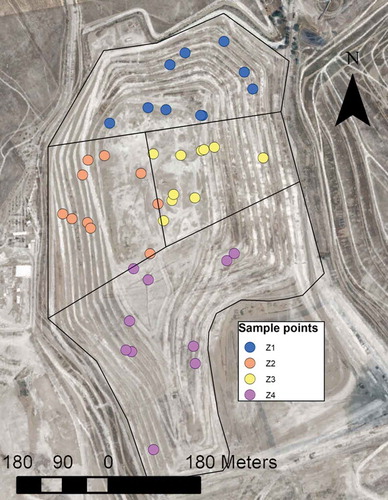
The flux chamber experimental method has been applied to a currently in-use Spanish landfill. This facility began to receive waste in 2000, and it is estimated that by the end of its life it will have received 22.7 million m³ of waste (Madrid 2017). Today, it is at about half capacity, with four cells already filled and sealed (labeled Z.1 to Z.4 in Figure 1b). The total emitting surface corresponding to these four cells is 335,000 m². The emitting surfaces of each cell are respectively 69,620, 72,082, 70,110, and 123,067 m², and the maximum filling heights in each cells are 39, 50, 47, and 40 m.

Figure 1. (a) Geographic location of the region of Madrid. (b) Landfill cell distribution.

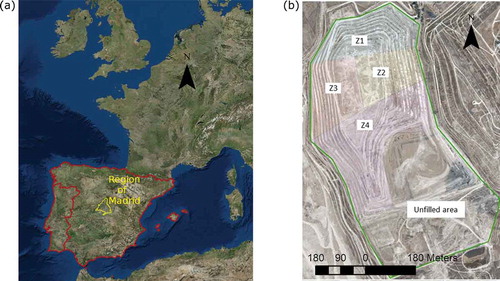
This landfill is integrated in a treatment center of solid urban wastes that includes several treatments such as separation, classification, composting, incineration, and leachate treatment by reverse osmosis. In addition, the recirculation of the leachate concentrate occurs. The cells are sealed with several layers of clay and sand, but these do not include high-density polyethylene sheets. A degassing system has been installed, but the extracted gas is flared and therefore its energy content is not recovered. Although the landfill began to receive waste in 2000, the degassing system did not start operating until 2004.

The landfill is located in the region of Madrid, in Spain, at the center of the Iberian Peninsula, as can be seen on Figure 1a. According to the Köppen-Geiger climate classification (Kottek et al. 2006), the climate in Madrid is type Csa, signifying generally warm temperatures and hot, dry summers. The quantitative emission measurement campaign was carried out in March 2016.

Methods

The method developed for the empirical analysis of methane emissions in landfills is based on the proposal by the UK EA in its publication Guidance on Monitoring Landfill Gas Surface Emissions (UK EA 2010). The method proposes a two-step approach. The first is a qualitative walkover survey to detect where emissions are being produced on the surface of the landfill. The second consists of a quantitative analysis of surface methane emissions at a selected number of points on the landfill surface.

The qualitative analysis serves as a first contact with the landfill. This procedure provides information on methane concentrations at each sampling point. The purpose of this study was therefore to identify the main surface emission points and check whether there were differences between different zones in the landfill. In this way, the study provided information that was valuable when planning the strategy for determining the sampling points for the quantitative analysis. The amount and distribution of the most significant emission sources were used as qualitative data to classify the landfill surface.

The process consists of a sweep walk of the landfill surface during which the concentration of methane at each point is measured. A Sensit portable methane detector (PMD; Valparaiso, Indiana) equipped with a probe to sample the air at ground level was used for this measurement. The analyzer measures methane concentrations with an accuracy of ±10% and a resolution of 1 ppm using infrared absorption spectroscopy in combination with an electronic narrow-band-pass filter. The PMD has a suction pump that drives the gas sample to be analyzed into the apparatus, facilitating a measurement with a response time of less than 3 sec. The Global Positioning System (GPS) and data-logging systems record the time, date, and location, in addition to the methane concentration.

The sample points for the second part of the survey, to quantitatively determine the emissions, are established using the information collected in the walkover survey. Surface emissions are then measured at each point using a flux box. This method has been widely used to measure soil fluxes of gases as well as to evaluate soil respiration. As recommended in Raco, Battaglini, and Lelli (2010) to reduce the influence of meteorological conditions, measurements of methane emissions were conducted on dry weather days and the measurement campaign was completed in three days.

The flux boxes are very simple devices, and for this work self-design ones (see Figure 2) based on UK EA recommendations have been used. The devices are constructed from 30-L polyethylene terephthalate (PET) containers with a footprint of 0.24 m² and a height of 20 cm. These dimensions create a balance between footprint surface, height, and volume. Further factors such as size and ease of use were also taken into account, and inexpensive; readily accessible materials were used to construct the devices.

Figure 2. (a) Diagram of flux box components. (b) Flux box during a landfill measurement.

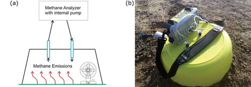
The devices have two openings: the gas mixture passes from the box chamber to the analyzer through one of the openings using the internal PMD pump. Once analyzed by the PMD, the sample is expelled and conducted back into the flux box through the second opening. The diagram in Figure 2 shows the components of the flux boxes used.

A Sensit PMD analyzer was used, as in the walkover survey, to measure the methane concentration inside the chamber. These analyzers allow the gas to be reinjected into the flux box after analysis, as it does not destroy the sample during the process (Bagnato et al. 2014; Elío et al. 2016). Measured in this way, the time of each analysis can be reduced from up to 1 hr to between 10 and 20 min with respect to measurements with no recirculation of analyzed gas. Plotting methane concentration versus time results in a line whose slope indicates the emission rate at that sampling point.

Statistical treatment

Total methane emissions have been estimated by applying the minimum variances unbiased estimator (MVUE) method (Koch and Link 1970; Parkin et al. 1988). This method provides better results for log-normal distributed data populations than the arithmetic mean (Elío et al. 2016). The method requires data independence to correctly calculate the confidence intervals. It is based on the Sichel function. This function has been calculated using R software (R Core Team 2016).

(1) ${\mathrm{\Psi }}_n\left(z\right)=1+\frac{z\left(n-1\right)}{n}+\frac{z^2{\left(n-1\right)}^3}{n^2\left(n+1\right)\cdot 2!}+\frac{z^3{\left(n-1\right)}^5}{n^3\left(n+1\right)\left(n+3\right)\cdot 3!}+\frac{z^4{\left(n-1\right)}^7}{n^4\left(n+1\right)\left(n+3\right)\left(n+5\right)\cdot 4!}+\dots$(1)

In this function, n is the number of sampling points and z is half of the variance as shown in eq 4.

(2) $u_i=\mathrm{l}\mathrm{n}\left(x_i\right)$(2)

(3) $\bar{u}=\frac{1}{n}\sum _i{u}_i$(3)

(4) $z=\frac{1}{2}{S}_u^2=\frac{1}{2\left(n-1\right)}\sum _i{\left(u_i-\bar{u}\right)}^2$(4)

where x_i in eq 2 is the methane emission in each point calculated from the slope of the concentration-versus-time plot.

Equations 5, 6, and 7 are used to estimate the mean (m) and the lower and upper limits (m_L and m_U) of the 95% (α = 0.05) confidence interval.

(5) $m=e^{\bar{u}}\cdot {\mathrm{\Psi }}_n\left(z\right)$(5)

(6) $m_{\mathrm{L}}=e^{U_L}\cdot {\mathrm{\Psi }}_n\left(z\right);U_L=\bar{u}-t_{\left(\frac{\alpha }{2},n-1\right)}\cdot \sqrt{\frac{S_u^2}{n}}$(6)

(7) $m_{\mathrm{U}}=e^{U_U}\cdot {\mathrm{\Psi }}_n\left(z\right);U_U=\bar{u}+t_{\left(\frac{\alpha }{2},n-1\right)}\cdot \sqrt{\frac{S_u^2}{n}}$(7)

where t_{(α/2, n-1)} is the t score from the t distribution corresponding to n − 1 degrees of freedom and α significance level. S_u² is the variance of the log-transformed above-zero emission.

The data have been divided into two populations for analysis. The first consists of the zero emission values (below the detection limit of the flux box), and the second comprises higher values. Total emissions are calculated as

(8) $E_{\mathrm{T}}=m\cdot P_{\ne 0}\cdot A$(8)

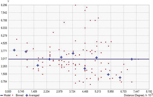
where m is the mean emission of the above-zero emission population calculated using eq 5, P_≠0 is the proportion of this population, and A is the total emitting surface. The data independence has been checked by plotting a variogram of the log-transformed above-zero emissions. The model parameters are optimized using the cross-validation tool of ArcGIS 10.3 software (ESRI, Redlands, California). The spherical model with nugget effect is the one that better describes the spatial variability of methane emissions. The resulting variogram describes the spatial variability as a horizontal line with sill and nugget equal so the independence of the data can be assumed, as can be seen in Figure 3.

Figure 3. Variogram of the log-transformed above-zero emissions. The horizontal line evidences data independence.

Mathematical models for landfill gas fugitive emissions

In recent years, a multitude of mathematical models have been developed to estimate fugitive methane emissions from landfills. In this study, the emissions from the previously described landfill have been calculated using two internationally recognized models: one proposed by the IPCC, the other by the EPA GHGRP. These are the most widely used models in the emission inventories in Europe and United States. These two models are very similar and are both based on determining organic matter decomposition using a first-order decay equation. In addition, a model developed by the company that manages this particular landfill has also been applied. This third model is also based on a first-order decay equation, but there are no details available about how methane production is calculated by this model. The results obtained using this model have been published and inventoried by Madrid City Council (MCC 2015).

For all three models, the total methane emission is calculated as

(9) $\begin{array}{rl}& \mathrm{C}{\mathrm{H}}_4\left(\mathrm{e}\mathrm{m}\mathrm{i}\mathrm{s}\mathrm{s}\mathrm{i}\mathrm{o}\mathrm{n}\right)=\mathrm{C}{\mathrm{H}}_4\left(\mathrm{p}\mathrm{r}\mathrm{o}\mathrm{d}\mathrm{u}\mathrm{c}\mathrm{t}\mathrm{i}\mathrm{o}\mathrm{n}\right)-\mathrm{C}{\mathrm{H}}_4\left(\mathrm{o}\mathrm{x}\mathrm{i}\mathrm{d}\mathrm{a}\mathrm{t}\mathrm{i}\mathrm{o}\mathrm{n}\right)\\ & -\mathrm{C}{\mathrm{H}}_4(\mathrm{c}\mathrm{o}\mathrm{l}\mathrm{l}\mathrm{e}\mathrm{c}\mathrm{t}\mathrm{i}\mathrm{o}\mathrm{n})\end{array}$(9)

Methane oxidation has been estimated in all cases as a 10% of that emitted. This is the default value proposed by the IPCC. On the other hand, the amount of methane extracted each year by the degassing system has been provided by the company that manages the facility. All the data on annual quantities of waste and its composition are presented in Table 1, whereas Table 2 presents the annual amount of methane collected.

Table 1. Input parameters of waste composition used in models for estimating methane emissions.

	Waste composition (1000 tons/yr)
Year	Paper	Textiles	Diapers	Food	Wood	Garden	Total waste
2000	149	18.3	14.2	92.7	56.5	24.8	667
2001	177	21.9	16.9	111	67.5	29.6	796
2002	172	21.2	16.4	107	65.4	28.7	772
2003	171	21.1	16.3	106	64.9	28.5	767
2004	182	22.4	17.3	113	69.2	30.4	816
2005	198	24.4	18.9	123	75.3	33.0	888
2006	204	25.1	19.4	127	77.5	34.0	915
2007	210	25.9	20.1	131	80.0	35.1	944
2008	199	24.6	19.0	124	75.8	33.3	895
2009	166	20.5	15.9	104	63.2	27.8	746
2010	156	19.3	14.9	97.6	59.5	26.2	703
2011	161	19.9	15.4	101	61.4	27.0	725
2012	160	19.8	15.3	100	61.0	26.8	721
2013	152	18.8	14.5	94.9	57.9	25.4	683
2014	155	19.2	14.8	96.9	59.1	25.9	697

Note. All data are shown in tons per year (1000 tons/yr) and provided by the company that manages the landfill.

Table 2. Tons of methane extracted by the degassing system each year reported by the company that manages the landfill.

Year	Methane extracted (tons/yr)
2000	0
2001	0
2002	0
2003	0
2004	0
2005	336.1
2006	709.2
2007	660.1
2008	668.0
2009	563.1
2010	562.3
2011	319.0
2012	429.1
2013	397.4
2014	411.7

The IPCC methodology can be implemented in three different tiers according the site-specific input data. In this study, tier 2 methodology has been applied, since the proposed default parameters for degradable organic carbon (DOC), fraction of DOC that can be anaerobically decomposed (DOCf), methane generation rate constant (k), methane correction factor (MCF), and fraction of methane in landfill gas (F) have been combined with specific data, provided by the company that manages the facilities, on the composition of the waste deposited in the landfill (IPCC 2006). The same data have been used to calculate the emissions using GHGRP methodology. The default parameters for each model are shown in Table 3.

Table 3. Default parameters for DOC, DOCf, k, MCF, and F for each landfill category.

	IPCC and GHGRP default parameters
Parameter (unit)	Paper	Textiles	Diapers	Food	Wood	Garden
DOC (tons carbon/tons waste)	0.4	0.24	0.24	0.15	0.43	0.2
DOCf (fraction)	0.5	0.5	0.5	0.5	0.5	0.5
k (L/yr)	0.04	0.04	0.05	0.06	0.02	0.05
MCF (fraction)	1	1	1	1	1	1
F (fraction by volume)	0.5	0.5	0.5	0.5	0.5	0.5

Note. These parameters are used to calculate methane emission with both IPCC and GHGRP models.

Results

Walkover survey

More than 20,000 points on the landfill surface were analyzed, and these are shown in Figure 4a. Table 4 gives a summary of the results obtained in the walkover survey. Figure 4b provides an interpolation of all these values. To generate this image, the weighted inverse distance interpolation (IDW) was applied using ArcGIS 10.3 software (Watson and Philip 1985).

Figure 4. (a) Walkover survey results. (b) Interpolation of walkover survey results using the weighted inverse distance method.

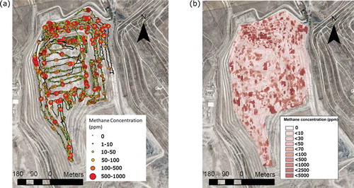
Table 4. Summary of walkover survey methane concentrations in ppm.

No.	Min.	Max.	Mean	Standard deviation
23,161	0	5.73 × 10^5	1.05 × 10^3	1.68 × 10^4

Note. No. = number of methane concentration measurements; Min., Max. = minimum and maximum values found.

Spatially, the distribution of the main sources of emissions that can be observed in Figure 4 shows slight variations in some of the side and slope areas. Even so, these variations are not clear enough to classify the landfill surface into several areas with different emissions, so the entire surface is taken as one for the quantitative analysis of the emissions. Despite this, the study of surface concentrations of methane is a valuable process in which the researcher can have a first contact with the surface of the landfill and check its status and the location of the main emission sources.

The total number of measurements taken was 40. This has been decided taking into account the limitations of time and access to the landfill facilities. In this way, 10 points were arbitrarily chosen in each of the cells into which the landfill is divided (Z.1 to Z.4), as illustrated in Figure 1. A random sampling method was chosen to determine these points, and their distribution is shown in Figure 5.

Figure 5. Locations of sampling points for the flux box campaign.

Experimental emissions

Once the sampling points had been chosen, the methane emissions at each one were measured. To do this, the flux box was placed on each of the correspondent points and sealed against the landfill surface to prevent gas escape. After this, the inlet and outlet ports of the chamber were opened, and the analyzer pump and data logging activated.

The 40 randomly selected points were measured in the winter of 2016 between 1 and 3 March 2016. The analysis time at each point was between 10 and 20 min. During this time, the analyzer recorded the methane concentration value inside the chamber every second. The plot of methane concentration versus time is linear, and the emissions can be calculated from the slope (dC/dt). The mathematical relationships between the slope and the emissions expressed in L/m²·hr and in mg/m²·hr are shown in eqs 10 and 11, respectively. Table 5 presents the emissions obtained for each sampling point (mg/m²·hr) in the four cells.

(10) $E=\frac{V\left(\mathrm{d}C/\mathrm{d}t\right)}{a}\times 0.001\times 3600$(10)

Table 5. Methane emissions (mg/m²·hr) at each sampling point.

Point	Emission	Point	Emission	Point	Emission	Point	Emission
Z1.1	38.9	Z2.1	0	Z3.1	19.6	Z4.1	278.1
Z1.2	141.0	Z2.2	0	Z3.2	0	Z4.2	209.9
Z1.3	748.8	Z2.3	30.0	Z3.3	0	Z4.3	221.0
Z1.4	0	Z2.4	—	Z3.4	276.7	Z4.4	1350.0
Z1.5	0	Z2.5	0	Z3.5	0	Z4.5	194.9
Z1.6	0	Z2.6	8526.1	Z3.6	107.9	Z4.6	0
Z1.7	699.0	Z2.7	18.8	Z3.7	254.7	Z4.7	1079.6
Z1.8	55.0	Z2.8	8.7	Z3.8	143.0	Z4.8	6229.7
Z1.9	7.8	Z2.9	40.4	Z3.9	48278.8	Z4.9	2916.1
Z1.10	1189.0	Z2.10	0	Z3.10	2228.4	Z4.10	0

where E is the level emissions (L/m²·hr); dC/dt is the change in concentration with time (ppm/sec); V is the flux box volume (m³); and a is the flux box footprint (m²).

(11) $E^{\prime }=E\times \frac{P}{0.082\cdot T}\times 1600$(11)

where E′ is the level of emission (mg/m²·hr); P is the atmospheric pressure (atm); and T is the temperature inside flux box (K).

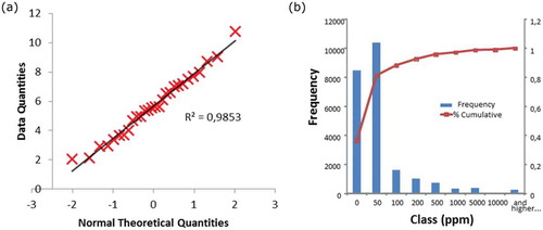
The log-normal distribution of the nonzero data population has been checked using a Q-Q diagram. As can be seen in Figure 6, the data are suitably fitted to this distribution.

Figure 6. (a) Q-Q diagram for nonzero data population. (b) Histogram of frequencies and cumulative frequency graph for walkover survey results.

Applying the statistical approach previously described, the average emission of the landfill surface is 74.9 g·m⁻²·day⁻¹, with 27.8 and 202.1 74.9 g·m⁻²·day⁻¹ as the lower and upper limits of the 95% confidence interval, respectively. These values are within the ranges reported in other landfill studies; for example, Capaccioni et al. recorded levels of between 0.30 and 170.40 g·m⁻²·day⁻¹ (Capaccioni et al. 2011), and these are in the same order of magnitude as those reported by Borjesson, Danielsson, and Svensson (2000) of between 8.37 and 42.6 g·m⁻²·day⁻¹.

Total emission for the landfill, with an emitting surface of 334,879 m², is 9.16 × 10³ ton/yr; the upper and lower limits of the 95% confidence interval calculated are 3.40 × 10³ and 24.7 × 10³ ton/yr.

Modeled emissions

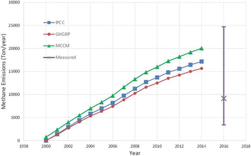
Figure 7 shows the methane emissions calculated from 2000 to 2014 using the previously mentioned models, and the data are shown in Tables 1–2. The result of the model proposed by the company that manages the landfill is referred to in the plot as MCCM (Madrid City Council Model). Additionally, the measured emission data and their confidence intervals are represented for the year 2016.

Figure 7. Comparison between modeled and measured annual emissions.

Discussion

As can be seen in Figure 6b, about 80% of the sampling points have low concentrations (between 0 and 50 ppm). This means that approximately 20% of the points analyzed in this survey are above 50 ppm; in other words, they could be considered significant methane emission sources. The distribution of these main emission points over the landfill surface is fairly random, as shown in Figure 4. As previously discussed, there are not large differences between emissions on the upper surface of the landfill and its side slopes or other areas. For this reason, the sampling points for the flux box emission measurement campaign were chosen randomly, without taking into account the slight differences founded across the landfill.

As reported in Xu et al. (2014), there is a strong dependence of methane emissions on changes in barometric pressure. This phenomenon, called barometric pumping, occurs when the emissions decrease as a result of an increase in pressure and, on the contrary, increase when there is a sudden drop in pressure. This effect is more pronounced when the variation in pressure occurs in a short time.

During the three days in which the measurement campaign has been developed, atmospheric conditions have been far from extreme values, as can be seen in Table 6. The temperatures were normal for the season, and there have been no abrupt changes in atmospheric pressure during the hours at which the measurements were made between 10 a.m. and 2 p.m. on each day, so it can be assumed that the effect of atmospheric conditions on the measurements is minimal (Di Bella, Di Trapani, and Viviani 2011).

Table 6. Meteorological conditions during the measurement campaign.

	Meteorological parameters during measurement campaign
Campaign	Temperature (°C)	Humidity (%)	Pressure (mbar)	Wind speed (m/sec)	Wind direction (°)
1 March 2016	10.8	46.5	950	3.12	31
2 March 2016	10.9	53.8	947	1.26	351
3 March 2016	11.1	53.8	944	1.04	146

Note. The values shown are average values for the hours during which the measurements were taken: from 10:00 a.m. to 2:00 p.m. each day.

In this campaign, methane emission point values ranging from zero to almost 50,000 mg/m²·hr were found. This large variability in emission values, a consequence of the heterogeneity of the landfill surface, causes great uncertainty when determining an average emission value for the landfill. This uncertainty is reflected in the confidence interval for the total annual emission. Other authors (Borjesson, Danielsson, and Svensson 2000) have also remarked upon this important variability in the results and the difficulty of estimating annual emissions from point emission measurement in a single campaign, as a few points are responsible of the total emission of the landfill. On the other hand, making this estimate is necessary in order to be able to compare the experimental results with those obtained using models. Although the uncertainty in the annual emissions calculated is large, this comparison can give valuable information when deciding whether the results obtained with the models are adjusted to reality or not.

The emissions calculated using the three proposed models vary between 15,000 and 20,000 tons for the year 2014. The values calculated by the models are between 1.7 and 2.2 times higher than the annual average calculated from the measurements but below the 95% upper confidence limit. This point to a slight overestimation of the emissions by the three models, which is in agreement with other studies, such as de laCruz et al. (2016) or Vu, Ng, and Richter (2017). The first of these studies has reported greater discrepancies between the results obtained with the models and those measured. In this study, the models give values between 4 and 31 times greater than the experimental data.

In any case, the comparison between the emissions determined using a short-term measurement case study and the models should be treated with caution. There is a great uncertainty in the calculated values due to two factors: the great variability of emissions that can be found in the surface of the landfill and the estimation of the annual emissions from data taken in just three days. There are two ways to improve the experimental results of the proposed method. First of all, it is recommended that a series of periodic campaigns be conducted to reflect the temporal variability of emissions and improve the representativeness of the results obtained. The second way to improve the results could be to take a greater number of measurements in each campaign to minimize spatial uncertainty.

Summary

Although the confidence intervals in the results are wide, the method chosen to measure emissions can provide valuable information to assess the emissions estimated by the models. The average value obtained with measurements approximates to those provided by the three models, and even though the figures from these are all higher than the results of the experimental technique, they are all within the upper confidence interval. As previously mentioned, an increase in the number of measurement points and a greater number of measurement campaigns over time could lead to more accurate results to confirm whether the models are actually overestimating methane emissions.

However, although the mean result obtained is in accordance with the values from the models, the associated confidence interval is very large. This reflects the complexity of the landfill and the heterogeneity of its large surface area. Nevertheless, and despite the limited number of measurements taken, this high level of uncertainty is similar to that reported by other authors (Borjesson, Danielsson, and Svensson 2000; Capaccioni et al. 2011; Di Trapani, Di Bella, and Viviani 2013).

As for the models evaluated, all three give very similar results, as they are all based on quite similar equations and the same parameters are used. The value provided by the GHGRP model is slightly closer to the average value obtained experimentally than those provided by the other models. Even so, a more accurate estimate of the surface oxidation of methane could adjust the values predicted by the models to the experimental ones. Several studies (Chanton, Powelson, and Green 2009; Spokas, Bogner, and Chanton 2011) have concluded that this oxidation is underestimated by a value of 10% and therefore the emissions calculated with the models are overestimated.

Additional information

Funding

This study was developed in the scope of the “Optimización de la gestión de residuos municipales” project (CTQ 2013-48280-C3-2R), funded by the Spanish Ministry of Economy and Competitiveness.

Notes on contributors

Carlos Sánchez

Carlos Sánchez is a Ph.D. candidate in the Department of Chemical and Environmental Engineering, Technical University of Madrid (UPM).

Maria del Mar de la Fuente

Maria del Mar de la Fuente, Adolfo Narros, and Isabel del Peso are lecturers in the Department of Chemical and Environmental Engineering, Technical University of Madrid (UPM).

Encarnación Rodríguez

Encarnación Rodríguez is a professor in the Department of Chemical and Environmental Engineering, Technical University of Madrid (UPM).

References

- Abichou, T., J. Clark, D. Goldsmith, M. A. Barlaz, and N. Swan. 2010. Uncertainties associated with the use of optical remote sensing technique to estimate surface emissions in landfill applications. J. Air Waste Manage. Assoc. 60 (4):460–70. doi:10.3155/1047-3289.60.4.460.
- Babilotte, A., T. Lagier, E. Fiani, and V. Taramini. 2010. Fugitive methane emissions from landfills: Field comparison of five methods on a French landfill. J. Environ. Eng. 136 (8):777–84. doi:10.1061/(ASCE)EE.1943-7870.0000260.
- Bagnato, E., M. Barra, C. Cardellini, G. Chiodini, F. Parello, and M. Sprovieri. 2014. First combined flux chamber survey of mercury and CO2 emissions from soil diffuse degassing at Solfatara of Pozzuoli Crater, Campi Flegrei (Italy): Mapping and quantification of gas release. J. Volcanol. Geotherm. Res. 289:26–40. doi:10.1016/j.jvolgeores.2014.10.017.
- Battaglini, R., B. Raco, and A. Scozzari. 2013. Effective monitoring of landfills: Flux measurements and thermography enhance efficiency and reduce environmental impact. J. Geophys. Eng. 10 (6):064002. doi:10.1088/1742-2132/10/6/064002.
- Bella, G., D. Di Trapani, and G. Viviani. 2011. Evaluation of methane emissions from Palermo municipal landfill: Comparison between field measurements and models. Waste Manag. 31 (8):1820. doi:10.1016/j.wasman.2011.03.013.
- Borjesson, G., A. Danielsson, and B. H. Svensson. 2000. Methane fluxes from a Swedish landfill determined by geostatistical treatment of static chamber measurements. Environ. Sci. Technol. 34 (18):4044–50. doi:10.1021/es991350s.
- Campuzano, R., and S. Gonzalez-Martinez. 2016. Characteristics of the organic fraction of municipal solid waste and methane production: A review. Waste Manag. 54:3–12. doi:10.1016/j.wasman.2016.05.016.
- Capaccioni, B., C. Caramiello, F. Tatàno, and A. Viscione. 2011. Effects of a temporary HDPE cover on landfill gas emissions: Multiyear evaluation with the static chamber approach at an Italian landfill. Waste Manag. 31 (5):956–65. doi:10.1016/j.wasman.2010.10.004.
- Chanton, J. P., D. K. Powelson, and R. B. Green. 2009. Methane oxidation in landfill cover soils, is a 10% default value reasonable? J. Environ. Qual. 38 (2):654–63. doi:10.2134/jeq2008.0221.
- de laCruz, F. B., R. B. Green, G. R. Hater, J. P. Chanton, E. D. Thoma, T. A. Harvey, and M. A. Barlaz. 2016. Comparison of field measurements to methane emissions models at a new landfill. Environ. Sci. Technol. 50 (17):9432–41. doi:10.1021/acs.est.6b00415.
- Di Trapani, D., G. Di Bella, and G. Viviani. 2013. Uncontrolled methane emissions from a MSW landfill surface: Influence of landfill features and side slopes. Waste Manag. 33 (10):2108–15. doi:10.1016/j.wasman.2013.01.032.
- Elío, J., M. F. Ortega, B. Nisi, L. F. Mazadiego, O. Vaselli, J. Caballero, and E. Chacón. 2016. A multi-statistical approach for estimating the total output of CO2 from diffuse soil degassing by the accumulation chamber method. Int. J. Greenhouse Gas Control 47:351–63. doi:10.1016/j.ijggc.2016.02.012.
- Gonzalez-Valencia, R., F. Magana-Rodriguez, E. Maldonado, J. Salinas, and F. Thalasso. 2015. Detection of hotspots and rapid determination of methane emissions from landfills via a ground-surface method. Environ. Monit. Assess. 187 (1):4083. doi:10.1007/s10661-014-4083-0.
- Intergovernmental Panel on Climate Change (IPCC). 2006. 2016 Ipcc guidelines for national greenhouse gas inventories. In: Eggleston, H.S., Buendia, L., Miwa, K., Ngara, T., Tanabe, K. (Eds.), Prepared by the National Greenhouse Gas Inventories Programme. http://www.ipcc-nggip.iges.or.jp/public/2006gl/spanish/
- Kamalan, H., M. Sabour, and N. Shariatmadari. 2011. A review on available landfill gas models. J. Environ. Sci. Technol. 4 (2):79–92. doi:10.3923/jest.2011.79.92.
- Koch, G. S., and R. F. Link. 1970. Statistical analysis of geological data, Vol. 1, 201–53. New York: Wiley.
- Kormi, T., S. Mhadhebi, N. B. H. Ali, T. Abichou, and R. Green. 2018. Estimation of fugitive landfill methane emissions using surface emission monitoring and Genetic Algorithms optimization. Waste Manag. 72:313–28. doi:10.1016/j.wasman.2016.11.024.
- Kottek, M., J. Grieser, C. Beck, B. Rudolf, and F. Rubel. 2006. World map of the Koppen-Geiger climate classification updated. Meteorol. Z. 15 (3):259–63. doi:10.1127/0941-2948/2006/0130.
- Madrid, E. 2017. Centro Las Dehesas: Vertedero controlado de rechazos y RU no aprovechables - Ayuntamiento de Madrid. http://www.madrid.es/portales/munimadrid/es/Inicio/El-Ayuntamiento/Medio-ambiente/Residuos-y-limpieza-urbana/Parque-Tecnologico-de-Valdemingomez/Informacion-relativa-al-Parque/Centros-de-Tratamiento/Centro-de-Las-Dehesas/Centro-Las-Dehesas-Vertedero-controlado-de-rechazos-y-RU-no-aprovechables?vgnextfmt=detNavegacion&vgnextoid=8b748a6971618210VgnVCM2000000c205a0aRCRD&vgnextchannel=5cb9dc186a865210VgnVCM1000000b205a0aRCRD
- Majdinasab, A., Z. Zhang, and Q. Yuan. 2017. Modelling of landfill gas generation: A review. Rev. Environ. Sci. Biotechnol. 16 (2):361–80. doi:10.1007/s11157-017-9425-2.
- MAPAMA (Ministerio de agricultura y Pesca, Alimentación y Medio Ambiente). 2014. RESIDUOS DE COMPETENCIA MUNICIPAL. Dirección General de Calidad y Evaluación Ambiental y Medio Natural. https://www.miteco.gob.es/va/calidad-y-evaluacion-ambiental/publicaciones/memoriaanualdegeneracionygestionderesiduosresiduosdecompetenc_tcm39-432352.pdf.
- Maurice, C., and A. Lagerkvist. 2003. LFG emission measurements in cold climatic conditions: Seasonal variations and methane emissions mitigation. Cold Reg. Sci. Technol. 36:37–46. doi:10.1016/s0165-232x(02)00094-0.
- MCC (2015). Air pollutant emissions inventory of the municipality of Madrid 2013. Deputy Directorate for Energy and Climate Change. Madrid City Council. http://www.madrid.es/UnidadesDescentralizadas/Sostenibilidad/EspeInf/EnergiayCC/04CambioClimatico/4aInventario/Ficheros/GHGemissions2014.pdf
- Mønster, J., J. Samuelsson, P. Kjeldsen, and C. Scheutz. 2015. Quantification of methane emissions from 15 Danish landfills using the mobile tracer dispersion method. Waste Manag. 35:177–86. doi:10.1016/j.wasman.2014.09.006.
- Myhre, G., B. H. Samset, M. Schulz, Y. Balkanski, S. Bauer, T. K. Berntsen, H. Bian, N. Bellouin, M. Chin, T. Diehl, R. C. Easter, J. Feichter, S. J. Ghan, D. Hauglustaine, T. Iversen, S. Kinne, A. Kirkevåg, J.-F. Lamarque, G. Lin, X. Liu, M. T. Lund, and G. L. C. Zhou. 2013. Radiative forcing of the direct aerosol effect from AeroCom phase II simulations. Atmos. Chem. Phys. 13:1853–77. doi:10.5194/acp-13-1853-2013.
- Parkin, T. B., J. J. Meisinger, J. L. Starr, S. T. Chester, and J. A. Robinson. 1988. Evaluation of statistical estimation methods for lognormally distributed variables. Soil Sci. Soc. Am. J. 52 (2):323–29. doi:10.2136/sssaj1988.03615995005200020004x.
- R Core Team. 2016. R: A language and environment for statistical computing. Vienna, Austria: R Foundation for Statistical Computing. Accessed 2016 http://www.R-project.org/.
- Raco, B., R. Battaglini, and M. Lelli. 2010. Gas emission into the atmosphere from controlled landfills: An example from legoli landfill (Tuscany, Italy). Environ. Sci. Pollut. Res. 17 (6):1197–206. doi:10.1007/s11356-010-0294-2.
- Solomon, S., D. Qin, M. Manning, Z. Chen, M. Marquis, K. B. Averyt, M. Tignor, and H. L. Miller. 2007. Climate change 2007: The physical science basis. Contribution of Working Group I to the Fourth Assessment Report of the Intergovernmental Panel on Climate Change. Cambridge University Press, Cambridge, United Kingdom and New York, NY, USA, 996 pp. http://www.ipcc.ch/publications_and_data/publications_ipcc_fourth_assessment_report_wg1_report_the_physical_science_basis.htm.
- Spokas, K., J. Bogner, and J. Chanton. 2011. A process‐based inventory model for landfill CH4 emissions inclusive of seasonal soil microclimate and CH4 oxidation. J. Geophys. Res. 116:G04017. doi:10.1029/2011JG001741.
- UK EA. 2010. Guidance on monitoring landfill gas surface emissions. Doc LFTGN07, Environment Agency, Bristol.
- Vu, H. L., K. T. W. Ng, and A. Richter. 2017. Optimization of first order decay gas generation model parameters for landfills located in cold semi-arid climates. Waste Manag. 69:315–24. doi:10.1016/j.wasman.2017.08.028.
- Watson, D. F., and G. M. Philip. 1985. A refinement of inverse distance weighted interpolation. Geoprocessing 2:315–27.
- Wong, C. L. Y., and J. Ramkellawan. 2013. Calibration of a fugitive emission rate measurement of an area source. J. Air Waste Manag. Assoc. 63 (11):1324–34. doi:10.1080/10962247.2013.823895.
- Xu, L. K., X. M. Lin, J. Amen, K. Welding, and D. McDermitt. 2014. Impact of changes in barometric pressure on landfill methane emission. Global Biogeochem. Cycles. 28 (7):679. doi:10.1002/2013gb004571.