Development of the typical driving cycle for buses in Hanoi, Vietnam

ABSTRACT

This paper develops a typical driving cycle for buses in Hanoi that does not require the deconstruction of the natural driving patterns. Real velocity–time data were collected along 15 routes in the inner city. The raw velocity–time series were preprocessed to remove errors, and smooth and denoise the data. These data, then, were tested for stationary behavior before being used in the construction of the driving cycle based on Markov chain theory. The 14 representative parameters of the driving cycle, including vehicle-specific power, which were extracted from 33 driving cycle parameters using the hierarchical agglomerative clustering method, were used to integrate the features of realistic driving patterns into the typical driving cycle. The conformity of the developed driving cycle with the real-world driving data was evaluated by the speed–acceleration frequency distribution (SAFD). A typical driving cycle for buses in Hanoi with a SAFD of 13.2% was developed. This is the first driving cycle developed for buses in Vietnam.

Implications: A typical driving cycle was developed for the first time for buses in Hanoi. With the deviation in speed-acceleration frequency distribution (SAFD) reaching to 13.2%, the developed driving cycle reflects well the overall real-world driving data in the city. This driving cycle, therefore, can be applied for the development of the country-specific emission factors and emission inventories for buses which are a very good tool as well as useful information for integrated air quality management in Hanoi.

Introduction

Hanoi is undergoing a rapid modernization process. It has been continuously trying to develop an urban transport system to meet its explosive growth rate for many years. In this context, the bus is considered to be a potentially significant contributor to the public transport system of Hanoi. Since 2001, the city has stepped up the development of its bus system through the improvement of its fleet and the expansion of the route network.The Hanoi bus system has been considerably developed in recent years, with the network now covering all 30 districts of the city. The number of bus routes, the fleet and the number of passengers have been increased 3 times (from 31 to 92 routes), 4.2 times (from 334 to 1404 vehicles) and 28.7 times, respectively (Ministry of Transport, 2018). However, due to a poor transportation infrastructure combined with a high vehicle density and frequent traffic jams, the average bus speed is only about 15 kph (Transerco, 2018). Aditional problems include: poor maintenance, bad fuel quality and old vehicles that do not meet emission standards and thus are a significant emitter of air pollutants including PM, NOx, CO and SO₂, affecting the air quality of the city. As a result, levels of PM₁₀ and PM_2.5 in the urban areas of Hanoi exceed Vietnam’s ambient air quality standards on more than 20% of the total days of the year (MONRE, 2016).

In Vietnam, the emission inventories for the transport sector mainly use emission factors adopted from other countries and organizations such as the World Health Organization, and Intergovernmental Panel on Climate Change. Thus, they do not wholly reflect the emission characteristics of vehicles in Vietnam, which significantly depend on local driving patterns. The use of country-specific emission factors (CSEFs) instead of values from other countries can reduce the level of uncertainty in national emission inventories (LEAD, 2013). Hence, developing the CSEF is a very important prerequisite before any emission inventory design and implementation can take place. Emission factors are normally obtained from emission data monitored in laboratories or under actual conditions. According to Franco et al. (2013), the method of emission measurement under controlled conditions in laboratories (dynamometer tests) is ideal for the development of the CSEF when the local driving cycles are constructed. A driving cycle is defined as a profile of velocity versus time of a vehicle operating under a stated circumstance that reflects real-world driving characteristics. The driving cycle is developed from data collected by driving the tested vehicle on the actual road network. The driving cycle provides foundational data for the design of vehicles and plays a critical role in the monitoring of emissions. The realistic driving characteristics (reflected in the driving cycle) depend on local conditions, and can be different from one region to another (Tong et al., 2011). A previous study performed by the current authors showed that the real-world driving characteristics in Vietnam are very different from those in Europe (Nguyen and Nghiem, 2017). Therefore, the application of emission factors from other countries, including the European Union, to the situation in Vietnam would result in an increase in the level of uncertainty in the country’s emission inventories. However, studies on the construction of a local driving cycle for road vehicles in Vietnam are still scarce. To the best of our knowledge, no such data for road vehicles in Vietnam are available in the open or published literature, except for a few studies on motorcycles and light-duty vehicles such as Tong et al. (2011) and Le et al. (2012).

Most studies in the literature have used microtrips to produce a driving cycle based on different selection and combination methods of microtrips, in which each microtrip is a trip segment between consecutive vehicle stops (Amirjamshidi and Roorda, 2015; Perhinschi et al., 2011). However, the frequency distribution of operation modes of the driving cycle is not fully captured in this approach when the vehicle emission rate depends strongly on the distribution of operation modes. Therefore, construction methods for a driving cycle that are based on microtrips are not robust and cannot fully reflect the stochastic nature of the obtained data (Lin and Niemeier, 2003).

To address the limitations of previous driving cycle construction methods, in 2002, Lin and Niemeier initiated using the Markov chain approach to construct the driving cycle (Lin, 2002; Lin and Niemeier, 2002). Since then, this approach has been applied to the construction of driving cycles by many researchers, for example, Bishop, Axon, and McCulloch (2012), Brady and O’Mahony (2013), Ashtari, Bibeau, and Shahidinejad (2014). The concept of a Markov chain is described in Gubner (2006). A series of random variables X₁, X₂, X₃,… is considered to have the Markov property provided that:

(1) $\begin{array}{c}P(X_{n+1}=x_{n+1}|X_1=x_1,X_2=x_2,...,X_n=x_n)\\ =P(X_{n+1}=x_{x+1}|X_n=x_n)\end{array}$(1)

The set of random variables X_n is called the state space of the chain. The conditional probabilities p_ij: = P(X_n+1 = j|X_n = i) are called transition probabilities. Note that the sum of all probabilities leaving a state must be unity:

(2) $\sum _j{p}_{\mathrm{i}\mathrm{j}}=\sum _{j}P(X_{n+1}=j|X_n=i)=1$(2)

In Lin’s thesis (Lin, 2002), driving patterns such as acceleration, deceleration, cruising, idling are defined as the states in a Markov process. In more recent studies, the speed and acceleration of the vehicle have been proposed as states for the Markov chain to acquire the characteristics of real-world driving (Bishop, Axon, and McCulloch, 2012; Lee and Filipi, 2011; Shi et al., 2016). The real-world velocity and acceleration data series with a 1-sec step were determined to have Markov property (Shi et al., 2016), therefore, the Markov process is a suitable approach to use in the development of a driving cycle.

In the construction of a driving cycle, the characteristic parameters of the driving cycle are always used as basis to capture the features of realistic driving patterns and are introduced into the typical driving cycle. They are also used as assessment criteria to choose a typical driving cycle. However, in almost all previous studies, the selected parameters mainly present the driving characteristics, but do not fully reflect emission characteristics (Lai et al., 2013). Jimenez-Palacios (1999) introduced a new parameter, vehicle-specific power (VSP), to understand the emission of motor vehicles. The advantage of VSP is that its distribution closely reflects both the driving and the emission characteristics (Dai, Niemeier, and Eisinger, 2008; Duarte, Gonçalves, and Farias, 2016; EPA, 2010). Therefore, VSP is a useful parameter for emission studies (Haibo, Frey, and Nagui, 2008; Hallmark and Qiu, 2012; Guohua, Lei, and Zhao, 2012; Lai et al., 2013; Qi et al., 2016; and so on). In the study of Dai, Niemeier, and Eisinger (2008), the average speed and VSP bin distribution were used to classify driving patterns before cycle development based on a modal approach in which the driving process is treated as a random process of Markov chain. Lai et al. (2013) used VSP as an assessment criterion for selecting representative microtrips; the selected microtrips were then used to construct the final driving cycle by combining them in ascending order of the root mean squared error of each single microtrip until the predetermined cycle duration was achieved. Obviously, in these studies, the typical driving cycles are still generated from microtrips or snippets and VSP is only used as criterion to segment the speed versus time profile into microtrips or to classify driving patterns. However, as previously mentioned, this approach cannot fully capture real-world driving characteristics. Therefore, in this study, VSP was used as the criterion for the assessment and selection of a typical driving cycle that was developed based on Markov chain theory, and in which vehicle velocity and acceleration were used as states. This approach to the construction of a driving cycle is similar to that used in the studies of Lee and Filipi (2011) and Torp and Önnegren (2013), but emission-related variables were added that were used as the criterion of conformity assessment of the candidate cycles with the real-world driving data.

Material and methods

There are three critical components in the construction of a driving cycle, these are route selection, data collection and cycle construction (Tong and Hung, 2010). These components are briefly introduced in this section. In addition, the methods of data preprocessing and the evaluation of candidate driving cycles are also briefly presented.

Route selection

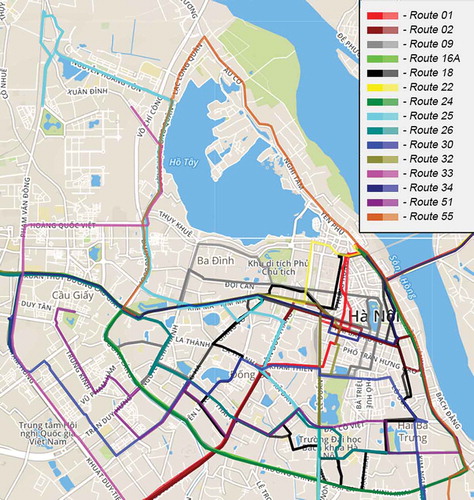
Routes were selected in a manner to represent the typical driving patterns observed in the study area. The routes were also selected based on the judgment of researchers, such as relying on home-to-work trips, the difference in population density and road classifications. These factors need to be carefully taken into account in the selection of routes for study (Tong and Hung, 2010). With this approach, 15 Hanoi urban routes covering all three route types were selected as presented in Table 1 and Figure 1. Figure 1 was created using GeoJson (2018), the open source software with permission from the Massachusetts Institute of Technology. There are three bus routes (No. 01, 22 and 34) that have their final destination point in a suburban area, hence, trip segments that extend beyond the inner city need be trimmed in order to conform with the objectives of this study, these segments are not included in Figure 1.

Table 1. The summary information of the 15 bus routes used in this study.

		Information
Route	Route type	Average length^(*) (km)	Average velocity (kph)	No. of vehicles per route
09	Circular	19.8	15	18
18		19.2	14	12
01	Radial	21.7	17	19
02		17.2	16	32
22		14.2	15	20
32		18.1	16	33
16	Straight	15.0	16	17
24		15.1	14	14
25		28.2	18	21
26		17.9	15	29
30		16.0	15	19
34		17.9	16	19
33		19.8	17	12
51		17.0	17	11
55		19.1	19	8

Source: Bus-WebGPS (2018)

Notes. ^(*) The average length of both directions on each bus route as these directions are not the same roads.

Figure 1. Map of bus routes for data collection.

Collection of real-world driving data

There are three main approaches to the collection of real-world driving data: the chase car method, on-board measurement, and the use of a Global positioning system (GPS) technique (Niemeier, Limanond, and Jennifer, 1999). Of these approches, GPS devices have been demonstrated to be most useful for collecting real-world driving data, as a vehicle’s speed and position can be continuously captured by this technology (Niemeier, Limanond, and Jennifer, 1999; Tong and Hung, 2010). The benefits of the GPS technique are that GPS devices are easy to instal and they are a cost-effective tool. Therefore, it is a widely utilized technique for gathering real-world driving data for vehicles (Duran and Earleywine, 2012).

Hence, a GPS (Garmin etrex vista HCx), with the frequency resolution of 1Hz, was used in this study to collect travel data from buses on 15 selected routes, with one vehicle being selected randomly per route. The information obtained on these 15 selected routes is presented in Table 1. On each bus route, real-world driving data were recorded continuosly, from the starting point at around 6.00 a.m. to the finishing point at around 8.00 p.m., on weekdays as well as at weekends, during the period of September 2015 to September 2016. Data were collected in every second to avoid losing information and to make sure that the real-world driving data has the Markov property (Shi et al., 2016).

GPS data preprocessing

In order to be used for the study, collected GPS data have to be processed to remove errors, which are normally caused by a sudden loss of signal, data spiking, white noise in the signal, and zero-speed drift. These errors significantly affect the quality of data, and therefore, restrict the efficiency of the process to create the driving cycle (Duran and Earleywine, 2012). Thus, the good preprocessing procedure is required to ensure that the errors are minimized, but the integrity of the data is kept. Based on the study of Duran and Earleywine (2012), a filtration process for improving the quality of GPS data was proposed including the following steps:

1. Initialize the trip segments

2. Remove duplicate records or negative time period

3. Replace outlying speed values

4. Remove zero-speed signal drift

5. Replace false zero-speed records

6. Amend gaps in data

7. Repair outlying acceleration values

8. Denoise and smooth final signals

In this paper, only new features, which are different from the study of Duran and Earleywine (2012), are mentioned. A bus trip segment, which is used to develop the driving cycle, is assumed to be a movement between the start and end points of one bus on each route. Therefore, using the driving data collection method as discussed above, collected GPS data must be split into trip segments, in which each segment must start and end with zero-speed values. This is an initial step of the filtration process. From steps 3–7, the detection of erroneous data points was carried out similarly to the study of Duran and Earleywine (2012), but repaired in a different way. In this study, the missing data estimation algorithm, which was developed by Selesnick (2013), was used. According to this approach, erroneous data points are deleted to create data gaps, and after that the algorithm of Selesnick (2013) is used to estimate the values of these data points. In step 8, a Kalman filter is used to denoise and smooth final signals, rather than using the Savitzky–Golay filter as done in the study of Duran and Earleywine (2012). The Kalman filter is believed to be better than many other smoothing techniques (Jun, Guensler, and Ogle, 2006; Lavagnini, Pastore, and Magno, 1990). This is a useful tool for reducing the impact of noise signals while retaining the whole of the driving data profile. The Kalman filter smooths data points and denoises data by recursively modifying error values. The values of the measured noise (R) and the process noise (Q) are required for the Kalman filter. The rate of data capture in this study is 1Hz, similar to the study of Jun, Guensler, and Ogle (2006), thus, Q = 0.25 and R = 0.25 were chosen. In this case, the Kalman filter is called the modified Kalman filter.

Data processing

All cleaned GPS data went through a processing stage as follows.

Calculation of acceleration and average velocity

The acceleration and the average velocity are calculated in the same time interval, between each two points with the time step of 1 sec according to Torp and Önnegren (2013).

Extraction of driving cycle parameters

This is a very important step in the data processing. The values extracted here are later used for representative parameter analysis and conformity assessment. As previously mentioned, according to Lai et al. (2013), the selected parameters represent the driving characteristics, but do not fully reflect emission characteristics. Therefore, similar to several other studies (Dai, Niemeier, and Eisinger, 2008; Lai et al., 2013), in this study, a VSP parameter was added, due to its strong correlation with emission characteristics. The driving cycle parameters were calculated based on Jimenez et al. (1999), Barlow et al. (2009) and Ashtari, Bibeau, and Shahidinejad (2014). These parameters are presented in Table 2. The definitions of these parameters, which are shown in the Supplemental Material, are applied to a velocity profile consisting of n data rows of time t_i in second, and speed v_i in kph, with 1 ≤ i ≤ n.

Table 2. The parameters of driving cycle.

Group	Parameter	Units
Distance related	Total distance	km
Time related	Total time	sec
	Acceleration time	sec
	Deceleration time	sec
	Cruising time	sec
	Creeping time	sec
	Idle time (speed = 0)	sec
	Time proportion of acceleration mode	%
	Time proportion of deceleration mode	%
	Time proportion of cruising mode	%
	Time proportion of creeping mode	%
	Time proportion of idling mode	%
Speed related	Average trip speed	kph
	Average driving speed	kph
	Standard deviation of speed	kph
	Maximum speed	kph
	95th percentile of speed	kph
Acceleration related	Maximum acceleration	m.sec^−2
	Minimum acceleration	m.sec^−2
	Acceleration average	m.sec^−2
	Average positive acceleration	m.sec^−2
	Average negative acceleration	m.sec^−2
	Standard deviation of acceleration	m.sec^−2
	95th percentile of positive acceleration	m.sec^−2
	95th percentile of negative acceleration	m.sec^−2
Stop related	Number of stops	-
	Number of stops per km	/km
Dynamics related	Positive kinetic energy (PKE)	m.sec^−2
	Root mean square of acceletration (RMSA)	m.sec^−2
	Vehicle specific power (VSP): +Maximum VSP +Minimum VSP +Average positive VSP +Average positive VSP	W.kg^−1

Determination of representative driving cycle variables

The processed GPS data were then used to develop a typical driving cycle for buses in Hanoi. However, first, the characteristic parameters (known as target or assessment ones) of a driving cycle must be determined. These parameters are the basis to capture the features of realistic driving patterns and bring them into the typical driving cycle. They are also used in the cycle assessment, which makes sure that the constructed cycle correctly reflects the real driving pattern.

Most countries use 10 to 13 parameters or less to evaluate a driving cycle, with many researchers using a set of assessment criteria following the experience of previous studies without presenting an explaination of their choice, as in Hung et al. (2007), Saleh et al. (2009), Ashtari, Bibeau, and Shahidinejad (2014), Lipar et al. (2016) and so on. However, several other studies have used different approaches to determine the minimum number of driving cycle parameters that are used as target parameters in the development of the driving cycle or used in estimating the effect of driving cycle parameters on vehicle emission levels. Ericsson (2001) used factorial analysis to reduce 62 initial parameters to 16 independent driving cycle parameters; 9 of the 16 these parameters were found to have a considerable effect on vehicle emission. Lee and Filipi (2011) used statistical regression analysis to determine the significance of each parameter for the representation of the response of driving cycles. They determined 8 of 27 variables, which were used as significant explanatory variables for assessing synthesized driving cycles. Brady and O’Mahony (2013) also used regression analysis to determine the minimum number of statistically significant parameters that impact on the energy economy of a vehicle over a whole driving cycle. Ten of twenty-seven variables were used to develop a driving cycle for the city of Dublin. Torp and Önnegren (2013) implemented four different methods to determine a set of representative variables for a set of driving cycles. This study showed that regression analysis does not always work as expected, and that cluster analysis provides a more easily interpreted set of representative variables for a specific set of driving cycles. The cluster analysis approach gives a similar number of representative variables for each category, and the variables that are clustered seemed to be reasonable (Torp and Önnegren, 2013).

As the previously discussed, the hierarchical agglomerative clustering (HAC) method was used to determine a minimal subset of representative variables from the 33 variables listed in Table 2. The complete-linkage clustering method, used with a distance measure, is the absolute value of the Pearson correlation coefficient between variables. The IBM SPSS Statistics software was used to cluster variables in this study. As some of the driving cycle parameters are correlated, the results can be misleading (Lai et al., 2013; Torp and Önnegren, 2013). Therefore, using the absolute correlation coefficient as the distance measure to agglomerate parameters in a cluster would be an appropriate approach. The absolute value of the Pearson correlation coefficient was also used in the study of Torp and Önnegren (2013) to group variables that were selected as being representative variables by different methods. However, in this paper, it was used as the criterion to cluster variables at the beginning.

Driving cycle construction

As presented above, a typical driving cycle for buses in Hanoi was constructed based on Markov theory, in which the driving cycle is assembled from single velocity and acceleration states instead of entire snippets, as described in Lee and Filipi (2011). This approach includes extracting information from the processed real-world driving data, analyzing data and generating driving cycles from a stochastic process. The input data to develop a typical driving cycle are time series of the the instantaneous velocity versus time. Therefore, they must be tested for stationary before being used, in order to ensure that their statistical properties do not change over time. After being tested for being stationary, the input data are used to construct the typical driving cycle. The overall procedure for the synthesis of the driving cycle is illustrated in Figure 2.

Figure 2. Driving cycle synthesis procedure using Markov chain.

TPM construction

The transition probability matrice (TPM) was used to capture probabilities for transition from one state to another, in which each state is defined by the state variables, velocity and acceleration from the processed real-world driving data. In this paper, the TPM construction is based on the work of Torp and Önnegren (2013) in which the size of TPM is determined as follows:

(3) $n_r=2.\frac{{\left|a\right|}_{max}}{a_{res}}+1$(3)

(4) $n_c=\frac{v_{max}}{v_{res}}+1$(4)

Where: n_r and n_c are the number of rows and columns of the TPM; a_res and v_res are the resolutions of the acceleration and velocity. The driving modes were determined based on the velocity and acceleration values. An absolute value of the acceleration limit of 0.1 m.sec⁻² has been used in a number of studies (Ashtari, Bibeau, and Shahidinejad, 2014; Saleh et al., 2009; Shi et al., 2011). A velocity resolution of 1kph and an acceleration resolution of 0.1 m.sec⁻² were used in this study to closely capture the frequency of the real-world driving modes. An illustration of the TPM is presented in Figure 3.

Figure 3. Example of a TPM.

Driving cycle generation using Markov chain

The driving cycles can be developed immediately after the TPM is extracted. The applied overall driving cycle generating process using a Markov chain is similar to that of Torp and Önnegren (2013) as illustrated in Figure 4.

Figure 4. The driving cycle generating algorithm.

As presented in Figure 4, the iterative process to construct the driving cycle is started in the idle state (zero velocity and acceleration) and is finished when the desired duration and the end velocity being equal to zero is met at the same time. In which case, the desired duration does not exceed the average time of all real-world driving cycles. The constructed driving cycle has passed the conformity assessment step as described below.

Conformity assessment

The constructed driving cycle must be subject to a conformity assessment in terms of the input data using the representative variables for the driving cycle determined above. Torp and Önnegren (2013) used percentiles instead of percent for the conformity assessment based on the representative variables, as they encountered some limitations in using the percent method in the assessment process. Therefore, in this study, percentiles were also used to validate the constructed cycle with a determined limit. The chosen limit has an effect on the construction process of the driving cycle. The smaller the limit, the higher is the conformity of the candidate driving cycle to the real-world driving data. However, if the limit is too small, the iteration process to find the candidate driving cycles becomes an infinite loop. Based on the study of Torp and Önnegren (2013), we chose a limit of 25%. Therefore, if the deviation from the 50^th percentile of all the representative variables is in the range from −12.5% to + 12.5%, then the constructed cycle is the candidate driving cycle.

Selection and assessment of a typical driving cycle

Since the candidate driving cycles are developed from an iterative process which is based on a Markov process, which is a random process, a set of the candidate driving cycles can be obtained from different run series. Therefore, the most appreciate candidate cycle, which conforms the best to the real-world driving data, must be determined. The best one is then considered as the typical driving cycle.

The conformity assessment of the candidate driving cycle with the real-world driving data is done based on the analysis of the difference of the SAFD between the candidate driving cycle and the real-world driving data. Using SAFD was first reported by Watson, Milkins, and Bulach (1976) and after that it has been being widely used in many other studies (Ashtari, Bibeau, and Shahidinejad, 2014; Brady and O’Mahony, 2013; Lin and Niemeier, 2002). In order to calculate the SAFD, the speed and acceleration fields are divided into equal cells (called bins) and the probability for each cell is determined. SAFD_diff is the percentage difference between the SAFD of all bins in the real-world driving data and the candidate driving cycle as defined by eq (5). The smaller SAFD_diff is, the higher the commonality between the two cycles is (Ashtari, Bibeau, and Shahidinejad, 2014; Brady and O’Mahony, 2013):

(5) $SAF{D}_{diff}=\frac{\sum _i{(SAF{D}_{cycle}(i)-SAF{D}_{data}(i))}^2}{\sum _i{(SAF{D}_{data}(i))}^2}$(5)

Where, i is the ith bin in the SAFD, SAFD_cycle is the SAFD of the candidate driving cycle, and SAFD_data is the SAFD of the collected data.

Results and discussion

Ratio of errors in GPS data

The filtration results for the real-world driving data set of the bus in Hanoi are shown in Table 3. As can be seen from Table 3, on the average, approximately 7% of the original data set were taken into some the levels of filtration. Among them, the percentage of errors related to zero speed drift is the highest, being approximately 3%. The second one is the errors related to the sudden loss of signals (approximately 2.5%) indicating that GPS signals were often interrupted.

Table 3. The filtration results of bus driving data.

Errors	Mean (%)	Median (%)	Standard deviations (%)
Errors related to time	1.08e-04	0	0.002
Outlying speed	0.015	0	0.036
Zero speed drift	3.181	1.041	3.641
False zero speed	0.163	0.139	0.104
Signal gaps	2.537	1.824	1.270
Outlying acceleration	1.143	0.918	0.798

Notes. Values in this table were calculated based on the 317 independent data preprocessing results which correspond to 317 real-world driving data sets that were filtered.

Stationary of the real-world driving

The stationary of time series, the instantaneous velocity versus time, was tested according to augmented Dickey-Fuller unit root test using the EVIEWS 8.0 software. The absolute value of the computed tau statistic, (|τ|), is 17.2 exceeding the critical tau values (3.43 for 1% level, for example), so the time series is stationary (Gujarati, 2004).

Selected representative variables

Based on the initiation of the trip segments mentioned earlier, an input data set consisting of 317 trip segments was obtained. This data set was used to determine the representative variables of the driving cycle and to construct the typical driving cycle for the buses in Hanoi. The final clustering result of characteristic parameters is presented in the Supplemental Material. The representative variables of the driving cycle were determined using the method presented above, in which the distance measure is the absolute value of the Pearson correlation coefficient between variables larger or equal 0.7, as shown in Table 4.

Table 4. Selected representative variables.

No.	This study (a)	Comparison with other studies
		Brady and O’Mahony (2013) (b)	Torp and Önnegren (2013)
			(a)	(b)
1	Time proportion of cruising mode		x	x
2	Average speed of the entire driving cycle	x		x
3	Proportion of time idling	x	x	x
4	Proportion of time deceleration		x
5	Maximum speed			x
6	95th percentile of speed
7	Maximum acceleration	x	x	x
8	Minimum acceleration	x	x	x
9	Average acceleration
10	Positive kinetic energy
11	Average over all positive VSP
12	Number of stops per km	x	x	x
13	Maximum VSP	x		x
14	Minimum VSP
Total^(c)	14	10	8	14

Notes. ^(a) Hierarchical clustering method; ^(b) Regression analysis method; ^(c) Total selected representative variables including ones which are not used in this study.

As shown in Table 4, the selected representative variables in this study include most of the representative variables that were selected in other studies. In addition, the number of kept variables in this study is higher. Therefore, the ability to retain the integrity of the actual driving characteristics during the construction of a driving cycle is also better.

Furthermore, the hierarchical clustering method, based on the work of of Torp and Önnegren (2013), was used on our input data, but the obtained result presents only 9 representative variables. These variables are different from those reported in the study of Torp and Önnegren (2013). It can be seen that the selected variables can be very different even when applying the same data mining method on different data sets that have very different driving characteristics. This point is in agreement with the conclusion in Torp and Önnegren (2013).

The typical driving cycle for buses in Hanoi

With the resolution of velocity and acceleration being 1kph and 0.1 m.sec⁻² respectively, the size of TPM, which was determined based on the input data, is 179 rows and 71 columns. The actual driving characteristics in 317 trip segments are kept in TPM based on the state transition probabilities, in which each state is defined by a pair of velocity and acceleration values. As mentioned earlier, the candidate driving cycles could be derived with the respective SAFD_diff values as shown in Table 5.

Table 5. The SAFD_diff values.

Candidate cycles	1	2	3	4	5	6	7	8
SAFDdiff, %	13.2	14.8	14.2	15.2	15.4	15.9	16.8	18.2

Based on the SAFD_diff values in Table 5, the typical driving cycle for buses in Hanoi (HBDC) was obtained upon the smallest SAFD_diff value of 13.2%. The characteristic parameters of the driving cycle are presented in Table 6, with the derived HBDC shown on Figure 5.

Table 6. Comparison of characteristic parameters of HBDC with actual driving data.

Parameter	Units	HBDC	Real-world driving data^(*)	Relative deviation percentage between HBDC and real-world data (%)
Total distance	km	18.32	17.51	2.26
Total time	sec	3936	3824	1.44
Acceleration time	sec	1345	1412	2.43
Deceleration time	sec	1287	1456	6.16
Cruising time	sec	555	316	27.44
Creeping time	sec	449	320	16.78
Idle time (speed = 0)	sec	300	328	4.46
Time proportion of acceleration mode	%	34.17	36.97	3.94
Time proportion of deceleration mode	%	32.70	38.06	7.57
Time proportion of cruising mode	%	14.10	8.34	25.67
Time proportion of creeping mode	%	11.41	8.29	15.84
Time proportion of idling mode	%	7.62	8.34	4.51
Average trip speed	kph	16.76	16.59	0.51
Average driving speed	kph	18.14	18.11	0.08
Standard deviation of speed	kph	10.52	10.44	0.38
Maximum speed	kph	44	45.47	1.64
95th percentile of speed	kph	33	32.96	0.06
Maximum acceleration	m.sec^−2	3.06	3.47	6.28
Minimum acceleration	m.sec^−2	−2.78	−3.05	4.63
Acceleration average	m.sec^−2	0.00	0.00	0.00
Average positive acceleration	m.sec^−2	0.50	0.56	5.66
Average negative acceleration	m.sec^−2	−0.52	−0.55	2.80
Standard deviation of acceleration	m.sec^−2	0.49	0.61	10.91
95th percentile of positive acceleration	m.sec^−2	1.11	1.50	14.94
95th percentile of negative acceleration	m.sec^−2	−1.11	−1.34	9.39
Number of stops	-	21	27	12.50
Number of stops per km	/km	1.15	1.61	16.67
Positive kinetic energy (PKE)	m.sec^−2	0.34	0.36	2.86
Root mean square of acceletration (RMSA)	m.sec^−2	0.49	0.61	10.91
Vehicle specific power (VSP):	W.kg^−1
+Maximum VSP		22.55	31.70	16.87
+Minimum VSP		–19.52	–23.98	10.25
+Average positive VSP		2.06	2.67	12.90
+Average positive VSP		–2.26	–2.44	3.83

Notes. ^(*) Average of 317 real-world driving data sets, in which each data set corresponds to 317 trips between the starting and finishing points.

Figure 5. Vehicle speed and acceleration versus time of the typical driving cycle for the buses in Hanoi.

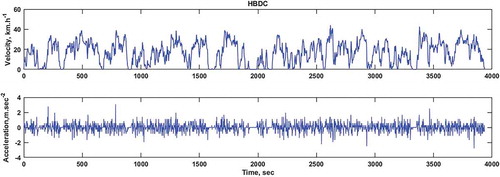
As shown on Figure 5, a bus in Hanoi has quite a large acceleration range, the change between acceleration and deceleration modes is continuous. This is in conformity with the characteristics of the traffic system in Hanoi with too many intersections, mixed traffic modes and the high vehicle density.

Evaluation of the driving cycle

To evaluate the obtained result, the developed HBDC cycle was compared with the real-world driving data. The comparison was based on the representative parameters (Table 6) and the VSP bins distribution (Figure 6), in which the definition of VSP bins follows that in the study of Hallmark and Qiu (2012).

Figure 6. Comparison of VSP bins distribution between the HBDC cycle and the real-world driving data.

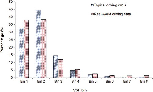
As shown in Table 6, the real-world driving characteristics of HBDC are closely matched with the real-world driving data, the acceleration range is quite large, and the time proportion of cruising mode is small. The relative deviation percentage between the HBDC cycle and the real-world driving data is quite small. The highest deviation is 27.44% for the cruising time parameter. In addition, as presented in Figure 6, the VSP bins distribution of the HBDC cycle is similar to the real-world driving data. The relative deviation percentage at the most concentrated bins being Bin 1, Bin 2, and Bin 3 are 7.2%, 7.3%, and 9.3%, respectively. The distribution of the VSP bins is uneven for both HBDC cycle and the real-world driving data. There are almost no VSP bins in the high VSP range. The proportion of negative VSP bins (Bin 1) is quite high, accounting for 32.7% and 37.8% in the HBDC and the real-world driving data, respectively.

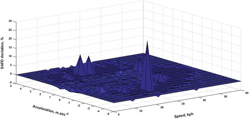
The SAFD also was used to evaluate the conformity of HBDC to the real-world driving data. The SAFD of HBDC is very similar to the SAFD of real-world driving data with fewer high-speed points but high almost zero-speed points (Figure 7). The difference in SAFD between HBDC and actual driving data is small because the picks on Figure 8 are very little and short. In the study of Ashtari, Bibeau, and Shahidinejad (2014), the SAFD_diff value was 14.2%, which is considered to be the smallest value in comparison with other studies. Therefore, the SAFD_diff obtained in this study, reaching to 13.2%, is reasonable. In other words, the HBDC can represent the real-world driving data.

Figure 7. Comparison of SAFD of the HBDC with the real-world driving data.

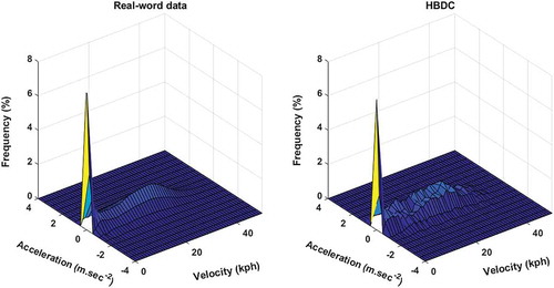
Figure 8. SAFD deviations between the HBDC and the real-world driving data.

Comparison with worldwide driving cycles

The comparison of the HBDC with other bus driving cycles is also presented in Figures 9 and 10. In Figure 9, the transit bus in Beijing is the city-specific driving cycle developed for the type of regular bus route with medium speed that is found in Beijing, China (Lai et al., 2013); the Braunschweig City Driving Cycle was developed at the Technical University of Braunschweig for an urban bus; the Transit Coach Operating Duty Cycle was originally designed for buses to measure fuel economy in United States; the New York Bus (NYBus) cycle was developed for heavy-duty vehicles, representative of the actual driving patterns of transit buses in New York City; the Manhattan cycle was developed for urban transit buses in the Manhattan core of New York City; the CBCD cycle is used to evaluate transit buses in the United States and Canada (Barlow et al., 2009; DieselNet, 2018).

Figure 9. Comparison of average speeds among different bus driving cycles.

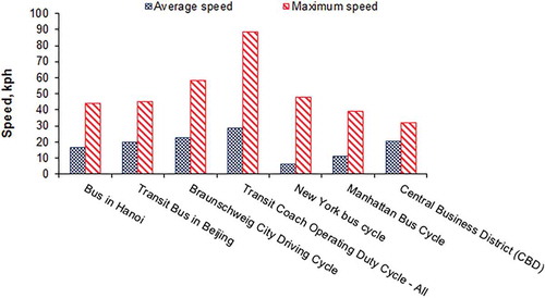
Figure 10. Comparison of time spent in different vehicle operating modes among different bus driving cycles.

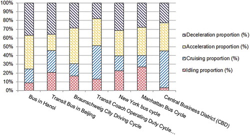
The average speed of the New York bus cycle is the smallest among the compared driving cycles as presented on Figure 9. The average speed of HBDC being 16.76 kph is quite high in comparison with other cycles. The maximum speeds of compared cycles fall in a large range, from 32 to 88 kph. The time proportions of different driving modes differ remarkably as stated in Figure 10. The idling time proportion of HBDC is only higher than that in the CBD cycle, but smaller than those in other cycles. The acceleration and deceleration time proportions of the HBDC are the highest due to traffic features in Hanoi as mentioned previously. In comparison with the driving cycle of intra-city buses in Chennai, India (Nesamani and Subramanian, 2011), the bus traffic in Hanoi seems to be more propitious because the idling time proportion of HBDC is 4.3 times smaller whereas the cruising time proportion is 3.4 times higher than those of the Chennai intra-city buses driving cycle.

Conclusion

The real-world driving characteristics of buses in Hanoi based on 317 trip segments, which were collected from the actual activities of buses on 15 bus routes, have been analyzed to determine representative variables for the driving cycle. A total of 14 representative driving parameters were selected from 33 driving cycle parameters using the HAC method. This study confirmed that the selected variables could be very different, even when applying the same data mining method on different data sets. Hence, future research investigations are recommended to determine the driving cycle representative variables based on their own input data instead of using results extracted from other studies. The typical driving cycle for the buses in Hanoi (HBDC was constructed using the Markov chain theory. The HBDC has a time duration of 3936 sec and an average velocity of 16.76 kph. The HBDC closely represents the overall real-world driving data with a percentage difference in SAFD of 13.2%, which is quite small in comparison with that of other studies. The developed HBDC, therefore, can be applied for the development of CSEFs for buses, which is a very good basis for integrated air quality management in Hanoi.

Acknowledgment

The authors would like to thank Mr. Emil Torp from Department of Electrical Engineering, Linköpings University, Sweden for his support in code developing of the driving cycle construction process.

Supplementary material

Supplemental data for this paper can be accessed on the publisher's website.

Additional information

Notes on contributors

Yen-Lien T. Nguyen

Yen-Lien T. Nguyen is a lecturer at the Faculty of Transport Safety and Environment, University of Transport and Communications, 3 Cau Giay, Hanoi, Vietnam.

Trung-Dung Nghiem

Trung-Dung Nghiem is an associate professor and dean of the School of Environmental Science and Technology, Hanoi University of Science and Technology, 1 Dai Co Viet, Hanoi, Vietnam.

Anh-Tuan Le

Anh-Tuan Le is a professor and dean of the School of Transportation Engineering, Hanoi University of Science and Technology, 1 Dai Co Viet, Hanoi, Vietnam.

Ngoc-Dung Bui

Ngoc-Dung Bui is a lecturer at the Faculty of Information Technology, University of Transport and Communications, 3 Cau Giay, Hanoi, Vietnam.

References

- Amirjamshidi, G., and M. J. Roorda. 2015. Development of simulated driving cycles for light, medium, and heavy duty trucks: Case of the Toronto Waterfront Area. Transp. Res. D 34:255–266. doi:10.1016/j.trd.2014.11.010.
- Ashtari, A., E. Bibeau, and S. Shahidinejad. 2014. Using large driving record samples and a stochastic approach for real-world driving cycle construction: Winnipeg driving cycle. Transp. Sci. 48 (2):170–183. doi:10.1287/trsc.1120.0447.
- Barlow, T. J., S. Latham, I. S. McCrae, and P. G. Boulter. 2009. A reference book of driving cycles for use in the measurement of road vehicle emissions. Published Project Report (PPR) 354, TRL limited.
- Bishop, J. D. K., C. J. Axon, and M. D. McCulloch. 2012. A robust, data-driven methodology for real driving cycle development. Transp. Res. D 17 (5):389–397. doi:10.1016/j.trd.2012.03.003.
- Brady, J., and M. O’Mahony. 2013. The development of a driving cycle for the greater Dublin area using a large database of driving data with a stochastic and statistical methodology. Proceedings of the ITRN2013, Trinity College Dublin.
- Bus-WebGPS. 2018. Bus operator management. Accessed May 25, 2018. http://dieuhanhxebuyt2.transerco.vn.
- Dai, Z., D. Niemeier, and D. Eisinger. 2008. Driving cycles: A new cycle-building method that better represents real-world emissions. Davis: Department of Civil & Environmental Engineering, University of California.
- DieselNet. 2018. Emission test cycles. Accessed May 10, 2018. https://www.dieselnet.com/standards/cycles/bac.php.
- Duarte, G. O., G. A. Gonçalves, and T. L. Farias. 2016. Analysis of fuel consumption and pollutant emissions of regulated and alternative driving cycles based on real-world measurements. Transp. Res. D 44:43–54. doi:10.1016/j.trd.2016.02.009.
- Duran, A., and M. Earleywine. 2012. GPS data filtration method for drive cycle analysis applications. Golden, CO: National Renewable Energy Lab (NREL).
- Ericsson, E. 2001. Independent driving pattern factors and their influence on fuel-use and exhaust emission factors. Transp. Res. D 6 (5):325–345. doi:10.1016/s1361-9209(01)00003-7.
- Franco, V., M. Kousoulidou, M. Muntean, L. Ntziachristos, S. Hausberger, and P. Dilara. 2013. Road vehicle emission factors development: A review. Atmos. Environ. 70:84–97. doi:10.1016/j.atmosenv.2013.01.006.
- GeoJson. 2018. Accessed May 10, 2018. http://geojson.io.
- Gubner, J. A. 2006. Probability and random processes for electrical and computer engineers. New York, NY: Cambridge University Press.
- Gujarati, D. N. 2004. Basic econometrics. 4th ed. New York, NY: McGraw-Hill.
- Guohua, S., Y. Lei, and T. Zhao. 2012. Distribution characteristics of vehicle-specific power on urban restricted-access roadways. J. Transp. Eng. 138 (2):202–209. doi:10.1061/(ASCE)TE.1943-5436.0000318.
- Haibo, Z., H. C Frey, and M. R Nagui. 2008. A vehicle specific power approach to speed- and facility- specific emissions estimates for diesel transit buses. Environ. Sci. Technol. 42 (21):7985–7991. doi:10.1021/es800208d.
- Hallmark, S., and Y. Qiu. 2012. Comparison of on-road emissions for B-0, B-10, and B-20 in transit buses. J. Air Waste Manage. Assoc. 62 (4):443–450. doi:10.1080/10962247.2012.658490.
- Hung, W. T., H. Y. Tong, C. P. Lee, K. Ha, and L. Y. Pao. 2007. Development of a practical driving cycle construction methodology: A case study in Hong Kong. Transp. Res. D 12 (2):115–128. doi:10.1016/j.trd.2007.01.002.
- Jimenez, J. L., P. McClintock, G. J. McRae, D. D. Nelson, and M. S. Zahniser. 1999. Vehicle specific power: A useful parameter for remote sensing and emission studies. Ninth CRC On-Road Vehicle Emissions Workshop, San Diego, CA.
- Jimenez-Palacios, J. L. 1999. Understanding and quantifying motor vehicle emissions with vehicle specific power and TILDAS remote sensing. Ph.D thesis, Massachusetts Institute of Technology, Cambridge, MA.
- Jun, J., R. Guensler, and J. Ogle. 2006. Smoothing methods designed to minimize the impact of GPS random error on travel distance, speed, and acceleration profile estimates. Transp. Res. Rec. 1972:141–150. doi:10.3141/1972-19.
- Lai, J., L. Yu, G. Song, P. Guo, and X. Chen. 2013. Development of city-specific driving cycles for transit buses based on VSP distributions: Case of Beijing. J. Transp. Eng. 139 (7):749–757. doi:10.1061/(ASCE)TE.1943-5436.0000547.
- Lavagnini, I., P. Pastore, and F. Magno. 1990. Comparison of the Kalman filter and dedicated algorithms for processing data for solution equilibria, noise smoothing and calibration. Anal. Chim. Acta 239. doi:10.1016/S0003-2670(00)83839-8.
- Le, A. T., M. T. Pham, T. T. Nguyen, and D. V. Nguyen. 2012. Measurements of emission factors and fuel consumption for motocycles on a chassis dynamometer based on a localized driving cycle. ASEAN Eng. J. C 1 (1):73–85.
- LEAD (Low Emissions Asian Development Program). 2013. Current challenges and priorities for greenhouse gas emission factor improvement in select Asian countries. United States Agency.
- Lee, T.-K., and Z. S. Filipi. 2011. Synthesis of real-world driving cycles using stochastic process and statistical methodology. Int. J. Veh. Des. 57 (1):17–36. doi:10.1504/IJVD.2011.043590.
- Lin, J. 2002. A Markov process approach to driving cycle development. Ph.D thesis, University of California, Davis.
- Lin, J., and D. A. Niemeier. 2002. An exploratory analysis comparing a stochastic driving cycle to California’s regulatory cycle. Atmos. Environ. 36 (38):5759–5770. doi:10.1016/S1352-2310(02)00695-7.
- Lin, J., and D. A. Niemeier. 2003. Estimating regional air quality vehicle emission inventories: Constructing robust driving cycles. Transp. Sci. 37 (3):330–346. doi:10.1287/trsc.37.3.330.16045.
- Lipar, P., I. Strnad, M. Česnik, and T. Maher. 2016. Development of urban driving cycle with GPS data ost processing. Promet Traffic Transp. 28 (4):353–364. doi:10.7307/ptt.v28i4.1916.
- Ministry of Transport. 2018. Hanoi: Renovation of public transport services. Accessed May 26, 2018. http://www.mt.gov.vn/vn/tin-tuc/53571/ha-noi–%C3%B0oi-moi-loai-hinh-dich-vu-van-tai-cong-cong.aspx.
- MONRE (Ministry of natural resources and environment). 2016. Vietnam state of environment 2016 - Urban environment. Vietnam.
- Nesamani, K. S., and K. P. Subramanian. 2011. Development of a driving cycle for intra-city buses in Chennai, India. Atmos. Environ. 45 (31):5469–5476. doi:10.1016/j.atmosenv.2011.06.067.
- Nguyen, T. Y. L., and T.-D. Nghiem. 2017. The determination of driving characteristics of Hanoi bus system and their impacts on the emission. J. Sci. Technol. 55 (1):74–83. doi:10.15625/0866-708X/55/1/8398.
- Niemeier, D. A., T. Limanond, and M. E. Jennifer. 1999. Data collection for driving cycle development: Evaluation of data collection protocols. Department of Civil and Environmental Engineering, Institute of Transportation Studies, University of California at Davis.
- Perhinschi, M. G., C. Marlowe, S. Tamayo, T. Jun, and W. W. Scott. 2011. Evolutionary algorithm for vehicle driving cycle generation. J. Air Waste Manage. Assoc. 61 (9):923–931. doi:10.1080/10473289.2011.596742.
- Qi, Y., A. Padiath, Q. Zhao, and L. Yu. 2016. Development of operating mode distributions for different types of roadways under different congestion levels for vehicle emission assessment using MOVES. J. Air Waste Manage. Assoc. 66 (10):1003–1011. doi:10.1080/10962247.2016.1194338.
- Saleh, W., R. Kumar, H. Kirby, and P. Kumar. 2009. Real world driving cycle for motocycles in Edinburgh. Transp. Res. D 14 (5):326–333. doi:10.1016/j.trd.2009.03.003.
- Selesnick, I. 2013. Estimate missing data by least squares: Minimize the energy of second-order derivative subject to the data consistency constraint. Accessed April 21, 2017. http://eeweb.poly.edu/iselesni/lecture_notes/least_squares/LeastSquares_SPdemos/missing_data/html/missing_data_demo.html.
- Shi, Q., Y. Zheng, R. Wang, and Y. Li. 2011. The study of a new method of driving cycles construction. Procedia Eng. 16:79–87. doi:10.1016/j.proeng.2011.08.1055.
- Shi, S., N. Lin, Y. Zhang, J. Cheng, C. Huang, L. Liu, and B. Lu. 2016. Research on Markov property analysis of driving cycles and its application. Transp. Res, D 47:171–181. doi:10.1016/j.trd.2016.05.013.
- Tong, H. Y., H. D. Tung, W. T. Hung, and H. V. Nguyen. 2011. Development of driving cycles for motorcycles and light-duty vehicles in Vietnam. Atmos. Environ. 45 (29):5191–5199. doi:10.1016/j.atmosenv.2011.06.023.
- Tong, H. Y., and W. T. Hung. 2010. A framework for developing driving cycles with on-road driving data. Transp. Rev. 30 (5):589–615. doi:10.1080/01441640903286134.
- Torp, E., and P. Önnegren. 2013. Driving cycle generation using statistical analysis and Markov chain. Sweden: Department of Electrical Engineering, Likopings University.
- Transerco Transportation Service Corporation. 2018. Accessed May 10, 2018. http://transerco.com.vn.
- US. EPA (United State Environmental Protection Agency). 2010. MOVES and related models. Accessed November 20, 2017. https://www.epa.gov/moves/moves2014a-latest-version-motor-vehicle-emission-simulator-moves#manuals.
- Watson, H. C., E. E. Milkins, and V. Bulach. 1976. How sophisticated should a vehicle emissions model be. Clean air society of Australia and New Zealand Smog’76 conference workshop paper, Sydney, Australia.