Trends in passenger exposure to carbon monoxide inside a vehicle on an arterial highway of the San Francisco Peninsula over 30 years: A longitudinal study

ABSTRACT

This paper describes a long-term trend study of passenger exposure to carbon monoxide (CO) inside a vehicle traveling on an arterial highway in northern California. CO exposure was measured during four field surveys on State Route #82 (El Camino Real) on the San Francisco Peninsula in 1980–1981, 1991–1992, 2001–2002, and 2010–2011. Each field survey took at least 12 months. Fifty trips from each survey—for a total of 200 trips—were matched by date, day of the week, and starting time of the day to facilitate comparisons over three decades. The mean net CO concentration of each trip was obtained by subtracting the background CO level from the average CO concentration for the entire trip. The mean net CO concentration (0.5 ppm) for 2010–2011 was only 5.2% of that (9.7 ppm) for 1980–1981. For the 50 trips, the average travel time for the 1980–1981 period (39.6 min) was only 8.3% higher than during the 2010–2011 period (36.3 min). The estimated round-trip distance on the highway was held constant at 11.8 miles. The reduction in the mean net CO concentration was attributed to more stringent CO emission standards on new vehicles sold in California since 1980. The state’s cold-temperature CO standard implemented in 1996 appeared to reduce high CO concentrations that were observed during the late fall and winter of 1980–1981. In addition, the observed standard deviation in concentration fell from 3.1 ppm in 1980–1981 to 0.2 ppm in 2010–2011, and the range of the 50 mean net CO concentrations narrowed from 14.9 ppm in 1980–1981 to 1.1 ppm in 2010–2011, but the relative variability, as indicated by the geometric standard deviation, remained the same. These results have important scientific implications for regulatory policies designed to control air pollution from motor vehicles.

Implications: Many developing countries launched or expanded their mobile source emission control programs in the 1990s, yet many of them do not have adequate inspection and maintenance (I/M) programs. The El Camino Real study shows the long-term public health benefits of more stringent motor vehicle emission standards for carbon monoxide (CO) on new cars and of an I/M program (Smog Check) on the existing fleet in California. The study provides a protocol for conducting standardized field surveys of in-vehicle exposure on a periodic basis. Such surveys would enable developing countries to assess the progress of their mobile source emission control programs.

Introduction

Motor vehicles emit carbon monoxide (CO) from their tailpipes as a by-product of incomplete fuel combustion, particularly fuels that contain elemental carbon, such as gasoline and diesel. The Clean Air Act (CAA) amendments of 1970 and 1990 stipulated progressively tighter standards on tailpipe emissions from passenger cars. These standards were achieved through various emission control programs and clean-fuel technologies (Walsh 1999). To achieve these standards, automobile manufacturers developed catalytic converters, which became standard equipment on new passenger cars sold in the United States during the 1975 model year. As the proportion of vehicles on the road with catalysts increased, regulators assumed that air quality in metropolitan areas would improve through the process of “fleet turnover.” For air pollutants such as CO, total emissions from on-road vehicles and ambient concentrations of mobile-source air pollutants have declined in the United States. The number of fixed-site monitoring stations showing violations of the National Ambient Air Quality Standards (NAAQS) for CO has fallen substantially from the early 1970s, when CO monitoring became widespread. The U.S. EPA has posted a website (https://www.epa.gov/air-trends/carbon-monoxide-trends) that shows a downward trend in nationwide ambient CO concentrations since 1970. This success was achieved even as the U.S. population grew 58% between 1970 and 2016 and the country’s total vehicle miles of travel (VMT) grew 190% during that 46-yr period (U.S. Environmental Protection Agency 2017).

Yet studies have shown that CO concentrations measured at ambient air quality monitoring stations do not adequately represent CO exposures in microenvironments associated with motor vehicles, such as parking garages and traffic intersections (Flachsbart 1999). A microenvironment is “a chunk of air space with homogeneous pollutant concentration” (Duan 1982, 305). Large-scale field studies of population exposure to CO in Denver, CO, and Washington, DC, revealed that traveling long distances by automobile is likely to elevate one’s personal exposure to CO concentrations, and that these concentrations were substantially higher than ambient CO concentrations measured concurrently at fixed-site monitors (Akland et al. 1985). Unlike fixed-site monitoring of ambient air quality, the CAA does not require periodic field studies of population exposure to CO, even though exposure scientists consider personal exposure to be a better indicator than ambient measurements of the health risks related to CO emissions (Flachsbart 2007). Sections 108 and 109 of the CAA require an assessment of the latest, relevant scientific information that may affect the U.S. EPA’s periodic review of the NAAQS for a criteria air pollutant. This assessment typically includes a review of human exposure to the air pollutant, which is evident in the two most recent reports for CO (U.S. Environmental Protection Agency 2000, 2010). The 2000 Air Quality Criteria for CO document actually has more discussion of exposure studies that are relevant to our 30-yr longitudinal study than does the 2010 Integrated Science Assessment (ISA) for CO. The 2010 ISA report makes this statement: “Previous studies in the 1980s and 1990s, when ambient levels were higher, involved successful deployment of these [personal] monitors, but more recent exposure studies have avoided personal CO measurements because there are now a high percentage of nondetects” (U.S. Environmental Protection Agency 2010, 3–91).

A study by Rodes et al. (1998) represents an example of an exposure study using personal monitors in the late 1990s. They conducted in-vehicle field surveys in two California cities during early fall of 1997. The surveys purposely focused on driving scenarios likely to result in exposure to high concentrations of several air pollutants including CO inside a test vehicle. Continuous CO concentrations were measured over 2-hr periods at different times of day for 29 trips by two test vehicles (one vehicle following the other). They reported that average net CO concentrations were higher in Los Angeles (4.6–4.9 ppm) than in Sacramento (2.1–3.1 ppm) during a limited number of rush-hour trips on freeways. They found little difference in average CO concentrations between freeway and arterial trips during rush-hour drives in both cities. Based on preliminary analysis of five trips, the study reported that CO concentrations could reach short-term peaks, ranging from approximately 15 to 70 ppm, when the lead test vehicle trailed gasoline-powered delivery trucks and older sedans. We expect some results of the Rodes et al. (1998) study to differ from our field surveys on El Camino Real, because the two studies used different methods of data collection.

The lack of recent in-vehicle CO measurements during the last 10 yr is apparent from recent reviews of the literature on personal exposure to air pollution (de Nazelle, Bode, and Orjuela 2017; Xu, Xiaokai, and Xiong 2018). The focus of recent studies appears to be on human exposure to particulate matter and other air pollutants. An article by de Nazelle, Bode, and Orjuela (2017) reviewed the published literature on measurements of exposure to air pollutants on various transportation modes in European cities and reported a CO mean exposure of 7 ppm in cars in Barcelona, Spain, in 2009, with lower CO concentrations observed in a car in London, UK (1.3 ppm), in 2003. Xu, Xiaokai, and Xiong (2018) reviewed more than 90 studies of air pollutant concentrations measured inside motor vehicle cabins in 10 countries, but their review focused on pollutants other than CO. We could not find any other recent systematic studies of in-vehicle exposure to CO to compare with our study results, even though CO is one of six major air pollutants controlled in the United States.

Although there is no legal mandate to measure personal exposure, there are indications that CO exposure measured inside motor vehicles traveling on highways in the United States has improved. A seminal review of 16 in-vehicle exposure studies performed in various U.S. cities between 1965 and 1992 found that passenger-cabin exposures to CO fell 92% during that 27-yr period (Flachsbart 1995). This trend was consistent with improvement in ambient CO concentrations in urban areas as noted in the preceding. However, only two of those 16 studies used a standard protocol. For most of those studies, typical in-vehicle CO exposures varied by study approach, the urban location of the study, season of the year, roadway type and location, travel mode, and the ventilation settings of the test vehicle. The review recommended that future studies use standard methods to “improve their potential to assess the effectiveness of public policies in curtailing automotive emissions over the long term.” (Flachsbart 1995, 493) This recommendation was endorsed by two later publications (U.S. Environmental Protection Agency 2000, 4–31; Flachsbart 2007, 136). A more recent review advocated that in-vehicle CO exposure studies precisely describe testing conditions and use strict quality assurance and control procedures to make it easier “to generalize findings and compare between studies” (El-Fadel and Abi-Esber 2009, 615).

Consequently, we conducted a longitudinal study of passenger exposure to CO inside a vehicle on an arterial highway (El Camino Real) of the San Francisco Peninsula in Northern California. (This paper uses the terms “passenger exposure” and “in-vehicle concentration” to mean the same thing.) El Camino Real connects several cities in the counties of San Mateo and Santa Clara on the San Francisco Peninsula. The results of this longitudinal study, as reported in this paper, offer evidence of the effectiveness of California’s motor vehicle emission control program between 1980 and 2010. The paper also illustrates the use of a statistical model to predict the distribution of roadway exposures measured during field surveys based on reasonable estimates of tailpipe emissions on the roadway. Our hypotheses are (1) that the arithmetic mean of the in-vehicle CO exposures measured during each field survey is proportional to the estimated annual average of the CO exhaust emission rate on the roadway, and (2) that the geometric standard deviation of the frequency distribution of CO exposures is the same for each field survey. The study discussed in this paper is an extension of two earlier studies of the same site over an entire decade (Ott 1993; Yu, Hildemann, and Ott 1996). This paper is the only known long-term trend study of passenger CO exposure in the United States using a set of matched data over three decades.

The San Francisco Peninsula

The combined population of the counties of San Mateo and Santa Clara on the San Francisco Peninsula increased from 1.88 million in 1980 to 2.50 million in 2010, an increase of about 33% in 30 yr (Cox, Delao, and Komorniczak 2013; Cox et al. 2007). In spite of this increase in population, trends in ambient CO indicators showed substantial improvement in these two counties over this 30-yr period (Table 1) (Alexis et al. 2001; Cox, Delao, and Komorniczak 2013). This improvement resulted from an 88.3% decline in CO emissions from gasoline vehicles in the San Francisco Bay Area Air Basin. In this region, gasoline vehicles accounted for 91.2% of CO emissions from all sources in 1980, but were projected to be 54.9% of all sources in 2010 by the California Air Resources Board (Table 2). This emission reduction has been attributed, in part, to more stringent motor vehicle exhaust emission standards phased in on new cars and trucks sold in California since 1966 (California Air Resources Board 1997), and to state implementation in 1984 of an inspection and maintenance program known locally as Smog Check (Eisinger 2010). Beginning with the 1996 model year, California implemented a cold-temperature CO emission standard for new cars. The cold-temperature standard allowed 10 g/mile measured at 20°F, rather than at the 75°F temperature used for the Federal Test Procedure (FTP).

Table 1. Indicators of ambient CO air quality for two counties on the San Francisco Peninsula during the first year of each survey period.

	1980	1990	2000	2010
San Mateo County
Peak 8-hr indicator (ppm)	9.4	5.9	4.4	1.9
Maximum 1-hr concentration (ppm)	13.0	12.0	9.8	3.3
Maximum 8-hr concentration (ppm)	8.3	5.9	4.4	1.7
Days above state 8-hr standard	0	0	0	0
Days above national 8-hr standard	0	0	0	0
Santa Clara County
Peak 8-hr indicator (ppm)	15.5	12.6	7.1	2.5
Maximum 1-hr concentration (ppm)	27.0	18.0	8.9	2.5
Maximum 8-hr concentration (ppm)	16.4	11.0	7.0	2.2
Days above state 8-hr standard	16	4	0	0
Days above national 8-hr standard	12	2	0	0

Note. Sources: Alexis et al. (2001); Cox, Delao, and Komorniczak (2013).

Table 2. CO emissions (tons per day, annual average) for the San Francisco Bay Area by decade.

	1980	1990	2000	2010
Stationary sources	55	65	50	38
Area-wide sources	135	160	169	182
On-road mobile	7615	4446	2203	914
Gasoline vehicles	7597	4414	2177	889
Diesel vehicles	18	32	26	25
Other mobile	529	654	539	484
All sources	8334	5325	2961	1618

Note. Source: Cox et al. (2007, 4–26).

Study design

The design of the study adhered to the “max-min-con” principle of research design. This principle has three goals (Kerlinger 1986; Tashakkori and Teddlie 1998). The first goal is to maximize variation in the independent variable (i.e., time), recognizing that time is a surrogate for the effects of emission standards and control programs. We assumed that the cumulative effects of these standards and programs on passenger CO exposure (i.e., the dependent variable) would be apparent and easier to detect after a long period of time. Hence, the study used a longitudinal design spanning three decades to determine the effect of California’s motor vehicle emission control program on in-vehicle CO exposure. The second goal is to minimize error by carefully calibrating monitors using reference gases and recording background CO concentrations at a location off the arterial highway where passenger exposure was measured. The third goal is to control variables that could also explain passenger exposure, such as (a) average trip duration and speed, (b) the percentage of time spent at traffic lights, (c) the ventilation of the test vehicle, (d) trip date and starting time, and (e) travel mode. In effect, the purpose of the third goal is to at least measure, if not control, variables that might also affect the dependent variable to rule out competing explanations of the results.

Using personal monitors, CO exposure was measured and logged at least once every 12 sec inside a motor vehicle during trips on the study site (El Camino Real). Each field survey occurred during a 13- to 15-month period, from early January through either February or March of the following year, for four different time periods: 1980–1981, 1991–1992, 2001–2002, and 2010–2011. A standard protocol was used during each survey period to control for the effects of potential confounding variables that were shown by a previous study to be strongly associated with CO exposure inside an automobile traveling on an urban arterial highway (Ott, Switzer, and Willits 1994). The sections that follow provide further details about the study site, data collection methods, quality assurance procedures, and trip screening criteria of the field surveys to support the purpose of this paper. A 93-page technical report provides more details about the initial field survey in 1980–1981 (Ott, Switzer, and Willits 1993).

Study site

The study site was a 5.9-mile segment of State Route #82 (El Camino Real), a major arterial highway near Stanford University on the San Francisco Peninsula. The site, which includes portions of both San Mateo and Santa Clara counties, is four lanes (two in each direction) in San Mateo County and six lanes (three in each direction) in Santa Clara County. From the starting point at Cambridge Ave. in Menlo Park at the southern end of San Mateo County, the driver proceeded southeast on the highway, entering Santa Clara County at the Palo Alto border. At San Antonio Rd., which defines a border between Palo Alto and Mountain View, the driver made a U-turn and drove northwest on the highway. Upon reaching Encinal Dr. in Menlo Park, the driver made another U-turn and drove southeast again. Except for U-turns, the driver usually stayed in the middle lane. Near the end of each trip at Harvard Ave., which is a quiet residential street in Menlo Park, the driver made a right turn and drove about 300 ft from the highway before parking the vehicle. The total trip distance on the study site, which did not include Harvard Ave., was estimated at 11.8 miles according to the vehicle’s odometer.

Based on data from R. L. Polk & Co., Yu, Hildemann, and Ott (1996) reported that the percentage of total registered passenger vehicles by model year from 1976 through 1989 for Santa Clara County resembled the composition of both the state of California and the entire United States. This indicated that the motor vehicle population of Santa Clara County could be representative of other locations and jurisdictions. (See “CO exhaust emission rates” section for further discussion of whether the study site is representative of other jurisdictions, based on their CO exhaust emission rates from 1990 through 2010.)

The number of intersections with traffic signals increased on the study site from 19 in 1980–1981, to 23 in 1991–1992, to 27 in 2001–2002, and to 28 in 2010–2011. The California Department of Transportation (Caltrans) routinely collects data to determine the average daily traffic (ADT) volumes on State Route #82. During the study period, the annual ADT was available both forward and back at six major intersections on El Camino Real for 1980, 1991, 2001 and 2010. These intersections, which include San Antonio Rd., Charleston Rd., Page Mill Rd., Embarcadero Rd., the University Ave. overpass, and Santa Cruz Ave., represent nearly the entire length of the study site. The annual ADT varied by intersection and by study period. Annual ADT ranged from a low of 32,500 vehicles as determined for two sites, one north of Embarcadero Rd. and another south of University Ave. in 1980, to a high of 54,000 vehicles for a site south of Charleston Rd. in 2001. Between 1980 and 2010, the annual ADT on the study site increased from 3.9% to 19.1% at eight locations south of the University Ave. intersection, decreased from 15.6% to 25.0% at three locations north of University Ave., and did not change just north of the Page Mill Rd. intersection (California Department of Transportation 2017; Kyutoku 2002).

Data collection methods

At least one trip was made nearly every week during the 13- to 15-month survey period. Although trips were taken on different days of the week and at different times of the day, selection of trip dates and trip-starting times was not a random process. Most trips occurred on Friday morning between 10:00 a.m. and 12:00 noon. Sometimes two trips were taken, one immediately after the other, to examine the difference in CO exposures on two drives under approximately the same weather conditions and expected differences in traffic conditions. In addition, various other weekdays and starting times were selected to observe their effect on potential passenger exposure. We are referring to the exposure as “potential” only because the measurements are made inside the car’s passenger compartment and not by using a monitor that was directly worn by the driver or passenger.

The driver (Wayne Ott) recorded the starting and ending times of each trip so that the total trip duration in minutes and seconds and the average speed of the trip could be determined. During each trip, the driver attempted to maintain the speed of surrounding traffic on the highway, which typically ranged from 30 to 40 mph when traffic was moving. The driver also recorded the amount of time spent stopped at traffic lights and counted the number of vehicles surrounding the test vehicle while stopped. At the end of the trip, the driver measured the background CO concentration in parts per million (ppm) outside the test vehicle about 5–10 min after parking the car on Harvard Ave., at least 300 ft from the study site on El Camino Real. The driver received assistance from a passenger, who rode in the right front seat for every trip during Survey #1 (1980–1981), because the CO exposure monitors during that survey period did not have an automatic data logger.

Each field survey took advantage of technical advances made in personal exposure monitors and data logging systems over the course of the study. During Survey #1 (1980–1981), CO concentrations were measured using a General Electric CO “detector” (model 15ECS3CO1). Several early trips during this period used a high-time resolution ECOlyzer 9000 “dosimeter” made by Energetics Science, Inc. Data from both instruments were recorded on an Esterline-Angus “Miniservo” strip-chart recorder. The strip-chart data were later digitized manually at 12-sec intervals. During Survey #2 (1991–1992), the Langan L15 and Draeger 190 electrochemical CO monitors—each with internal data loggers—were used. The stored data from the Langan monitor were transferred by cable to a Macintosh personal computer using Sense-Your-World software supplied by the manufacturer. The Draeger monitor required an interface adapter attached to an IBM personal computer. Measuring low CO concentrations during Survey #3 (2001–2002) and Survey #4 (2010–2011) required two Langan T15n Enhanced CO Measurers with internal DataBear loggers (Langan Products, San Francisco, CA). The sampling rates of the instruments were set for once every 2 sec during Survey #2, once every 12 sec during Survey #3, and once every 10 sec during Survey #4. The Langan monitor uses an internal HOBO data logger (Onset Corp., Bourne, MA). The data were downloaded after each trip into spreadsheet files on a Mac personal computer for further analysis.

At the beginning of Survey #2, an experiment was performed to compare instruments used during Survey #1 with those used during Surveys #2, #3, and #4. The test vehicle equipped with four monitors drove six loops of a route in downtown San Francisco on January 31, 1991. Each loop included the Broadway Tunnel, a “street canyon” on Montgomery St. in the Financial District, the Stockton Tunnel, and a roadway relatively free of traffic (i.e., Union St. from Stockton St. to Larkin St.). Ott reported that CO concentrations measured by the four monitors “seldom differed by more than 0.5 ppm and that the one-minute averages were highly correlated” (Ott, Switzer, and Willits 1993, 5). This experiment was not repeated at the start of Surveys #3 and #4, because the monitors used during the second, third, and fourth survey periods were similar instruments made by Langan Products, Inc.

During each field survey, the CO monitors sat on the right front passenger seat of the test vehicle. Each field survey used the same driver but different test vehicles. Specifically, a 1974 Volkswagen Model 412 served as the test vehicle during Survey #1, a 1986 Mazda Model 626 was used during Survey #2, a 1999 Lexus sport utility vehicle (SUV) was driven during Survey #3, and a 2008 Toyota Prius was used during Survey #4. Because of this variation, experiments were conducted on the vehicle to measure its air-exchange rate and to establish that its exhaust system did not leak into the passenger compartment. To detect exhaust leakage, at least one full trip during each survey period was taken at 2:00 a.m. when there was virtually no traffic on the highway. The CO monitor and its data logger were operated in the same manner regardless of whether the trip was taken at 2:00 a.m. or during daylight hours. Since there was virtually no traffic on the roadway at 2:00 a.m., the CO concentrations measured inside the vehicle were either zero or equal to the background level. These tests detected no leakage of CO concentrations from the vehicle’s own exhaust system. The data on passenger CO exposure for these four early-morning trips are not included in the results reported in the following.

On the other hand, Ott, Switzer, and Willits (1993) confirmed our expectations at the beginning of the study in 1980 that window positions on the vehicle would affect its air-exchange rate. A later and more extensive study showed the effects of speed, ventilation, and window position on the air-exchange rates of the four test vehicles (Ott, Klepeis, and Switzer 2008). Consequently, the position of each window was standardized on all trips on each survey as follows: left-front window completely open; right-front window open three inches; rear windows closed; and the mechanical ventilation system turned off. Ott, Switzer, and Willits (1994) showed that the interior and exterior average concentrations measured over the entire trip under these conditions were approximately the same. This occurs if the product of the instantaneous interior concentration at the end of the trip and the residence time (i.e., the time constant) is small relative to the total time of the trip. (The vehicle’s “residence time” is the reciprocal of the vehicle’s air-exchange rate.)

There were no changes in the in-vehicle filtration systems employed in our field studies. The ventilation fans in our test vehicles were always off. Fortunately, winters are fairly mild in California, but even in winter the heating system was always off. Even in cool weather or during rain, the window positions, which affect the air-exchange rate of the vehicle, were always the same (i.e., driver’s window completely open, passenger window open 3 inches, and rear windows closed). Fixing the heating, ventilation, and window position settings is important to enable long-term studies to compare their results over time.

Quality assurance procedures

Each CO monitoring instrument was carefully calibrated using a certified calibration gas for the “zero” value and a certified calibration gas for the “span” value. This calibration occurred within 30 min of the start of each trip or pair of trips made on a given day. These gases were traceable to the National Institute of Standards and Technology (NIST) certified gases. The Langan monitors used in the second, third, and fourth field surveys kept an internal digital record of ambient temperatures. If the Langan monitor is operated within a few degrees of 20°C (68°F) temperature, there is essentially no thermal impact on the monitor’s CO measurement (Langan 2006). The ambient temperatures at the calibration location and at the roadway study site were typically within ±4°C (±7.2°F) of each other, and the whole process of calibrating the instruments and collecting the in-vehicle CO concentrations took less than 90 min for most trips. Because the ambient temperatures during calibration and driving were essentially the same, the CO concentrations measured by these monitors did not need to be adjusted for daily change in ambient temperature. Also, no heating or air-conditioning systems were used inside the test vehicle during any of the trips.

In the 1980–1981 and 1991–1992 field surveys, commercially available span gases of “53 ppm” and “60 ppm” were used. The latter gas was preserved for comparison with the reference gases used in the third field survey in 2001–2002 and the fourth field survey in 2010–2011. In a special quality assurance evaluation, nine span reference gases ranging from 20 to 60 ppm were obtained from commercial sources (Air Liquide Calgaz, Scott Specialty Gas Co., Alphagaz, General Electric Co., Eco-Span, Bryne Specialty Gas Co., Express Gas), including a Calgaz NIST-traceable reference gas (Ott et al. 1995). Their values were verified and compared by gas chromatography using a reduction gas analyzer (Trace Analytical, Inc., Menlo Park, CA). These span reference gases were found to be consistent with their nominal values to within ±2 ppm or ±3.3%. The gas chromatography analysis allowed the reference gas concentrations of these gases to be redefined and improved to a greater precision of within ±0.1 ppm using the NIST gas as the primary reference gas. In the 2001–2002 field survey, a nominal 20 ppm Alphagaz reference gas was used (redefined as nominal value of 19.9 ppm) throughout the survey, and the zero gas was generated using a Hopcalite heater-generator system attached to a 100-cc/min constant-flow pump. These quality assurance steps were necessary partly because of the extremely low CO concentrations found on the highway during the 2001–2002 field survey, which were even lower during the 2010–2011 field survey.

Before each trip, the zero gas was attached to the intake of each monitor and allowed to flow for 2–3 min until a stable reading was obtained on the data logger, with the values recorded on the log sheet. Next, the span gas was attached with a cylinder regulator of 100 cc/min; a stable span reading was obtained on the monitor’s digital display after 2–3 min. If the span gas and the instrument reading on the digital display differed by more than 2 ppm, the calibration set-screw potentiometer on the monitor was adjusted to make the difference as close to zero as possible (generally less than 0.5 ppm), and the resulting values were recorded on the survey log sheet. With a 60-ppm calibration gas, 0.5 ppm is less than 1% error. The linearity of the electrochemical monitors and their sensitivity to interference were evaluated in the laboratory using a reduction gas chromatograph analyzer (Ott et al. 1995).

The 2010 CO Integrated Science Assessment provides general information on CO monitors, including the Langan CO monitor, but little information is given about their sensitivity to low concentrations. For example, the authors of the 2010 CO ISA do not mention that the Langan CO monitors have two different resolution settings that the user can select by changing a jumper on the internal circuit board (Langan 2006). The high-resolution setting multiplies the readings by 10.0, causing more numerals to appear to the right of the decimal place. All of the trips on the El Camino study site in the 2010–2011 field survey used two Langan CO monitors, one as the main monitor and the other as a backup monitor. Because of the low CO concentrations observed on the highway during that survey period, the jumper wires of both monitors were set to their high-resolution settings. This adjustment enabled us to record readings to four decimal places, which could be rounded to tenths of a part per million.

Trip screening criteria

The number of trips taken during each survey period varied: 93 trips were taken during Survey #1, 131 trips during Survey #2, 60 trips during Survey #3, and 50 trips during Survey #4. Of the 93 trips taken during Survey #1, 88 trips employed a standard window position as described earlier. Using data from the 88 trips of Survey #1, Ott, Switzer, and Willits (1994) used multivariate regression models to evaluate the explanatory power of nine potential covariates of in-vehicle CO exposure.These variables included ambient CO concentrations at two nearby fixed-site monitors, atmospheric stability, a seasonal trend function, time of day of the drive, average surrounding vehicle count, trip duration, proportion of time stopped at traffic lights, and instrument type. The variables most highly correlated with the average CO concentration of each trip were three variables (surrounding vehicle count, proportion of time stopped at traffic lights, and trip duration). In fact, all three variables were highly correlated with each other, because all of them were probably affected by traffic conditions on the highway. The variables least correlated with exposure were atmospheric stability and the time of day of the drive (Ott, Switzer, and Willits 1993, 1994).

For the 1980–1981 data, a powerful yet parsimonious model (adjusted R² = 0.672) predicted the average in-vehicle CO exposure per trip as a function of just two variables (Ott, Switzer, and Willits 1994). These were traffic conditions, as measured by the proportion of travel time stopped, and a seasonal term expressed as a cosine function of the day of the year on which the trip was taken. The trip average CO concentration tended to be higher from late fall through early spring (November through March) of that time period and lower during the late spring and summer months (May through August). It was clear that the seasonal term had captured variation in weather variables (e.g., ambient temperature, wind speed, atmospheric stability, etc.). However, it was also possible that the seasonal term represented seasonal variation in traffic conditions. A model that included ambient CO concentrations from a fixed-site monitor slightly improved the power of the model (adjusted R² = 0.708).

As stated in the preceding, one purpose of the present study was to determine the long-term effect of California’s motor vehicle emission control program on passenger CO exposure. To achieve this goal, the study design attempted to minimize the confounding effects of weather and traffic variables on exposure. To minimize the effects of these variables, trips were matched by travel date and starting time to form a “case.” Each case consisted of four trips—one selected from each survey period (i.e., 1980–1981, 1991–1992, 2001–2002, and 2010–2011). Each case satisfied the following three criteria:

1. Matched trips occur on the exact same day of the week (e.g., all four trips of a case occur on a Friday), given that traffic and weather conditions vary by day of the week.

2. Matched trips occur within 14 days of the survey date’s serial day of a Julian calendar year, given that traffic volumes (e.g., ADT) and weather conditions (e.g., temperature) vary seasonally.

3. The starting time of matched trips occur within 95 min of each other, given that traffic congestion and weather conditions (e.g., temperature) vary by hour of the day.

By the end of the fourth field survey, 50 cases of matched trips satisfied these three criteria.

Results and discussion

This section reports and discusses results for net in-vehicle CO exposure, indicators of traffic conditions on the study site, and the statistical rollback model. A tabulation of the dates and starting times of all 50 cases revealed that 80% of them (40 cases) occurred on Fridays. Morning trips (i.e., trips starting between 7:45 a.m. and 12:00 noon) represented between 62% and 70% (between 31 and 35 cases) of the 50 cases, depending on the survey period. The starting times of afternoon trips, which occurred between 12:00 noon and 6:20 p.m., accounted for all other trips.

Net in-vehicle CO exposure

The background CO concentration in the ambient air was measured at the end of each trip about 300 ft off the El Camino Real study site. Even though the background CO concentration was small (usually less than 1.0 ppm), it was subtracted from the average CO concentration inside the vehicle for the entire trip to determine the net CO trip average concentration. The purpose of this calculation was to factor out the effect of ambient CO concentrations (Flachsbart 2007, 128). Table 3 shows descriptive statistics for measured net in-vehicle CO concentrations based on 50 matched cases from each field survey.

Table 3. Descriptive statistics of measured net in-vehicle CO concentrations (ppm) for four field surveys based on 50 matched cases from each survey.

Field survey	Mean net CO concentration (ppm)	Standard deviation (ppm)	Median net CO concentration (ppm)	Range of the 50 mean net CO concentrations (ppm)
#1: 1980–1981	9.7	3.1	9.2	4.2–19.1
#2: 1991–1992	4.8	1.7	4.8	1.2–11.0
#3: 2001–2002	1.7	0.8	1.5	0.4–5.3
#4: 2010–2011	0.5	0.2	0.5	0.2–1.3

The mean net CO exposure of the 50 trips taken during the 2010–2011 period was 0.5 ppm, which was about 29% of the corresponding mean of 1.7 ppm for the 2001–2002 period. In turn, the 2001–2002 mean of 1.7 ppm was about 35% of the mean for the 1991–1992 period (4.8 ppm) and about 18% of the mean for the 1980–1981 period (9.7 ppm). Overall, the observed mean of the net CO concentrations decreased 95% over three decades, from 9.7 ppm for the 1980–1981 period to 0.5 ppm for the 2010–2011 period. All in-vehicle CO concentrations reported in this paper are net CO exposures.

Our study represents an example of an ex post facto research design, which assumes that two or more samples are randomly drawn from different populations. Ordinarily, a one-way analysis of variance (ANOVA) is appropriate for testing the hypothesis that the four field surveys were drawn from populations having the same mean net CO concentration. However, our CO concentration data do not satisfy two assumptions of the ANOVA F-test: (1) homoscedasticity of the dependent variable (equality of variances among the four groups), and (2) that the dependent variable is normally distributed within each group. Consequently, we did a Kruskal–Wallis H-test, which is a nonparametric alternative to the ANOVA F-test. The H-test does not require normality of distribution or homogeneity of variance in our data. The Kruskal–Wallis H-test is almost as powerful as the ANOVA F-test. The H-test determines whether the total ranks in two or more independent groups are significantly different. The H-test statistic must be corrected for tied ranks and can be compared to critical values of a chi-squared distribution (Roscoe 1975, 304–308; Privitera 2012, 600–603). For our data, the value of H (corrected for tied ranks) was equal to 176.232, which exceeds the critical chi-squared value of 16.266 for a p value of 0.001 for three degrees of freedom. The corrected value of H represented only a slight adjustment for tied ranks for our data. Therefore, there appears to be a significant difference in the ranks of the data from our four field surveys, with a very low probability (0.001) of rejecting a true null hypothesis.

The reduction in mean net CO concentrations during these three decades may be attributed to the phasing in of more stringent motor vehicle exhaust emission standards for new cars and trucks sold in California over this period. Table 4 shows these standards for the state of California and the other 49 states. The table shows that California lowered the CO exhaust emission standard from 9 g/mile in 1980 to 1.7 g/mile for the 2003 model year. Moreover, the higher CO concentrations observed during late fall and winter days during the first survey in 1980–1981 were seldom observed during the third and fourth survey periods in 2001–2002 and 2010–2011, respectively. This result may be due to California’s implementation of a cold-temperature CO standard (10 g/mile measured at 20°F rather than at 75°F under the Federal Test Procedure) beginning with the 1996 model year (California Air Resources Board 1997). We discuss the ability of estimated CO exhaust emission rates for the study site to predict our observations of in-vehicle CO exposure over the 30-yr period of the study in the CO Exhaust Emission Rates section.

Table 4. Light-duty vehicle exhaust emission standards in grams per mile (g/mile) for carbon monoxide by model year for California and the other 49 states.

Model year	California (g/mile)	Other 49 states (g/mile)
Precontrol	84	84
1966–1967	51	84
1968–1969	51	51
1970–1971	34	34
1972–1974	34	28
1975–1976	9	15
1977–1979	9	15
1980	9	7
1981–1992	7	3.4
1993–1996	3.4 (4.2)^a	3.4 (4.2)^a,b
1997–2002	3.4 (4.2) 1.7 (2.1)^c	3.4 (4.2)^a,b
2003–	1.7 (2.1)	1.7

Notes. Sources: U.S. Department of Transportation (1999, 26); California Air Resources Board (1997, 3–3, 3–9, 3–11); Godish (2004, 280); Johnson (1988, 44); National Research Council (2003, 104); https://www.dieselnet.com/standards/us/ld_ca.php

^aThe emission standards in parentheses are phase-in standards for the 1994 model year in the United States and for the 1993 and 1994 model years in California. The first standard applies to the vehicle’s first 5 yr or 50,000 miles, and the second standard applies for 10 yr or 100,000 miles. Manufacturers must certify a minimum of 40% of their vehicles to the phase-in standard or to the more stringent standards of test procedures.

^bFederal Tier 1 CO standards, which were phased in beginning 1994, include a cold-temperature standard of 10 g/mile measured at 20°F rather than at 75°F under the Federal Test Procedure. California included an identical cold-temperature CO requirement beginning with the 1996 model year.

^cMore stringent exhaust emission CO standards were phased in on low-emission vehicles in California during this period.

In addition, the standard deviation of 50 trip mean concentrations fell from 3.1 ppm for the 1980–1981 field survey to 0.2 ppm for the 2010–2011 survey. The range of the mean net CO concentrations for the 50 trips taken during the 2010–2011 survey (1.1 ppm) was only 7.3% of the range for the 1980–1981 survey (14.9 ppm). These results indicated an overall reduction in the number of “high-emitting” vehicles on the highway over three decades, which is consistent with visual observations made by the driver of the test vehicle. The driver saw very few smoky vehicles during the third and fourth survey periods. Figure 1 shows the 1-min average CO concentrations of four different trips taken on a Friday in early June of each survey period. These four trips were selected for comparison, because the mean CO concentration for each trip was closest to the mean CO concentration of all 50 trips taken in a given survey period. To make the averaging times consistent in Figure 1, the 2-, 10-, and 12-sec CO readings recorded on the four trips were converted into 1-min averages, which appear as dots on the colored traces. Figure 1 shows that the typical CO concentrations for a given trip and the peak CO concentrations for a given trip both fell from one field survey to the next. Both the typical and peak concentrations were highest for the trip on June 6, 1980, and lowest for the trip on June 4, 2010. Figure 1 also shows that both the typical and peak concentrations on June 7, 1991, were lower than those on June 6, 1980, but higher than those on June 8, 2001.

Figure 1. One-minute average net CO concentrations for four matched trips in early June of each survey period.

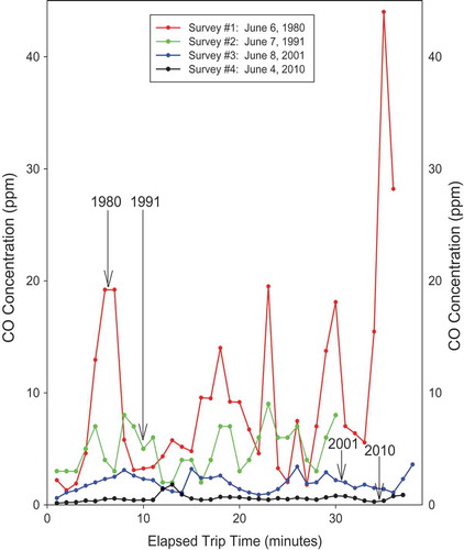
Our field data indicated that peak CO concentrations tend to occur at congested intersections, usually when cars accelerate after a traffic light turns from red to green. The probability of finding a “high-emitting” vehicle is greater at congested intersections than elsewhere on a highway, because the density of cars at congested intersections is larger. Thus, a small number of “high-emitting” cars at congested intersections could be the cause of the peaks in Figure 1. This result is consistent with the findings of a published paper by Ott, Switzer, and Willits (1994). They found (1) that those intersections on El Camino Real that had the highest “surrounding vehicle counts” showed the highest CO concentrations, and (2) that the highest CO concentrations were found in the “acceleration driving mode,” the next highest in the “stopped mode,” and the lowest in the “moving mode” of travel on the study site.

As shown in Figure 1, the reductions in typical and peak CO concentrations may be attributed to two policy decisions that affected mobile source emissions. One is California’s implementation of an inspection and maintenance (I/M) program (i.e., Smog Check) in 1984. I/M programs were implemented to identify vehicles that violated tailpipe exhaust emission standards and to ensure that their emission control systems were replaced or repaired. In an article published in em, Holmes and Cicerone wrote: “A general characterization is that approximately 10% of the fleet contributes 50% or more of the emissions of any single air pollutant” (2002, 16)

In theory, an effective I/M program could lower the rate of deterioration in fleet emissions over time. Hence, the maximum benefits of an I/M program would be achieved many years after it was adopted (Walsh 1999). Smog Check was implemented in 1984, about 7 yr before the start of the second field survey in 1991, 17 yr before the start of the third field survey in 2001, and 26 yr before the start of the fourth field survey in 2010. However, there were lingering criticisms of Smog Check’s effectiveness in the 1990s, which cast some doubt on this theory (Green 1998; U.S. Environmental Protection Agency 1995).

Another plausible explanation is that reductions in typical and peak CO concentrations occurred because tougher “durability standards” on emission controls were adopted by California in September 1990. These standards, which were phased in on new cars sold in California in 1993 and 1994, required automobile makers to extend warranties on emission control equipment from 5 yr or 50,000 miles to 10 yr or 100,000 miles. These “durability standards” were later incorporated by Congress as amendments to the Clean Air Act in November 1990 (Gordon 1991, 176–177).

Indicators of traffic conditions

In keeping with the “max-min-con” principle of our study design, we looked at whether reductions in CO exposure inside the test vehicle could be attributed to more favorable traffic conditions on the study site over the 30-yr period of the study. Instead, we found that three indicators of traffic conditions on the study site remained relatively steady during the 30-yr period of the study. These included averages in trip duration, trip speed, and the percentage of time spent at traffic lights (Table 5). In fact, reductions in exposure occurred despite an increase in the average number of motor vehicles surrounding the test vehicle at traffic signals. Table 5 shows that the average of this indicator varied from one survey to the next but ultimately increased by 28.2% between the first and last survey periods. This result could be explained by the fact that traffic engineers installed new signals at nine intersections and added left-hand turn lanes at existing signals to accommodate traffic growth between 1980 and 2010. The standard deviation and range of all indicators over time remained relatively constant. Thus, in-vehicle CO exposures fell over the 30-yr period of our study, even though three of the four traffic indicators remained relatively stable over that period, and the fourth indicator—surrounding vehicle count at traffic signals—increased during that period.

Table 5. Four traffic indicators by field survey.

Traffic indicator	Survey #1: 1980–1981	Survey #2: 1990–1991	Survey #3: 2001–2002	Survey #4: 2010–2011
Number of cases	50	50	50	50
Trip duration (min)
Mean ± 95% C.I.^a	39.6 ± 1.0	35.6 ± 1.2	38.9 ± 1.7	36.3 ± 1.5
SD	3.6	4.2	6.1	5.1
Range	31.2–48.0	29.0–49.0	26.9–53.2	29.6–53.0
Trip speed (mph)
Mean ± 95% C.I.^a	18.0 ± 0.5	20.2 ± 0.6	18.6 ± 0.8	19.9 ± 0.7
SD	1.7	2.2	2.8	2.6
Range	14.8–22.7	14.4–24.4	13.3–26.3	13.4–23.9
Percent of total trip time stopped at traffic lights
Mean ± 95% C.I.^a	27.4 ± 1.5	22.8 ± 1.8	29.4 ± 1.8	28.6 ± 1.8
SD	5.3	6.2	6.4	6.3
Range	17.0–42.2	11.6–41.0	17.7–42.2	19.5–46.9
Surrounding vehicle count at signalized intersections (vehicles)
Mean ± 95% C.I.^a	18.1 ± 1.8	20.9 ± 1.7	26.4 ± 2.1	23.2 ± 1.6
SD	6.3	6.1	7.4	5.7
Range	6.2–32.0	11.7–31.4	2.1–42.9	9.2–34.5

Notes. Source: Ott, Switzer, and Willits (1993) for Survey #1.

^aC.I. is the confidence interval.

The statistical rollback model

Although the survey means of the in-vehicle CO exposures are important, adverse health effects usually are associated with CO concentrations higher than the means. Hence, it is important to consider the full distribution of exposures on the highway. To evaluate the effect of controlling the full distribution of concentrations, Larsen (1961) proposed the “rollback” method to estimate how much source emission reduction is needed to achieve an ambient air quality standard. Ott (1995, 276–293) proposed a statistical theory of rollback (STR) utilizing Larsen’s lognormal model and applied it to CO concentrations measured inside the passenger compartment of a motor vehicle. This theory predicts that both the arithmetic mean and the standard deviation of the modeled frequency distribution of a year’s net CO exposure measurements on a highway will change in direct proportion to the expected value of the CO exhaust emission rates on the roadway. Therefore, if the average CO exhaust emission rates on the roadway decrease by a specific proportion, our hypothesis is that the arithmetic mean and the arithmetic standard deviation of the frequency distribution of net exposures will decrease by the same proportion. As a result, the coefficient of variation (ν), which is the ratio of the arithmetic standard deviation to the mean, will be fixed. If a lognormal probability model is fitted to the data, which often is justified by the observations, then the theoretical consequence of fixed ν is that the geometric standard deviation (σ_g) of the exposure distribution will be the same after emission control as before control, but the median will decrease in direct proportion to the degree of control. In the standard two-parameter lognormal model, the median is equal to the geometric mean.

This theory assumes that the CO trip means are affected by the random motion of air on the highway, which carries the emissions from vehicle tailpipes into the passenger compartments of motor vehicles traveling the roadway. This process occurs due to turbulence and mechanical mixing as pollutants are transported from tailpipes to the surrounding air and into nearby vehicles (Ott 1995; Yu, Hildemann, and Ott 1996). The arithmetic mean (expected value) of the exposures and the arithmetic standard deviation are assumed to be linearly related to the average emission rates on the roadway, while variability of the trip averages is attributed mainly to variation in traffic conditions and mechanical mixing. Thus, we hypothesize that the coefficient of variation (ν) of the frequency distributions of the net CO exposures for each year-long field survey will be approximately the same. In the lognormal model, the geometric standard deviation (σ_g) is related to the coefficient of variation (ν) as shown in eq 1:

(1) ${\sigma }_g=e^{\sqrt{\mathrm{l}\mathrm{n}\left({\nu }^2+1\right)}}$(1)

$\begin{array}{l}\text{where}{\sigma }_g=\text{geometric}\text{standard}\text{deviation}\text{and}\\ \text{}\nu =\text{coefficient}\text{of}\text{variation}.\end{array}$

Although the annual mean net exposure on the roadway may decrease due to reductions in emissions during each field survey, eq (1) of the statistical theory also predicts that the geometric standard deviation (σ_g) of the lognormal model representing the frequency distribution of net exposures will be fixed. For the four field surveys of CO measurements on El Camino Real, the coefficients of variation (ν) of the lognormal models that were fitted to the data were 0.3 in the first field survey, and 0.4 for each of the remaining three surveys (Table 6). Thus, the range of these coefficients was relatively small (from 0.3 to 0.4), which was consistent with the hypothesis that ν is approximately fixed over time. As a result, the slopes of the straight lines that were fitted to the cumulative CO frequency distributions of the four field surveys were approximately the same, despite the long time in years between the field surveys (Figure 2).

Table 6. Model parameters obtained by fitting the lognormal model to the net in-vehicle CO frequency distributions using linear regression.

Field survey	Arithmetic mean (ppm)	Arithmetic SD (ppm)	Coefficient of variation (ν)	Geometric mean (μg)^a(ppm)	Geometric SD (σg)	R^2
#1: 1980–1981	9.7	3.2	0.3	9.2	1.4	0.980
#2: 1991–1992	4.9	2.0	0.4	4.5	1.5	0.932
#3: 2001–2002	1.7	0.71	0.4	1.6	1.5	0.910
#4: 2010–2011	0.51	0.21	0.4	0.47	1.5	0.986

Note. ^a In the lognormal model, the geometric mean is equivalent to the median.

Figure 2. Logarithmic-probability plots of net in-vehicle CO concentrations for four field surveys.  The dots are the measured in-vehicle mean net CO trip concentrations on each field survey, including the outliers, and the straight lines are the lognormal models fitted to these data, along with their geometric means (μ_g) and their geometric standard deviations (σ_g).

To graphically compare the frequency distributions of the observed concentrations from the four field surveys, we sorted the 50 CO observations from each field survey in increasing order. Then we computed the plotting position of each data point as 100i/(n + 1) for i = 1, 2,…, n, where i is an index representing the order of each data point, and n is the total number of data points (i.e., n = 50 for each field survey). For each survey data set, we used Sigma-Plot Version 11 (Systat, Inc., San Jose, CA) to make a graph of the logarithm of the CO exposure to the base 10 on the vertical axis and the plotting position on the horizontal axis based on the integral of the normal (Gaussian) probability density function (Figure 2). On this type of graph, a frequency distribution that plots as a nearly straight line is approximately lognormal. A physical process has been suggested in the air pollution literature for the lognormal distribution (Ott 1990). Also, a great many observed pollutant concentration frequency distributions in the environment (e.g., outdoor air pollution, indoor air pollution, pollutants in streams, pollutants in the soil, pesticides in food) have been found to plot as straight lines on this type of graph (Ott 1995, 191–296).

We applied the Shapiro–Wilk test using Sigma-Plot Version 13 to the logarithm of the observed CO concentrations in each field survey. For Surveys #1 and #4, the results were consistent with the hypothesis at the p = 0.05 level of significance that the observations follow a lognormal distribution. Figure 2 shows that Surveys #2 and #3 had several outliers. When the two lowest CO concentrations were removed from Survey #2 and the lowest and two highest concentrations were removed from Survey #3, the lognormal hypothesis also could not be rejected at the p = 0.05 level of significance for these two surveys. For all four surveys, the results of the Shapiro–Wilk tests, the closeness of the observed data plotted in Figure 2 to the straight lines estimated from the models, and the relatively high R² values in Table 6 meet the criteria proposed by Larsen (1961) for air quality distributions that are approximately lognormal. In a lognormal distribution, the geometric standard deviation, which determines the slope of the line, is the ratio of the CO concentration at the 84.13th percentile to the CO concentration at the 50th percentile (the median). Despite these fixed slopes, the observed arithmetic mean net exposures showed a major decrease over the 30-yr period from 9.7 ppm to 4.8 ppm to 1.7 ppm to 0.5 ppm (Table 3), and these statistics agreed closely with the model parameters in Table 6.

We used regression analysis to find the slope and intercept of the straight-line fit to the frequency distribution on a logarithmic-probability graph. This analysis uses a least-squares calculation of the mean and standard deviation of the logarithms of the exposures. Because these results are plotted on a log₁₀ scale in Figure 2, we first must multiply the parameters of the lognormal model obtained from the Sigma-Plot software by log_e10, or ln(10), to obtain the basic mean and standard deviation of the logarithms. These results, in turn, are converted by standard formulas to the arithmetic and geometric model parameters, as listed in Table 6 and shown in Figure 2. The resulting geometric standard deviation of the model (σ_g), fitted to the data in this manner, was remarkably similar for the four field surveys: σ_g = 1.4 for Survey #1 and σ_g = 1.5 for Surveys #2, #3, and #4. These results were consistent with the second hypothesis of the rollback theory: The geometric standard deviation of the model was approximately the same for each year-long field survey.

Implications for protecting public health

The observed frequency distributions in Figure 2 are themselves useful for discussing the results of this study. In Survey #1, for example, the observed net arithmetic mean was 9.7 ppm, while the observed median net CO concentration was 9.2 ppm (Table 3). Thus, 50% of the trip means exceeded 9.2 ppm in 1980–1981. By comparison, only an estimated 4% of the CO trip averages exceeded 9 ppm during the 1991–1992 field survey just 10 yr later, a significant decrease that is relevant to protecting public health. The National Ambient Air Quality Standards for CO are 9 ppm for 8 hr and 35 ppm for 1 hr. Both standards, which are designed to protect human health throughout the United States, allow only one exceedance per year (U.S. Environmental Protection Agency 2018). The NAAQS were established by the Clean Air Act Amendments of 1970 (Ortolano 1997, 267–270).

By 1970, there were only a few in-vehicle CO exposure field studies. For example, the federal government used a van to measure exposure to CO in heavy traffic in 14 major U.S. cities between May 1966 and June 1967. Five of those cites were initially studied by Brice and Roesler (1966). Shortly thereafter, Lynn et al. (1967) remeasured those five cities and added nine more, for a total of 14 cities. These studies were performed about the same time that light-duty vehicle exhaust CO emission standards were adopted in the United States (Table 4). Although the in-vehicle CO measurements were not corrected for background levels, the overall average of the 20- to 30-min exposures on arterial highways was 22 ppm for 14 cities. About 10% of the 320 trips taken in these cities had in-vehicle CO averages above 33 ppm, with a maximum average of 60 ppm in Los Angeles and 61 ppm in Denver (U.S. Public Health Service 1970, 6–24, Tables 5 and 6).

By the time of our third field survey in 2001–2002, the observed net exposures on El Camino Real had dropped significantly: 94.6% of the net trip averages were less than 3 ppm, and 80% were less than 2 ppm. For example, Figure 2 shows that the 2-ppm data point for the 2001–2002 survey lies almost exactly on the vertical gridline showing an 80% cumulative percentage. In the 2010–2011 field survey, there was an even greater decrease in net CO trip exposures: 97% of the trip averages were estimated to be less than 1.0 ppm, with only 3% above 1.0 ppm. In that final field survey, Figure 2 shows that the observed data point at a cumulative frequency of 10% was 0.28 ppm and at 90% was 0.8 ppm. Therefore, subtracting 10% from 90% shows that 80% of the observed net CO exposures during the last field survey were in the narrow range between 0.28 and 0.8 ppm. This striking decrease over 30 yr is also evident in Figure 3, which shows a time-series plot of the mean net in-vehicle CO exposure computed from measurements for all 50 cases. As stated previously, each case consists of four matched trips—one selected from each field survey—to reduce the influence of variables related to traffic and weather conditions. Figures 2 and 3 both show the 50 net CO trip means for each field survey. The dots in Figure 2 are the ordered percentiles of the frequency distribution of the 50 trip means for each survey plotted on a logarithmic-probability graph, while the dots in Figure 3 are the same 50 trip means for each survey plotted as a time series.

Figure 3. A time-series plot of the mean net in-vehicle CO exposures for the 50 trips matched from each of the four field surveys of El Camino Real to reduce the influence of traffic and weather conditions.

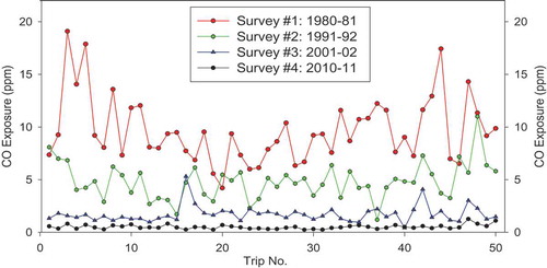
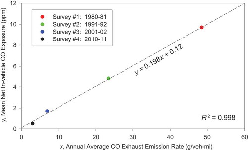
Overall, Table 3 shows a remarkable drop in the mean net CO concentration of each field survey of the highway over this 30-yr period. The drop in the mean was 50.5% between Surveys #1 and #2, 64.6% between Surveys #2 and #3, and 70.6% between Surveys #3 and #4. Thus, the overall mean net CO exposure decreased by at least 50% every decade. Finally, comparing the first and last field surveys, the overall mean net CO concentration on the highway decreased by 94.8% over all three decades. For the four field surveys, there also was evidence that the mean in-vehicle exposure was linearly related to the estimated annual average CO exhaust emission rate on the roadway, as indicated by the dashed straight line that was fitted to the observed means by linear regression (Figure 4). The mathematical expression of the regression model appears next to the dashed line in Figure 4. The statistics for this model indicated a strong fit to the data (F = 1073.5, p = 0.0009). Given only four sets of data, the CO exhaust emission rate showed a high degree of explanatory power (multiple R² = 0.998) in predicting the overall mean net CO exposure inside the vehicle. This finding of a linear relationship is consistent with the first hypothesis of the rollback theory. The next section explains how we estimated the annual average CO exhaust emission rate on the roadway for each field survey.

Figure 4. Mean net in-vehicle CO exposure measured on El Camino Real versus the annual average CO exhaust emission rates for four field surveys compared with dashed line fitted by linear regression.

CO exhaust emission rates

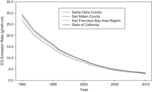
This section answers two important questions. First, are the CO exhaust emission rates on the El Camino Real study site, which connects Palo Alto in the northern part of Santa Clara County to Menlo Park in the southern part of San Mateo County, similar to those of other jurisdictions in California? To answer this question, we computed the VMT-weighted annual average CO running exhaust emission rates for the counties of Santa Clara and San Mateo, the San Francisco Bay Area Region, and the state of California using the 2011 EMFAC model (California Air Resources Board 2011). To use the EMFAC model, we had to assume that the estimated CO emission rates for a particular county (i.e., either San Mateo County or Santa Clara County) could be applied to the El Camino Real study site in the county, since the model did not give emission rates that were site-specific to a particular roadway. To run the model, we selected the “annual” option for season, the “2007” vehicle categories, the “aggregated” option for model years and speeds, and the “all” option for fuel. Figure 5 shows the CO exhaust emission rates for all four jurisdictions for the period from 1990 through 2010. It shows that the CO exhaust emission rates of the motor vehicle population of Santa Clara County, which holds about 78% of the El Camino Real study site, are slightly lower than, but still similar to, those of the other three jurisdictions: San Mateo County, the San Francisco Bay Area Region, and the state of California. This result suggests that the El Camino Real study site was representative of the San Francisco Bay Area Region and the state of California for the 20-yr period from 1990 to 2010.

Figure 5. VMT-weighted average CO running exhaust emission rates for Santa Clara and San Mateo counties, the San Francisco Bay Area Region, and the state of California for the 1990 to 2010 period.

Second, do the measured reductions in passenger CO exposures on the study site correspond to reductions in CO exhaust emission rates for San Mateo and Santa Clara counties over the 30-yr period of the study? To answer this question, we developed second-order and third-order polynomial regression models to estimate the VMT-weighted average CO running exhaust emission rates for 1980 for both San Mateo County and Santa Clara County. These models were calibrated using data generated by the 2011 EMFAC model for each county and for each year of the 1990 through 2010 period (California Air Resources Board 2011). The data for these regression models included the precontrol exhaust emission rate of 84.0 g/veh-mi for 1965 as reported in the literature (Godish 2004, 280). The 1980 emission rates for these two counties were unknown, because they could not be estimated directly by the 2011 EMFAC model. Yet the 1980 CO exhaust emission rate of each county was very important, because the 1980–1981 field survey served as the baseline for estimating reductions in CO exposure for subsequent survey periods. The coefficient of determination for each regression model was very high (R² > 0.99) and the F statistic for each model was also satisfactory (p < 0.00001). Table 7 shows the mean net in-vehicle CO concentration for the four survey periods along with the VMT-weighted average CO running exhaust emission rates for both San Mateo and Santa Clara counties, as estimated by the second- and third-order polynomial regression models. Table 7 also shows that the percentage reductions in both the in-vehicle CO concentrations and the CO exhaust emission rates for each county and survey period relative to those of 1980 are very similar for each model.

Table 7. In-vehicle CO concentrations and the estimated annual average CO exhaust emission rates by county and survey period.

			Second-order polynomial model		Third-order polynomial model
Survey period	Mean net in-vehicle  CO concentration for study site^a (ppm)	Percentage reduction relative to 1980–1981	Average CO exhaust emission rate (g/mile)	Percentage reduction relative to 1980	Average CO exhaust emission rate (g/mile)	Percentage reduction relative to 1980
San Mateo County
1980–1981	9.7		44.4		51.9
1991–1992	4.8	50.5	23.4	47.3	23.4	54.9
2001–2002	1.7	82.5	6.9	84.5	6.9	86.7
2010–2011	0.5	94.8	3.0	93.2	3.0	94.2
Santa Clara County
1980–1981	9.7		42.6		48.5
1991–1992	4.8	50.5	23.4	45.1	23.4	51.8
2001–2002	1.7	82.5	6.9	83.8	6.9	85.8
2010–2011	0.5	94.8	3.0	93.0	3.0	93.8

Note. ^aThe means are identical for each county, because the study site spans a portion of each county and the net in-vehicle CO concentration in the table represents the mean value for the entire trip on the study site.

The annual average CO exhaust emission rate (g/veh-mi) in Figure 4 was based on the data shown for the third-order polynomial model for Santa Clara County in Table 7. Santa Clara County was chosen because 78% of each trip on the study site occurred in that county. The third-order polynomial model was chosen because it provided the best fit to the emission rate data generated by the EMFAC model (F = 3452.9, p < 0.00001) to estimate the 1980 emission rate, and it had very good explanatory power (adjusted R² = 0.998). Also, that model’s estimate of the percentage reduction in CO emissions for each field survey, relative to the baseline CO emission rate in 1980, was very similar to the percentage reduction in CO exposure for each field survey relative to the first survey in 1980–1981.

Ambient CO concentrations

The nearest ambient CO fixed-site monitor was located at 897 Barron Ave. in Redwood City, CA, or about 5.2 miles from the midpoint of each trip, which was the intersection of El Camino Real and Page Mill Rd. The Bay Area Air Quality Management District did not monitor CO concentrations near roads in Santa Clara County until 2014, 3 yr after we completed collection of passenger exposure data on the El Camino Real study site (Bay Area Air Quality Management District 2015, 37). The average of the hourly ambient CO concentrations that corresponded to the dates and trip starting times of field surveys was 1.30 ppm for Survey #1, 1.31 ppm for Survey #2, 0.61 ppm for Survey #3, and 0.41 ppm for Survey #4 (Table 8). The ratio between the mean net in-vehicle CO concentration and the mean hourly ambient CO concentration fell from 7.5 for the 1980–1981 survey period to 1.2 for the 2010–2011 period. This result supports the theory that the in-vehicle CO concentrations, which primarily depend on the CO emissions from vehicles on the roadway, would show a greater decrease in value than would the ambient CO concentrations, given that the latter are affected more by the collective CO emissions of sources in the entire community than by the CO emissions on a single roadway. The data shown in Table 8 also indicate that ambient CO concentrations, as measured at the nearest fixed site monitor to our study site, did not represent in-vehicle CO exposures on the study site during the first survey in 1980–1981. However, this monitor appeared to give a better representation of in-vehicle CO exposures on the study site by the fourth survey in 2010–2011.

Table 8. Ambient CO concentrations (ppm) at nearest fixed site monitor by field survey^a.

	Survey #1: 1980–1981	Survey #2: 1990–1991	Survey #3: 2001–2002	Survey #4: 2010–2011
Monitor precision	1.0	1.0/0.1^b	0.1	0.1
Hourly CO concentration during field surveys
Average	1.30	1.31	0.61	0.41
SD	0.55	0.57	0.36	0.27
Range	1–3	0.7–4.2	0.3–2.0	0.2–2.0
Number of observations	46	49	46	48

Notes. Sources: California Air Quality Data—Selected data available for download.

http://www.arb.ca.gov/aqd/aqdcd/aqdcddld.htm for 1980–81 survey period (accessed July 2002). https://www.arb.ca.gov/aqmis2/display.php?report=SITE31D&site=2125&year=2017&mon=09&day=11&hours=all&statistic=HVAL&ptype=aqd&param=CO for 1990–91, 2001–02 and 2010–11 survey periods (accessed June 2012). Personal communication with James Cordova, Air Quality Meteorologist, Bay Area Air Quality Management District, July 2002, for 1991–1992 and 2001–2002 survey periods.

^aThe intersection of El Camino Real and Page Mill Road was the midpoint of the study site.

^bThe Bay Area AQMD reported that the precision of the monitor improved from 1 ppm to 0.1 ppm starting January 1, 1991.

Conclusion

The results of this study, which is based on four similar field surveys, each one approximately 10 yr apart, show that the California motor vehicle emission control program has been very effective in reducing in-vehicle exposure to CO in traffic between 1980 and 2010. The federal CO exhaust emission standards for new passenger cars have been nearly identical to the California standards since 1980. Thus, it appears likely that CO exposures on highways elsewhere in the United States have experienced a similar decline, especially if they have vehicle inspection and maintenance programs similar to those in California.

Measurement of in-vehicle CO exposure is useful for assessing the effectiveness of emission control systems on mobile sources, particularly if these systems are implemented over a long period of time to comply with progressively tighter emission standards. Exposure measurements can supplement measurements of ambient air quality at fixed-site monitors, particularly in locations where monitors may not be representative of personal CO exposure. Overall, the average CO exposures on the El Camino Real study site changed drastically over time in response to emission control efforts. These efforts reduced exposures by 50.5% in the first decade, 82.5% over the first two decades, and 94.8% over the full 30 yr of the study.

What was particularly striking were the similarities in the forms of the frequency distributions of the CO trip averages for each of the four field surveys. Despite the major decrease of nearly 95% in the mean net CO concentrations inside the test vehicle on the roadway over 30 yr, the geometric standard deviations of the frequency distributions of the four field surveys were about the same. This finding gives support to the second hypothesis of the rollback theory, that one can predict the frequency distribution of an entire year of highway exposure observations by knowing the geometric standard deviation and the mean for that year. As we have shown, such predictions include not only typical exposures, but also the higher exposures occurring less often in traffic over the year, such as concentrations observed at the expected highest 10% or even the highest 5% of exposures. Equally important is the finding that the relationship between the mean net CO exposure observed on the roadway and the estimated average CO emission rate is essentially linear, which gives support to the first hypothesis of the rollback theory.

Periodic measurements of in-vehicle exposure to air pollution using a standard protocol can be a useful supplementary tool for assessing the effectiveness of emission control programs. Such measurements have been used in studies of in-vehicle exposure to ultrafine particles (Zhu et al. 2007). The methodology of in-vehicle exposure studies is relatively easy to apply. Such studies also provide data that are directly relevant to protecting public health at modest cost.

Many developing countries launched or expanded their mobile source emission control programs in the 1990s (Faiz, Weaver, and Walsh 1996; Health Effects Institute 2004), yet many of them do not have adequate inspection and maintenance (I/M) programs (Freeman et al. 2015). While several in-vehicle exposure studies have been completed in China, India, and Indonesia, very few studies of this type have been done elsewhere in Asia, according to Han and Naeher (2006), and none of them have been repeated on a periodic basis to establish trends as far as we know. Consequently, such countries could use the methods of the El Camino Real study to establish baseline information on in-vehicle exposure and periodically remeasure exposure using a standard data collection protocol to assess progress and facilitate comparisons over time. Ideally, the measurement protocol should take advantage of modern personal monitors, follow good quality assurance procedures, represent typical travel patterns, account for background concentrations, and recognize that exposure can vary over time and space.

Acknowledgments and Disclaimer

The authors gratefully acknowledge the assistance of Professor Paul Switzer and Dr. Neil Willits, who were previously affiliated with the Department of Statistics at Stanford University. They assisted Dr. Wayne Ott in collecting, processing and analyzing data during the first survey period in 1980–1981. That work received partial funding from the U.S. Environmental Protection Agency (EPA) under Cooperative Agreement CR814694 to the Societal Institute for the Mathematical Sciences (SIMS) and to Stanford University. Although the U.S. EPA reviewed and approved that work, this paper may not necessarily reflect its views and no official endorsement should be inferred. Moreover, mention of trade names or commercial products in the paper does not constitute endorsement or recommendation for use. Finally, the authors are grateful to Dr. Douglas Eisinger of SonomaTech in Petaluma, CA. He provided advice to Professor Peter Flachsbart on the use of the EMFAC model to generate CO running exhaust emission rates. We also thank three anonymous reviewers for their insightful comments and suggestions on a previous version of our paper.

Additional information

Funding

This work was supported by the U.S. Environmental Protection Agency (Cooperative Agreement CR814694).

Notes on contributors

Peter Flachsbart

Peter Flachsbart is an associate professor in the Department of Urban and Regional Planning, University of Hawaii at Manoa, Honolulu, HI.

Wayne Ott

Wayne Ott is an adjunct associate professor in the Department of Civil and Environmental Engineering at Stanford University, Stanford, CA.

References

- Akland, G., T. Hartwell, T. Johnson, and R. Whitmore. 1985. Monitoring human exposure to carbon monoxide in Washington, D.C., and Denver, Colorado, during the winter of 1982–1983. Environ. Sci. Technol. 19:911–18. doi:10.1021/es00140a004.
- Alexis, A., A. Delao, C. Garcia, M. Nystrom, and K. Rosenkranz. 2001. The California almanac of emissions and air quality. 2001 ed. Sacramento: Planning and Technical Support Division, California Air Resources Board.
- Bay Area Air Quality Management District. 2015. 2014 air monitoring network plan. San Francisco: Bay Area Air Quality Management District. July 1.
- Brice, R. M., and J. F. Roesler. 1966. The exposure to carbon monoxide of occupants of vehicles moving in heavy traffic. J. Air Pollut. Control Assoc. 16:597–600.
- California Air Resources Board. 1997. California exhaust emission standards and test procedures for 1988 and subsequent model passenger cars, light-duty trucks, and medium-duty vehicles. Sacramento: Air Resources Board.
- California Air Resources Board. 2011. EMFAC2011: Technical documentation. Sacramento: Air Resources Board.
- California Department of Transportation. 2017. www.dot.ca.gov/hq/traffops/saferesr/trafdata ( accessed July 5, 2017).
- Cox, P., A. Delao, and A. Komorniczak. 2013. The California almanac of emissions and air quality. 2013 ed. Sacramento: Air Quality Planning and Science Division, California Air Resources Board.
- Cox, P., A. Delao, A. Komorniczak, and R. Weller. 2007. The California almanac of emissions and air quality. 2007 ed. Sacramento: Air Quality Planning and Science Division, California Air Resources Board.
- de Nazelle, A., O. Bode, and J. P. Orjuela. 2017. Comparison of air pollution exposures in active vs. passive travel modes in European cities: A quantitative review. Environ. Int 99:151–60. doi:10.1016/j.envint.2016.12.023.
- Duan, N. 1982. Models for human exposure to air pollution. Environ. Int. 8:305–09. doi:10.1016/0160-4120(82)90041-1.
- Eisinger, D. S. 2010. Smog check: Science, federalism, and the politics of clean air. Washington, D.C.: RFF Press.
- El-Fadel, M., and L. Abi-Esber. 2009. In-vehicle exposure to carbon monoxide emissions from vehicular exhaust: A critical review. Crit. Rev. Environ. Sci. Technol. 39:585–621. doi:10.1080/10643380701798264.
- Faiz, A., C. Weaver, and M. Walsh. 1996. Air pollution from motor vehicles: Standards and technologies for controlling emissions. Washington, D.C.: The International Bank for Reconstruction and Development/The World Bank.
- Flachsbart, P. G. 1995. Long-term trends in United States highway emissions, ambient concentrations, and in-vehicle exposure to carbon monoxide in traffic. J. Expo. Anal. Environ. Epidemiol. 5:473–95. https://www.ncbi.nlm.nih.gov/pubmed/8938245.
- Flachsbart, P. G. 1999. Human exposure to carbon monoxide from mobile sources. Chemosphere–Global Change Sci. 1 (103):301–29. doi:10.1016/S1465-9972(99)00030-6.
- Flachsbart, P. G. 2007. Chapter 6: Exposure to carbon monoxide. In Exposure analysis ed. W. R. Ott, A. C. Steinemann, and L. A. Wallace, 113-46. Boca Raton, FL: CRC Taylor & Francis.
- Freeman, B., F. Gharabaghi, S. Faisal, M. Abdullah, and J. Thé. 2015. Vehicle I/M programs for developing nations. em: the magazine for environmental managers, April 14–18.
- Godish, T. 2004. Air quality. 4th ed. Boca Raton, FL: Lewis Publishers, CRC Press.
- Gordon, D. 1991. Steering a new course: Transportation, energy, and the environment. Washington, D.C.: Island Press.
- Green, K. 1998. Checking up on smog-check: A critique of traditional inspection and maintenance programs. In Proceedings of the A&WMA’s 91st Annual Meeting and Exhibition, San Diego, CA, June 14–18. Paper 98-TA4C.01 (A717).
- Han, X., and L. P. Naeher. 2006. A review of traffic-related air pollution exposure assessment studies in the developing world. Environ. Int. 32:106–20. doi:10.1016/j.envint.2005.05.020.
- Health Effects Institute. 2004. Health effects of outdoor air pollution in developing countries of Asia: A literature review. Special Report 15, Health Effects Institute, Boston.
- Holmes, K., and R. Cicerone. 2002. The road ahead for vehicle emissions inspection and maintenance programs. em: the magazine for environmental managers, July 15–22.
- Johnson, J. H. 1988. Automotive emissions. In Air pollution, the automobile, and public health, ed. A. Y. Watson, R. R. Bates, and D. Kennedy, 39–76. Washington, D.C: National Academy Press.
- Kerlinger, F. N. 1986. Foundations of behavioral research. New York: Holt, Rinehart and Winston.
- Kyutoku, R. 2002. Office of Operations, District 4, Caltrans, Oakland, CA. Personal communication July.
- Langan, L. 2006. Langan model T15n carbon monoxide measurer. San Francisco, CA: Langan Products, Inc. Accessed October 16, 2018. http://www.langan.biz/man_soft_files/T15n_Manual.pdf.
- Larsen, R. I. 1961. A method for determining source reduction required to meet air quality standards. J. Air Pollut. Control Assoc. 11:71–76.
- Lynn, D., E. Tabor, W. Ott, and R. Smith. 1967. Present and future commuter exposure to carbon monoxide. In Proceedings of the 60th Annual Meeting of the Air Pollution Control Association, Cleveland, OH, June. Paper 67-5.
- National Research Council. 2003. Managing carbon monoxide pollution in meteorological and topographical problem areas. Washington, D.C.: The National Academies Press.
- Ortolano, L. 1997. Environmental regulation and impact assessment. New York: John Wiley & Sons.
- Ott, W., H. Vreman, P. Switzer, and D. Stevenson. 1995. Evaluation of electrochemical monitors for measuring carbon monoxide concentrations in indoor, in-transit, and outdoor microenvironments. In Proceedings of the International Symposium, Measurement of Toxic and Related Air Pollutants, May 16–18. Research Triangle Park, NC. Environmental Protection Agency and Air & Waste Management Association. Paper VIP-50, 172–77. Accessed September 30, 2018. https://www.researchgate.net/publication/320826839.
- Ott, W., N. Klepeis, and P. Switzer. 2008. Air change rates of motor vehicles and in-vehicle pollutant concentrations from secondhand smoke. J. Expo. Sci. Environ. Epidemiol. 18:312–25. doi:10.1038/sj.jes.7500601.
- Ott, W., P. Switzer, and N. Willits. 1993. Carbon monoxide exposures inside an automobile traveling on an urban arterial highway: Final Report on the 1980–81 field study. SIMS Technical Report No. 150, Department of Statistics, Stanford University, Stanford, CA. Accessed September 30, 2018. https://www.researchgate.net/publication/244988959.
- Ott, W., P. Switzer, and N. Willits. 1994. Carbon monoxide exposures inside an automobile traveling on an urban arterial highway. J. Air Waste Manage. Assoc. 44:1010–18. doi:10.1080/10473289.1994.10467295.
- Ott, W. R. 1990. A physical explanation of the lognormality of pollutant concentrations. J. Air Waste Manage. Assoc. 40:1378–83. doi:10.1080/10473289.1990.10466789.
- Ott, W. R. 1993. Trends of in-vehicle CO exposures on a California arterial highway over one decade. In Proceedings of A&WMA’s 86th Annual Meeting & Exhibition, Denver, CO, June 14–18. Paper No 93-RP-116B.
- Ott, W. R. 1995. Environmental statistics and data analysis. Boca Raton, FL: Lewis Publishers, CRC Press.
- Privitera, G. J. 2012. Statistics for the behavioral sciences. Los Angeles: Sage Publications.
- Rodes, C., L. Sheldon, D. Whitaker, A. Clayton, K. Fitzgerald, J. Flanagan, F. DiGenova, S. Hering, and C. Frazier. 1998. Measuring concentrations of selected air pollutants inside California vehicles [final report]. Contract No. 95–339, California Environmental Protection Agency, Air Resources Board, Sacramento.
- Roscoe, J. T. 1975. Fundamental research statistics for the behavioral sciences. 2nd ed. New York: Holt, Rinehart and Winston.
- Tashakkori, A., and C. Teddlie. 1998. Mixed methodology: Combining qualitative and quantitative approaches. Thousand Oaks, CA: Sage Publications.
- U.S. Department of Transportation. 1999. Transportation and air quality: Selected facts and figures. Washington, D.C.: Federal Highway Administration.
- U.S. Environmental Protection Agency. 1995. EPA I/M briefing book: Everything you ever wanted to know about inspection and maintenance. EPA-AA-EPSD-IM-94-1226, Office of Air and Radiation, Washington, D.C..
- U.S. Environmental Protection Agency. 2000. Air quality criteria for carbon monoxide. Final Report. EPA 600/P-99/001F, Office of Research and Development, National Center for Environmental Assessment, Washington, D.C.
- U.S. Environmental Protection Agency. 2010. Integrated science assessment for carbon monoxide. EPA 600/R-09-019F, Office of Research and Development, National Center for Environmental Assessment—RTP Division, Research Triangle Park, NC.
- U.S. Environmental Protection Agency. 2017. National air quality: Status and trends of key air pollutants. Washington, D.C: U.S. Environmental Protection Agency. Accessed September 30, 2018. https://gispub.epa.gov/air/trendsreport/2017/.
- U.S. Environmental Protection Agency. 2018. NAAQS table. Accessed September 30, 2018. https://www.epa.gov/criteria-air-pollutants/naaqs-table.
- U.S. Public Health Service. 1970. Air quality criteria for carbon monoxide, Final Report. National Air Pollution Control Administration Publication No. AP-62, U.S. Department of Health, Education, and Welfare, Washington, D.C.
- Walsh, M. P. 1999. Chapter 5: Motor vehicle emission control measures. In Urban traffic pollution, ed. D. Schwela and O. Zali, 133-74. London: E & FN Spon.
- Xu, B., C. Xiaokai, and J. Xiong. 2018. Air quality inside motor vehicles’ cabins: A review. Indoor Built Environ. 27:452–65. doi:10.1177/1420326X16679217/journals.sagepub.com/home/ibe.
- Yu, L., L. Hildemann, and W. Ott. 1996. A mathematical model for predicting trends in carbon monoxide emissions and exposures on urban arterial highways. J. Air Waste Manage. Assoc. 46:430–40. doi:10.1080/10473289.1996.10467476.
- Zhu, Y., A. Eiguren-Fernandez, W. C. Hinds, and A. H. Miguel. 2007. In-cabin commuter exposure to ultrafine particles on Los Angeles freeways. Environ. Sci. Technol. 41:2138–45. doi:10.1021/es0618797.