Spatial differences in ambient coarse and fine particles in the Monterrey metropolitan area, Mexico: Implications for source contribution

ABSTRACT

The ambient air of the Monterrey Metropolitan Area (MMA) in Mexico frequently exhibits high levels of PM₁₀ and PM_2.5. However, no information exists on the chemical composition of coarse particles (PM_c = PM₁₀ – PM_2.5). A monitoring campaign was conducted during the summer of 2015, during which 24-hr average PM₁₀ and PM_2.5 samples were collected using high-volume filter-based instruments to chemically characterize the fine and coarse fractions of the PM. The collected samples were analyzed for anions (Cl^–, NO₃^–, SO₄^2–), cations (Na⁺, NH₄⁺, K⁺), organic carbon (OC), elemental carbon (EC), and 35 trace elements (Al to Pb). During the campaign, the average PM_2.5 concentrations did not showed significance differences among sampling sites, whereas the average PM_c concentrations did. In addition, the PM_c accounted for 75% to 90% of the PM₁₀ across the MMA. The average contribution of the main chemical species to the total mass indicated that geological material including Ca, Fe, Si, and Al (45%) and sulfates (11%) were the principal components of PM_c, whereas sulfates (54%) and organic matter (30%) were the principal components of PM_2.5. The OC-to-EC ratio for PM_c ranged from 4.4 to 13, whereas that for PM_2.5 ranged from 3.97 to 6.08. The estimated contribution of Secondary Organic Aerosol (SOA) to the total mass of organic aerosol in PM_2.5 was estimated to be around 70–80%; for PM_c, the contribution was lower (20–50%). The enrichment factors (EF) for most of the trace elements exhibited high values for PM_2.5 (EF: 10–1000) and low values for PM_c (EF: 1–10). Given the high contribution of crustal elements and the high values of EFs, PM_c is heavily influenced by soil resuspension and PM_2.5 by anthropogenic sources. Finally, the airborne particles found in the eastern region of the MMA were chemically distinguishable from those in its western region.

Implications: Concentration and chemical composition patterns of fine and coarse particles can vary significantly across the MMA. Public policy solutions have to be built based on these observations. There is clear evidence that the spatial variations in the MMA’s coarse fractions are influenced by clearly recognizable primary emission sources, while fine particles exhibit a homogeneous concentration field and a clear spatial pattern of increasing secondary contributions. Important reductions in the coarse fraction can come from primary particles’ emission controls; for fine particles, control of gaseous precursors—particularly sulfur-containing species and organic compounds—should be considered.

Introduction

Population exposure to PM₁₀ (particles with an aerodynamic diameter less than 10 μm) and PM_2.5 (fine particles with an aerodynamic diameter less than 2.5 μm) has been associated with cardiovascular and respiratory diseases, as well as other human health impacts, worldwide (Davidson, Phalen, and Solomon 2005; Grahame, Klemm, and Schlesinger 2014; Lippmann 2011; Pope et al. 2011). The World Health Organization (WHO) has set recommended air quality standards for PM₁₀ at 50 µg m^–3 for 24-hr averages and 20 µg m^–3 for annual averages; for PM_2.5, these standards are set to 25 µg m^–3 for 24-hr averages and 10 µg m^–3 for annual ones (WHO, 2006).

PM₁₀ mass concentrations in ambient air are categorized primarily into two size fractions: PM_c (coarse particles with an aerodynamic diameter between 2.5 and 10 μm) and PM_2.5. The sum of these two fractions is PM₁₀. Several studies have focused on the health effects of PM_2.5, as they have been linked to adverse human health effects (Ito et al. 2011; Ostro et al. 2008). However, cardiovascular and respiratory effects, as well as total mortality, have also been associated with PM_c (Atkinson et al. 2010; Chen et al. 2011; Graff et al. 2009; Mallone et al. 2011; Meister, Johansson, and Forsberg 2012; Tobías et al. 2011), which has implications for environments where PM_c are often the major fraction (50–70%) of PM₁₀ (Clements et al. 2013; Sprovieri et al. 2011; Sprovieri and Pirrone 2008). This is relevant for the Monterrey Metropolitan Area (MMA), a region with a semiarid climate that could suggest a relevant contribution of geological material (Al, Ca, Si, and Fe) to PM_c.

Airborne particles are a complex mixture of carbonaceous material, soluble inorganic compounds, and trace elements. In addition, each size fraction has a characteristic chemical profile. The chemical composition of airborne particles is a key factor for determining their source contributions. Based on the size fraction, possible sources of PM_2.5 include emissions from anthropogenic-related activities, such as transportation, electricity generation, biomass burning, and industrial activities; natural sources, such as vegetative detritus; and secondary formation processes, including nucleation and growth by photochemical processes (George and Abbatt 2010; Seinfeld and Pandis 2006; Zhang et al. 2012). In contrast, PM_c commonly come from abrasion processes, including crustal material and vehicle wear products (Minguillón et al. 2012; Richard et al. 2011). Other sources of PM_c include animal feeding operations and handling operations for bulk material, such as grain processing (Cambra-Lopez et al. 2010). Primary and secondary aerosols undergo chemical and physical aging processes in the atmosphere that affect the contribution to PM_2.5 and PM_c of the different chemical species (Jimenez et al. 2009).

In the MMA, the third largest urban center in Mexico, air pollution attributable to airborne particles has become a significant problem for both visibility and human health. In 2015, the MMA exhibited annual averages in its routine monitoring network in the range of 20–34 μg m^–3 for PM_2.5 and 46–84 μg m^–3 for PM₁₀; these values exceeded their corresponding national air quality standards of 12 μg m^–3 and 40 μg m^–3, respectively. Only in the previous year, 24-hr average standards were exceeded up to 18 days (PM_2.5) and 191 days (PM₁₀) in comparison with other pollutants, for example ozone, that exceeded their 1-hr standard up to 53 days. As in other parts of the world, in Mexico, high levels of suspended particulate matter in the ambient air have been associated with health risks, neonatal mortality, and visits to hospitals (Hinojosa-Velasco et al. 2010; Mejía-Velázquez and Lerma-Serna 2013; Rojas-Moreno et al. 2008). In the MMA, several studies have been conducted to chemically characterize the ambient PM_2.5 and PM₁₀ (Badillo-Castañeda et al. 2015; Blanco-Jiménez et al. 2015; Garza-Ocañas et al. 2010; González et al. 2016; González Cárdenas 2014; Mancilla et al. 2016; Martínez et al. 2012), and other studies have used these chemical characterizations to carry out source apportionment calculations (Mancilla et al. 2016; Martínez et al. 2012) and develop chemical emission profiles for PM_2.5 (Mancilla, Araizaga, and Mendoza 2012; Mancilla and Mendoza 2012; Medina Gaitán 2015; Valdez Cerda et al. 2011). However, many of these studies have focused on PM_2.5; only Blanco-Jiménez et al. (2015) estimated a preliminary source contribution for PM_c.

Because airborne particles are strongly linked to air pollution in the MMA, it is advisable to investigate their components and emission sources for both coarse and fine size fractions. These data are key both to assessing the efficacy of public policies and programs designed to reduce air pollution and to updating and improving them. Unlike previous studies, the present study simultaneously analyzes the chemical composition of particles in the fine and coarse fractions in several urban locations within the MMA. In addition, the secondary organic aerosol (SOA) contributions and enrichment factors (EF) are estimated to identify the origin of the fine and coarse particles. This analysis will provide new data to support decision making about air quality in the MMA.

Methodology

Sampling site

The MMA is the third largest Mexican urban center and is located in the northeastern region of the country (25°40’17” N, 100°18’31” W). It has 5.1 million inhabitants (INEGI 2015), encompasses 6,682 km² (SEDESOL et al. 2007), and has 1.9 million vehicles (INEGI 2015). It has a local routine monitoring network (Integral Environmental Monitoring System, with initials SIMA in Spanish) that monitors the air quality of the airshed. Prior to this study, SIMA had seven operational monitoring stations spread throughout the MMA. Data from SIMA were used to determine the sampling sites through the comparison of PM_2.5 and PM₁₀ concentrations among monitoring stations. These sampling sites were selected by performing an analysis based on coefficients of divergence (COD) using the recorded ambient concentrations of PM_2.5 from five air monitoring stations and PM₁₀ from seven. Data from only five stations were used for fine PM because these were the only stations that had operational PM_2.5 equipment with valid registries. Annual CODs were determined for each monitoring station in relation to the others for the period from 2011 to 2014 using the following equation (Pinto, Lefohn, and Shadwick 2004):

(1) $CO{D}_{jk}=\sqrt{\frac{1}{p}\sum _{i=1}^p{\left[\frac{x_{ij}-x_{ik}}{x_{ij}+x_{ik}}\right]}^2}$(1)

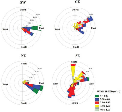
where x_ij and x_ik represent the 24-hr average concentration of either PM_2.5 or PM₁₀ for the observation i at the j and k monitoring stations, and p is the total number of observations to be compared. A COD_jk value of 0 implies that the observations for a given pair of monitoring stations are alike, whereas a value of 1 means that the values obtained by the monitoring stations are completely dissimilar. In this study, the monitoring stations with the highest COD values were selected as sampling sites in order to analyze the spatial variability of the air pollutant concentrations across the MMA. The annual CODs for each monitoring station were determined for four years (2011–2014), conducting a matrix comparison of those values. Subsequently, the calculated CODs for each monitoring station for each of the four years were added. Finally, the selection of the sampling sites was based on the highest sum of CODs. These results are summarized in Table 1. As can be observed, during 2011–2014, the station located in the northwest exhibited the lowest sum of CODs. Therefore, for both PM_2.5 and PM₁₀, the selected sampling sites were the southwest (SW), downtown (CE), northeast (NE), and southeast (SE) monitoring stations (Figure 1). The SW site is located downwind of most of the emission sources in the MMA, and it is where the highest concentrations of some pollutants, such as PM₁₀ and ozone, regularly occur. The CE site allows the assessment of the mix of pollutants that are emitted from area and mobile sources in the downtown area of the MMA and the influence of downwind sources to the east. Finally, the NE site is located downwind from an industrial corridor, and the SE sites are downwind from limited industrial areas; both areas are densely populated. Figure 2 depicts the predominant direction of wind flow across the MMA during the monitoring campaign (east to west, with some variations); the east-to-west wind direction is the typical pattern for the MMA (Hernández Paniagua, Clemitshaw, and Mendoza 2017). This information illustrates the downwind direction for each site, as described earlier, and is key to understanding the enrichment processes of the coarse and fine particle fractions.

Table 1. Sum of CODs for PM_2.5 and PM₁₀ in the MMA.

Station/year	2011		2012		2013		2014
	PM2.5	PM10	PM2.5	PM10	PM2.5	PM10	PM2.5	PM10
SE	0.94	0.95	0.70	0.87	0.67	1.16	0.75	1.34
NE	0.66	0.86	0.64	0.74	0.68	1.05	0.65	1.07
CE	0.63	0.98	0.59	1.09	0.64	1.40	0.60	1.05
NW	0.65	0.89	0.54	0.76	0.55	1.07	0.59	0.98
SW	0.72	1.07	0.68	*	0.67	1.13	0.63	1.24
NW2	*	1.26	*	1.06	*	1.40	*	1.15
N	*	1.04	*	0.83	*	1.14	*

Notes. NW = Northwest; NW = Northwest 2; N = North.

*No data were available to calculate the corresponding COD.

Figure 1. Location of all monitoring stations in the MMA, with sampling sites (red circles) and nonsampling sites (gray circles) for PM_2.5 and PM_c.

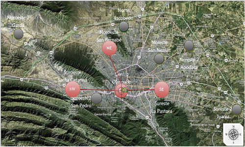
Figure 2. Wind rose diagrams for all sampling sites in the MMA.

Sampling periods and equipment

Particle samples were collected on 8 × 10-inch (Whatman QMA) quartz microfiber filters using two high-volume filter-based samplers (Tisch Environmental, Inc.) operated at a flow rate of 1.13 m³ min^–1 and located side by side, one with a size-selective inlet for PM_2.5 (model TE-6001–2.5) and the other with a size-selective inlet for PM₁₀. The calibration of the samplers was performed before the start of the sampling at each site, using its corresponding calibration orifice (National Institute Standards and Technology Traceable Calibration Certificate). In addition, the impactor stages were greased before sampling at each location using a silicone oil release spray (Dow Corning). At each sampling site, 24-hr averaged PM_2.5 and PM₁₀ samples were collected for 7 days. The samples were collected at each sampling site during different periods, as follows: June 3 to June 9 (SW), June 11 to June 15 and June 25 to June 26 (CE), June 29 to July 5 (NE), and July 7 to July 14 (SE). Although the samples were not collected simultaneously, the sampling was conducted during the same season; this allows us to explore spatial differences across the MMA. For each sample, the collection started every day at 8:00 a.m. and ended at 8:00 a.m. of the next day. In total, 56 samples and 4 field blanks were collected for this monitoring campaign. For each field blank, the filter was installed and left in the sampler, with the sampler turned off, for 24 hr; the filter was treated in the same way as the loaded filters during all transportation and storage stages. These blanks were used to correct each ambient sample. In addition, all the samples were stored in a freezer at –20°C until they were analyzed in September 2015.

Analyses and chemical characterization

The analytical measurements were conducted according to the letter of each standard method described in this section. The microfiber quartz filters were baked at ~600°C for at least 8 hr in order to remove organic residues prior to use in the field. The filters were weighed before and after field sampling using a Sartorius ME5 microbalance (1 mg readability) in a weighing chamber with controlled temperature and relative humidity to obtain the total collected particulate matter. The allowable weighing temperature was a 24-hr average between 20°C and 23°C (standard deviation less than 2°C), and the 24-hr mean relative humidity was maintained between 30% and 40% (standard deviation less than 5%). The same filters were then analyzed for 35 trace elements (Al, P, S, Cl, K, Ca, Ti, V, Cr, Mn, Fe, Co, Ni, Cu, Zn, Ga, Ge, As, Se, Br, Rb, Sr, Y, Zr, Mo, Pd, Ag, Cd, In, Sn, Sb, Ba, La, Hg, Pb) by x-ray fluorescence (XRF) following Protocol 6 of the IO-3.3 method from the U.S. EPA (SRM 1832, 1833). Because quartz filters were used for this study, the concentrations of Si, Na, and Mg were not reported, as quartz is a mineral composed of Si with some impurities of Na and Mg, and it might cause interference in their real quantification. The content of inorganic ions was determined by ion chromatography (Thermo Scientific Dionex). The analyses for anions (Cl^–, NO₃^–, SO₄^2–) were conducted following the 300.0 method from the U.S. EPA using a Dionex column and conductivity cell detector. A sodium bicarbonate (1.7 mM NaHCO₃) and sodium carbonate (1.8 mM Na₂CO₃) eluent solution was used as the solvent. For cations (Na⁺, NH₄⁺, K⁺), the 300.7 method from the U.S. EPA was followed, using a Dionex IonPac column and suppressed conductivity detector with a pump rate of 2.0 mL min^–1 and sample loop of 50 µL. The sample was eluted using 18 mM of methanesulfonic acid at 1.0 mL min^–1. Here, some of the missing ions that could affect the ion balance are Li⁺, Ca²⁺, NO₂^–, Br₃^–, PO₄^3–, and organic acids and their salts. The content of organic carbon (OC) and elemental carbon (EC) was determined by thermo-optical transmittance (Sunset thermo-optical carbon analyzer) following the 5040 NIOSH method. The EC analysis was conducted using temperature profiles of 550, 625, 700, 775, and 850°C in an oxidizing atmosphere (He:O₂ 90:10 v/v). EC was oxidized from the filter into the oxidation oven, converted into CO₂, reduced to CH₄, and detected by flame ionization detection (FID) as CH₄. To quantify the OC and EC, a split point is defined as the point at which the light transmittance of the sample returns to the initial value. The carbon that evolved before or after the split point was considered to be OC or EC, respectively. A detailed description of this method can be found elsewhere (Birch and Cary 1996; NIOSH 2003).

Preliminary source classification

Chemical components were classified as geological material (GM), organic matter (OM), trace elements not included in the geological material (TE), ammonium nitrate (NH₄NO₃), ammonium sulfate [(NH₄)₂SO₄], mineral salts (or simply salts), and EC. NH₄NO₃ was estimated as 1.3 times NO₃^– and (NH₄)₂SO₄ as 1.4 times SO₄^{2 –} (i.e., it was assumed that all NO₃^– and SO₄^{2 –} were neutralized by the NH₄⁺). The GM was estimated as 1.9× Al + 2.1× Si + 1.4× Ca + 1.4× Fe (Vega et al. 2004); the corresponding values for Si were estimated for each sample, because it was not directly quantified by XRF as described earlier. A characteristic crustal ratio was used to estimate its contribution. The Si contributions were calculated using Ca as a reference for the crustal ratios, because it is one of the major constituents of the local soils of the MMA (Mancilla, Araizaga, and Mendoza 2012):

(2) ${\left(Si\right)}_{estimated}={\left(\frac{Si}{Ca}\right)}_{\mathrm{c}\mathrm{r}\mathrm{u}\mathrm{s}\mathrm{t}\mathrm{a}\mathrm{l}\mathrm{p}\mathrm{r}\mathrm{o}\mathrm{f}\mathrm{i}\mathrm{l}\mathrm{e}}\times {\left(Ca\right)}_{measured}$(2)

The Si and Ca values from Chow et al. (2004) for the paved road dust profile were used for the crustal ratio profile. The TE was defined as the sum of all elements from Na to Pb, except Al, Si, Ca, Fe, Cl, K, and S. Salts were calculated as 1.7 × Cl^– (assuming all Cl^– was in the form of sodium chloride [NaCl]). Finally, OM was estimated as OC multiplied by a correction factor that accounts for the presence of elements other than carbon not accounted for in the analytical method followed to obtain OC (e.g., oxygen, nitrogen, hydrogen, sulfur, etc.). The ratio between OM and OC for urban environments typically ranges from 1.4 to 1.8 (Ruthenburg et al. 2014); other studies have suggested values of 1.2 (Vega et al. 2004), 1.6 (Turpin and Lim 2001), or even greater than 2.0 (El-Zanan et al. 2009). The current study reconstructed the total PM_2.5 and PM₁₀ mass using the value of 1.4 for the OM/OC ratio, as it does not overestimate the reconstructed mass with respect to the PM_2.5 and PM_c gravimetric mass.

Enrichment factors

The enrichment factor (EF) calculation is used to identify the contribution of anthropogenic and natural/crustal sources to trace elements in the environment (Ledoux et al. 2017; López et al. 2005; Reimann and Caritat 2005). The EF of an element X in an aerosol sample is defined by

(3) $E{F}_{\hspace{0.17em}}=\frac{{\left(X/R\right)}_{sample}}{{\left(X/R\right)}_{crustal}}$(3)

where R is the reference element. Hence, the EF compares the ratio between the concentrations in the environment and crustal material (dust). Si, Al, Ca, and Fe are the elements most commonly used as a reference to calculate EFs (Chatterjee et al. 2007; Lee and Hieu 2011; Loska, Wiechula, and Korus 2004; Shelley, Morton, and Landing 2015; Trifuoggi et al. 2017; Yaroshevsky 2006). In this study, Ca was used as the reference element, because it is one of the main components found in crustal material; as such, other studies have also used it as reference (Loska, Wiechula, and Korus 2004). Values of EF < 1 indicate that the element is depleted in the environment and that crustal sources, such as dust resuspension, are predominant. In contrast, values of EF > 1 indicate that the element is relatively enriched in the environment. Generally, values of EF > 10 indicate that a large fraction of the element can be attributed to anthropogenic or noncrustal sources (Enamorado-Báez et al. 2015; Shridhar et al. 2010; Wu et al. 2007).

Results and discussion

Ambient PM₁₀ and PM_2.5 concentrations

Average PM₁₀ and PM_2.5 concentrations during the sampling campaigns are shown in Table 2. These concentrations were blank corrected; for PM_2.5 and PM₁₀, the blank correction represented, on average, 20% and 5%, respectively. For PM₁₀, the concentration levels for each site were in the following order: SE > NE > CE > SW. An analysis of variance (ANOVA) was performed to find out differences among sampling sites in relation to the average PM₁₀ concentrations; this analysis was based on the estimation of a p value at a significant level of α = 0.05. The ANOVA showed that average PM₁₀ concentrations for the four sampling sites were significantly different (p < 0.05). Commonly, the sites located in the west reported the highest levels of atmospheric pollutants. The trend of values obtained during this study can be explained by the facts that the monitoring campaign started in the SW after a period of several rainy days and that the equipment was transported to the east as the campaign progressed. This is line with the daily averages reported during the campaign in terms of relative humidity at 75% (west) and 69% (east) and wind speeds of 3.0 m s^–1 (west) and 2.5 m s^–1 (east). Thus, the overall campaign started with rather clean air conditions; as time went by, pollutants started to accumulate in the atmosphere, producing higher levels in the subsequent sampling days. González-Santiago et al. (2011) determined that PM₁₀ levels in the MMA exhibit both significant spatial variation and a negative correlation with relative humidity, which could explain the low PM₁₀ levels exhibited at SW.

Table 2. Average ambient concentrations of PM₁₀ and PM_2.5.

		PM10 (μg m^-3)						PM2.5 (μg m^-3)
Site	N	Average	Median	Minimum	Maximum		N	Avearage	Median	Minimum	Maximum
SW	7	36	37	24	49		7	8.9	8.8	6.2	12
CE	7	38	37	25	53		7	7.7	8.2	4.7	10
NE	7	55	58	46	65		7	7.9	7.6	4.6	12
SE	7	87	90	63	106		7	8.2	8.1	4.4	12

For PM_2.5, the concentration levels for each site were in the following order: SW > SE > NE > CE. An ANOVA showed that in contrast to PM₁₀, the average PM_2.5 concentrations for the four sampling sites were not significant different (p > 0.05). This result shows that fine particle concentrations are more homogeneous than PM₁₀ concentrations in the MMA atmosphere.

PM time series

The time-series plots for PM_2.5 and PM₁₀ concentrations are shown in Figure 3. For PM₁₀, the highest concentrations occurred at the SE site, with six samples exceeding Mexico’s PM₁₀ air quality standard for 24-hr average samples. As Figure 3 shows, PM_c (i.e., PM₁₀ – PM_2.5) was the major fraction of PM₁₀, with a contribution that increased from west to east. PM_c accounted for 75% of PM₁₀ at SW, 80% at CE, 85% at NE, and 90% at SE. This trend suggests a higher contribution from dust resuspension in the east than in the west, and it could be explained by the relatively clean conditions at the start of the sampling campaign associated with a heavy rain event across the entire MMA. In addition, all samples for PM_2.5 were substantially lower than Mexico’s PM_2.5 air quality standard for 24-hr average samples.

Figure 3. Time series for airborne particle concentrations. Gaps in the time series indicate that samples were not taken on those dates due to the movement and maintenance of the sampling equipment.

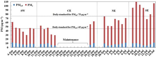
Unlike PM_c, the general levels of PM_2.5 seemed unaffected by the rainy events prior to the sampling campaign, suggesting a predominance of secondary aerosol formation related to the emissions of a local refinery, mobile sources, power plants, and industrial activities; this has been observed previously in the MMA (Mancilla et al. 2015; Martinez et al. 2012). Therefore, it can be inferred that PM_2.5 concentrations in the MMA are strongly influenced by secondary formation processes and, to a lesser extent, primary emissions.

Correlations and ratios (PM and chemical species)

To achieve a better understanding of the PM_c and PM_2.5 concentrations’ behavior, an analysis of their chemical composition was conducted. The chemical characterization of PM_c and PM_2.5 was subject to a regression analysis to determine whether some chemical species originate from different or similar pollutant sources. The overall correlations for PM_c and PM_2.5 are illustrated in Figures 4 and 5, respectively. In addition, the individual correlations for each sampling site are shown in Table 3. Calculated correlation coefficients (r²) were classified into three correlation ranges: good (0.80 < r² < 1.0), moderate (0.50 < r² < 0.80), and weak (r² < 0.50) (Devore 2000). In addition, a p value for each correlation was provided.

Table 3. Individual correlations (R²) for each sampling site.

	OC vs. EC		K vs. K^+		S vs. SO4^2–		Cations vs. anions		Sum 35 metals vs. PM2.5		Cl vs. Cl^–
Site	PM2.5	PMc	PM2.5	PMc	PM2.5	PMc	PM2.5	PMc	PM2.5	PMc	PM2.5	PMc
SW	0.54	0.85	0.66	0.95	0.74	0.61	0.99	0.01	0.11	0.99	*	0.75
CE	0.29	0.64	0.42	0.79	0.85	0.95	0.99	0.52	0.92	0.66	*	0.87
NE	0.00	0.09	0.92	0.83	0.98	0.99	0.95	0.26	0.88	0.95	*	0.99
SE	0.00	0.22	0.74	0.73	0.91	0.99	0.98	0.00	0.52	0.95	*	0.97

Notes. In bold are those correlations that are statistically significant (p value < 0.05) at a confidence level of 95%.

*Correlation was not calculated because Cl and Cl^– concentrations were below the detection limit.

Figure 4. Overall correlations and comparisons between sampling sites for PM_c: (a) OC vs. EC, (b) K vs. K+, (c) S vs. SO₄^2–, (d) cations vs. anions, (e) sum of 35 metals vs. PM_c, and (f) Cl vs. Cl^–. The average errors are OC (16 ± 3%), EC (22 ± 5%), K (19 ± 6%), K⁺ (14 ± 3%), S (20 ± 2%), SO₄^{2 –} (24 ± 3%), cations (> 100%), anions (19 ± 4%), metals (20 ± 5%), and PM_2.5 (8 ± 1%).

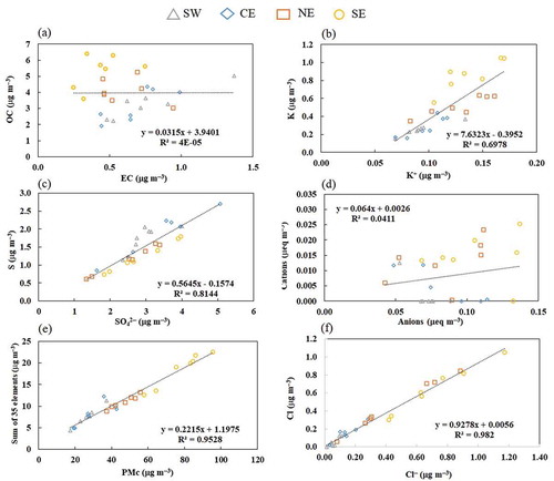
Figure 5. Overall correlations and comparisons between sampling sites for PM_2.5: (a) OC vs. EC, (b) K vs. K⁺, (c) S vs. SO₄^2–, (d) cations vs. anions, (e) sum of 35 metals vs. PM_2.5. The average errors are OC (9.5 ± 0.6%), EC (12 ± 2%), K (43 ± 14%), K⁺ (7.1 ± 0.6%), S (11 ± 0.6%), SO₄^{2 –} (7.1 ± 0.02%), cations (9.5 ± 1.2%), anions (7.4 ± 0.1%), metals (51 ± 12%), and PM_2.5 (7.9 ± 1.2%).

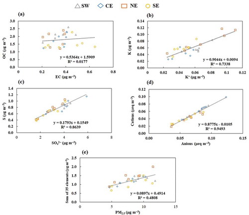
For PM_c, the weak correlations between OC and EC (not significant; p > 0.10) (Figure 4a) demonstrate that there is no direct relationship due to the presence of various emission sources contributing to ambient coarse carbonaceous aerosol in the MMA. It is well known that EC is derived from combustion processes and is emitted mainly as fine particles, whereas OC is organic matter that could have a primary (fine and coarse particles) or secondary origin (mainly fine particles). A good correlation between elemental K and K⁺ (significant; p < 0.001) indicates a contribution from the same sources in each site (Figure 4b). Most K⁺ is emitted from biomass burning (e.g., wood, grass) (Cheng et al. 2013; Chow et al. 2004; Pachon et al. 2013). S and SO₄^{2 –} are well correlated (significant; p < 0.001) at all sites (Figure 4c), suggesting that most of the S measured is in the form of sulfate. The ratios of elemental sulfur (S) to sulfate-sulfur (SS = [SO₄^2–] × 32/96) were calculated and reported in Table 4. A ratio value of unity indicates that most of the S is in the form of sulfate (Shakya and Peltier 2015). The values of the S/SS ratio ranged from 1.2 to 1.8, increasing from east to west, which indicates that there is more sulfur particulate that can be accounted for by inorganic sulfate (White et al. 2005). In addition, this could indicate either sampling/analytical bias or the presence of additional sulfur-containing compounds, given that correlation increases slightly from west to east (Tolocka 2012). The weak correlation between cations and anions (not significant; p > 0.10) (Figure 4d) indicates that there is no neutralization of the aerosol, because the formation of ammonium nitrate might be hindered by sulfate under an ammonia-deficient environment (Tao et al. 2014). The values indicate that anions dominate the ambient air, which is consistent with the dominance of the sulfates. A good correlation between the trace elements and PM_c (significant; p < 0.001) for all sites (Figure 4e) suggests that these metals are predominantly in the PM_c fraction. Finally, a good correlation between Cl and Cl^– (significant; p < 0.001) (Figure 3f) can be associated with sea salts aged during transport from near coastal areas (Yang et al. 2018); these areas are located ~300 km away from the MMA. In addition, other sources associated with Cl emissions include a local refinery in the outskirts and several wastewater treatment plants. This latter is a possible source due to transport from the east and northeast (see Figure 2). Anthropogenic emissions of molecular chlorine photolyze, as well as the resulting Cl, rapidly abstract hydrogen from hydrocarbons, producing HCl that reacts with ammonia to produce ammonium chloride or ammonium nitrate, which can accumulate in particles (Platt 1995; Rossi 2003).

Table 4. Average elemental sulfur (S) to sulfate-sulfur (SS) ratios for each sampling site across the MMA.

	S/SS
	PM2.5		PMc
SW	0.66		1.78
CE	0.65		1.63
NE	0.75		1.37
SE	0.70		1.27

For PM_2.5, weak correlations between EC and OC (not significant; p > 0.10) suggest that they have a different origin (Figure 5a). In the fine fraction, the secondary organic carbon contribution to the total OC tends to be higher. For K⁺, the results indicate common sources (significant; p < 0.001), such as waste incinerators and biomass burning (Cheng et al. 2013) (Figure 5b); typically, combustion processes release fine particles into the air. This confirms the ~0.5% contribution of biomass burning to PM_2.5 observed in the MMA, as estimated by Mancilla et al. (2016) in previous years. Consistent with PM_c, the S measured exhibited the same behavior (significant; p < 0.001), indicating that it is mainly in the form of SO₄^{2 –} (Figure 5c). Here, the S/SS ratios were similar among sampling sites (~0.7), indicating that sulfur is in the form of sulfate (Shakya and Peltier 2015). A good correlation between cations and anions (significant; p < 0.001) indicates that these components are neutralized in the MMA’s PM_2.5 (Figure 5d); this agrees with the results reported by Wang et al. (2013) and Tao et al. (2014). Finally, a weak correlation between trace elements and PM_2.5 (significant; p < 0.001) (Figure 5e) in the SW site indicates that a major fraction of these metals is not emitted in the fine fraction, unlike in PM_c. These elements are tracers for dust resuspension (geological material) that has a particle size in the coarse fraction. The correlation between Cl and Cl^– was not calculated for PM_2.5 because their collected mass in this fraction was below the detection limit and could not be quantified.

Source classification

The average contributions calculated at each sampling site are shown in Figure 6 for PM_c and Figure 7 for PM_2.5. On one hand, the results indicate that the average composition of PM_c is dominated by GM, with a contribution of ~45%. OM is the second largest component, followed by sulfates. Compared to GM, sulfate and OM exhibited higher spatial variability, that is, a higher contribution in the west (sulfates: ~16%; OM: ~17%) than in the east (sulfates: ~5%; OM: ~10%). Here, it is important to observe that unidentified species contribute an average 24% to the composition; this contribution can be comprised of Na, Mg, and missing ions that could not be quantified. On the other hand, the results indicate that the average composition of PM_2.5 is dominated by sulfates, with a higher contribution in the west (~57%) than in the east (~46%). Sulfate is an indicator of the secondary formation of pollutants because of SO₂ oxidation in the atmosphere. In addition, the high contribution of sulfates can be associated with the hygroscopicity behavior of the ammonium sulfate, which increases the particle size at high relative humidity (>70%) (Pilinis and Seinfeld 1987). The second largest component was OM, followed by GM. There was no spatial difference for the OM contribution (~28%), whereas the GM contribution was higher in the east (~13%) than in the west (~8%). The GM contributions were higher in the east, which was probably related to the warmer and dryer conditions that promote dust resuspension; this is consistent with the fact that the final sampling of the campaign was conducted at the east stations, days after the rainy events that occurred prior to the beginning of the sampling campaign. Another important component is EC, which is significantly emitted in the fine fraction; EC is an indicator of the contribution of combustion or burning processes to the observed ambient air concentrations. Finally, it is important to note that all chemical species were blank corrected; for PM_2.5, the most corrected elements were K, Ca, Na, Cr, and Zr, at around 70–90%, while for PM_c, Ca and Na were the major elements corrected, at 20–30%.

Figure 6. Relative contribution (%wt) of the chemical species in the PM_c samples at each site.

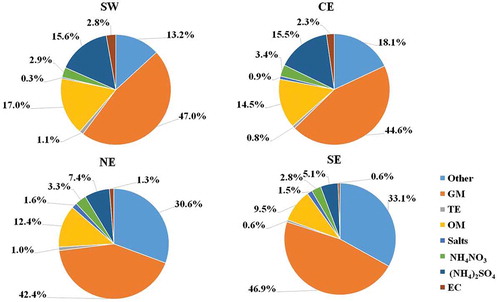
Figure 7. Relative contribution (%wt) of the chemical species in the PM_2.5 samples at each site.

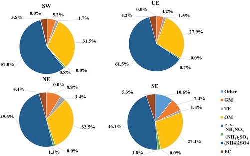
A comparison with other studies conducted in the MMA for different seasons and periods is shown in Table 5. The sulfate content in PM_2.5 was more than twice that obtained for PM_c, because the samples in this study were collected during the summer period; during this period, the PM_2.5 is dominated by acid particles and high secondary aerosol formation (Lee, Wang, and Rusell 2010). The difference for GM may be related to the humidity during the sampling period, which promoted the dust resuspension; there was more humidity during the beginning of the campaign for the SW and CE sites, which exhibited lower contributions of GM, than the humidity recorded at the NE and SE sites. For the coarse particles, GM increased 7%, OM decreased 27%, and sulfates increased twofold compared to the contributions reported by Blanco-Jiménez et al. (2015). The lower contribution of nitrates than reported in previous studies can be attributed to the higher volatilization of nitrates during the summer compared to the winter.

Table 5. Comparison of PM_2.5 and PM_c contributions with those reported by other MMA studies.

	PM2.5			PMc
Reference	Martínez et al. (2012)	Blanco and Mizohata (2015)	This study	Blanco and Mizohata (2015)	This study
Component/Period	November–December 2007	October–December 2014	June–July 2015	October–December 2014	June–July 2015
GM	11	26	6	42	45
TE	1	3	2	3	1
OM*	42	25	30	18	13
Salts	3	2	0	2	1
NH4NO3	13	11	1	8	3
(NH4)2SO4	23	23	54	5	11
EC	7	7	4	2	2
Other	0	2	3	20	24

Notes. *Martínez et al. (2012) used an OM/OC = 1.2; Blanco and Mizohata (2015) used an OM/OC = 1.5; and the present study used an OM/OC = 1.4.

OC and EC concentrations

Average OC and EC concentrations and OC/EC ratios in PM_c and PM_2.5 over the entirety of the sampling campaign are summarized in Table 6. Uncertainties (measurement errors) presented with the average ratios were estimated following uncertainty propagation methods; fractional uncertainties were added in quadrature (Taylor 1997). The OC and EC concentrations in the PM_c fraction were higher than those in the PM_2.5, but in the latter, these species represented a major fraction. OC/EC ratios exceeding 2 can be an indicator of SOA formation (Cao et al. 2004). However, they can also be an indicator of a contribution from other primary sources with a high OC/EC emission ratio (Cabada et al. 2004). The OC/EC ratios for PM_c were higher in the east than in the west, whereas those for PM_2.5 were lower in the east than in the west. A one-way ANOVA was used to determine whether there were any significant differences between average OC/EC ratios of the four sampling sites. For PM_2.5, the ANOVA showed that SW, CE, and NE were spatially similar to one another and spatially different from SE (p < 0.05). A noticeably high OC/EC ratio in the SE suggests a relatively high contribution of SOA. In contrast to the PM_c differences, significant spatial differences were not found across the sampling sites (p > 0.05).

Table 6. Average OC and EC concentrations and OC/EC ratios for PM_c and PM_2.5.

Station	PMc			PM2.5
	OC (μg m^–3)	EC (μg m^–3)	OC/EC	OC (μg m^–3)	EC (μg m^–3)	OC/EC
SW	3.3 ± 0.6	0.77 ± 0.14	4.3 ± 1.1	2.1 ± 0.2	0.36 ± 0.04	5.8 ± 0.9
CE	3.2 ± 0.5	0.68 ± 0.13	4.7 ± 1.2	1.7 ± 0.2	0.35 ± 0.04	4.9 ± 0.9
NE	4.1 ± 0.6	0.61 ± 0.12	6.7 ± 1.7	1.8 ± 0.2	0.32 ± 0.04	5.6 ± 0.9
SE	5.3 ± 0.7	0.44 ± 0.12	12.0 ± 3.6	1.5 ± 0.2	0.42 ± 0.05	3.6 ± 0.5

SOA formation

In this study, the EC-tracer method described in Cabada et al. (2004) was used to estimate the SOA contribution. More information on the method formulation can be found elsewhere (Docherty et al. 2008; Turpin and Huntzicker 1995). The approach of calculating the orthogonal regression using the minimum 20% of the OC/EC ratios was selected to estimate the primary OC/EC; the intercept was discarded for both regressions because of a low contribution from non-combustion sources (e.g., meat cooking operations, biogenic sources) and because a negative intercept has no physical meaning. The primary OC/EC ratio for PM_c was 3.91 ± 0.57, suggesting that most of the primary emissions originate from noncombustion sources, as the ratio is greater than 3 (Cabada et al. 2004; Satsangi et al. 2012). Conversely, the primary OC/EC ratio for PM_2.5 was 1.0 ± 0.8, suggesting that primary emissions originate from fossil fuel combustion sources, as the OC/EC ratio is low (Cabada et al. 2004; Satsangi et al. 2012).

As can be seen in Table 7, SOA contribution was constant and very low for PM_c; in contrast, for PM_2.5, it increased from east to west as a result of the chemical processing of the fresh emissions, rich in SOA precursors, which produced more SOA as the air masses aged over the course of their movement toward the west. A higher contribution of SOA to the total organic aerosol was probably due to atmospheric oxidation during transport and the relatively small contribution from local primary emission sources. For PM_c, the relatively low contribution of SOA is clearly associated with noncombustion sources such as dust resuspension, as discussed in the following. For PM_2.5, the SOA contribution to the organic aerosol was higher than 70% for all sampling sites; these results are similar to those estimated by Mancilla et al. (2015) in the MMA and are consistent with those reported for other urban areas (Hayes et al. 2013; Peng et al. 2016, Zhang et al. 2011). A one-way ANOVA was used to test for spatial differences in SOA formation using the SOA concentrations. Spatial differences for PM_c and PM_2.5 were found across the sampling sites (p < 0.05). For both cases, the remarkable finding is that SW and SE were quite different. In order to estimate the SOA a value of 1.4 for the OM/OC ratio was used.

Table 7. Average SOA contributions for PM_c and PM_2.5 in the MMA.

Site	(SOA)PMc (μg m^–3)	(SOA/OA)PMc	SOA/PMc	(SOA)PM2.5 (μg m^–3)	(SOA/OA)PM2.5	SOA/PM2.5
SW	1.4 ± 1.6	0.2 ± 0.1	0.04 ± 0.03	2.5 ± 0.7	0.8 ± 0.2	0.3 ± 0.1
CE	1.2 ± 1.5	0.2 ± 0.1	0.03 ± 0.03	1.9 ± 0.6	0.8 ± 0.3	0.3 ± 0.1
NE	4.0 ± 1.4	0.5 ± 0.2	0.04 ± 0.03	2.1 ± 0.6	0.8 ± 0.3	0.3 ± 0.1
SE	5.3 ± 1.2	0.6 ± 0.2	0.04 ± 0.01	1.5 ± 0.7	0.7 ± 0.3	0.2 ± 0.1

Enrichment factors

The average EF values for PM_c and PM_2.5 are shown in Figures 8 and 9, respectively. On one hand, it can be observed that most of the trace elements enrich from east to west. This trend suggests that those elements are continuously emitted over the MMA and that they accumulate because of the transport effect. As noted in the preceding, the air masses during the campaign moved from the northeast to the west, promoting the transport of pollutants in that direction. On the other hand, some elements—that is, Ti, Cl, K, Rb, Cd, Y, and Fe—enrich in the opposite direction, suggesting that those elements are emitted by a point source located in the east, for example, the cement and steel companies, two of the major industries in the MMA.

Figure 8. Enrichment factor value for PM_c using the concentration of the trace elements in the four sampling sites in the MMA, taking Ca as reference element.

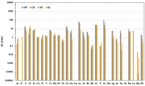
Figure 9. Enrichment factor value for PM_2.5 using the concentration of the trace elements in the four sampling sites in the MMA, taking Ca as reference element.

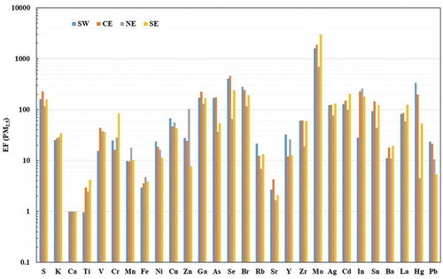
For PM_c, it was seen that Ni, Rb, Y, In, Hg, Sb, and Ga exhibited EFs < 1, suggesting that these are depleted while air masses move through the urban area and are crustal in origin. The high EF values for S, Cl, Zr, La, As, Cr, K, Sr, Ba, and Cu indicate that these elements originate mainly from anthropogenic sources. It should be noted that EF values for S, Cl, and K are consistent with the high correlations discussed previously. The EF values for K and Cl support the hypothesis that they originate from biomass burning in the former case and industrial activities in the latter and that their sources are located mainly in the east. For S, the EF values suggest a contribution by inorganic sulfate. The EF of S increases from east to west because of S that may come from the refinery and fresh emissions that occur in the west. Ba, which is enriched to the west, has a stronger association with unleaded fuel and diesel oil-powered vehicles (Monaci et al. 2000). This is expected, given the abundance of freight transport associated to industrial activity. Arsenic is a toxic and carcinogenic element, and it is released into the atmosphere from the smelting of metals, combustion of fuels, and use of pesticides (Sánchez-Rodas et al. 2007); the EF values increase toward the west. Cu is associated with industry and road traffic; it increases from east to west. Based on the low EF values for Pb, it can be assumed that the dust in the MMA contains this element as a result of the many decades of leaded gasoline use and the use of Pb in other industries’ manufacturing and chemical processes (Smichowski et al. 2008; Valdez Cerda et al. 2011); however, its increase from east to west is due to dust resuspension and transport phenomena.

For PM_2.5, a major enrichment in transition metals was found. The EF values for these elements increase from east to west. These higher EF values are associated with industrial areas (Schaumann et al. 2004). Higher EF values were found for La, indicating the presence of catalytic cracking processes, whereas V and Ni suggest fossil fuel combustion sources such as vehicles, cooking operations, petroleum coke, and power plants (Kulkarni, Chellam, and Fraser 2006). Here, the crustal elements are associated with the construction industry (Wu et al. 2007), unlike for PM_c, for which they are associated with street dust resuspension. Hg combined with Pb and K is a good indicator of waste incinerators, whereas a combination with As is associated with coal combustion (Kolker et al. 2013). This can be associated with the open biomass burning and charcoal combustion in the east of the MMA. In addition, the presence of S is a good indicator of vehicular (particularly diesel) and refinery emissions; Pb can also originate from brake and tire wear (Morawska and Zhang 2002). The high EF values for Br, Cu, and Mo for both PM_c and PM_2.5 suggest an important contribution of traffic emissions (Smichowski et al. 2008; Zereini et al. 2005).

Conclusion

This study provides evidence of the spatial behavior of PM_2.5 and PM_c in the Monterrey Metropolitan area. It illustrates some spatial differences among sampling sites for PM_c, showing an increment trend from east to west, whereas it showed more homogeneous spatial concentrations for PM_2.5. In addition, this was consistent with the enrichment of trace elements from east to west. PM_c is the major fraction of PM₁₀, which comprises more than 75%. The PM_2.5 levels were typically associated with high contributions of SO₄^2–, OM, and EC, which are commonly associated with anthropogenic sources, whereas the high PM_c levels were related mainly to geological material, which is commonly associated with dust resuspension. Based on the OC/EC values, the results indicate that SOA accounted for 70% of the observed organic aerosol in PM_2.5. Finally, EFs indicate that most of the trace elements have a crustal origin for PM_c and an anthropogenic origin for PM_2.5.

Acknowledgment

The authors greatly appreciate the support of the MMA’s Integrated Environmental Monitoring System (or SIMA, to use the initials of its Spanish name).

Disclosure statement

No potential conflict of interest was reported by the authors.

Additional information

Funding

This study was supported by the Secretariat of the Sustainable Development of the government of the state of Nuevo León (grant no. IA-919002997-N186-2014 (74/14)).

Notes on contributors

Y. Mancilla

Y. Mancilla is a researcher at the School of Engineering and Science, Tecnologico de Monterrey, in Monterrey, Mexico.

I.Y. Hernandez Paniagua

I.Y. Hernandez Paniagua is a scientist at the Centro de Ciencias de la Atmósfera, Universidad Nacional Autónoma de Mexico, in Mexico.

A. Mendoza

A. Mendoza is a research professor at the School of Engineering and Science, Tecnologico de Monterrey, in Monterrey, Mexico.

References

- Atkinson, R. W., G. W. Fuller, H. R. Anderson, R. M. Harrison, and B. Armstrong. 2010. Urban ambient particle metrics and health: A time-series analysis. Epidemiology 21:501–11. doi:10.1097/EDE.0b013e3181e9edc4.
- Badillo-Castañeda, C. T., L. Garza-Ocañas, M. C. H. Garza-Ulloa, M. T. Zanatta-Calderón, and A. Caballero-Quintero. 2015. Heavy metal content in PM2.5 air samples collected in the Metropolitan Area of Monterrey, México. Hum. Ecol. Risk Assess. 21:2022–35. doi:10.1080/10807039.2015.1017873.
- Birch, M. E., and R. A. Cary. 1996. Elemental carbon-based method for monitoring occupational exposures to particulate diesel exhaust: Methodology and exposure issues. Analyst 121:1183–90. doi:10.1039/an9962101183.
- Blanco-Jiménez, S., F. Altúzar, B. Jiménez, G. Aguilar, M. Pablo, and M. A. Benítez. 2015. Evaluación de partículas suspendidas PM2.5 en el Área Metropolitana de Monterrey, 34. México: Instituto Nacional de Ecología y Cambio Climático (INECC).
- Cabada, J. C., N. P. Spyros, R. Subramanian, A. L. Robinson, A. Polidori, and B. Turpin. 2004. Estimating the secondary organic aerosol contribution to PM2.5 using the EC tracer method. Aerosol. Sci. Technol. 38:140–55. doi:10.1080/02786820390229084.
- Cambra-Lopez, M., A. J. A. Aarnink, Y. Zhao, S. Calvet, and A. G. Torres. 2010. Airborne particulate matter from livestock production systems: A review of an air pollution problem. Environ. Pollut. 158:1–17. doi:10.1016/j.envpol.2010.05.018.
- Chatterjee, M., E. V. Silva Filho, S. K. Sarkar, S. M. Sella, A. Bhattacharya, K. K. Satpathy, M. V. Prasad, S. Chakraborty, and B. D. Bhattacharya. 2007. Distribution and possible source of trace elements in the sediment cores of a tropical macrotidal estuary and their ecotoxicological significance. Environ. Int. 33:346–56. doi:10.1016/j.envint.2006.11.013.
- Chen, R., Y. Li, Y. Ma, G. Pan, G. Zeng, X. Xu, B. Chen, and H. Kan. 2011. Coarse particles and mortality in three Chinese cities: The China Air Pollution and Health Effects Study (CAPES). Sci. Total Environ. 409:4934–38. doi:10.1016/j.scitotenv.2011.08.058.
- Cheng, Y., G. Engling, K.-B. He, F.-K. Duan, Y.-L. Ma, Z.-Y. Du, J.-M. Liu, M. Zheng, and R. J. Weber. 2013. Biomass burning contribution to Beijing aerosol. Atmos. Chem. Phys. 13:7765–81. doi:10.5194/acp-13-7765-2013.
- Chow, J. C., J. G. Watson, H. Kuhns, V. Etyemezian, D. H. Lowenthal, D. Crow, S. D. Kohl, J. P. Engelbrecht, and M. C. Green. 2004. Source profiles for industrial, mobile, and area sources in the Big Bend Regional Aerosol Visibility and Observational study. Chemosphere 54:185–208. doi:10.1016/j.chemosphere.2003.07.004.
- Clements, A. L., M. P. Fraser, N. Upadhyay, P. Herckes, M. Sundblom, J. Lantz, and P. A. Solomon. 2013. Characterization of summertime coarse particulate matter in the Desert Southwest-Arizona, USA. J. Air Waste Manage. Assoc. 63:764–72. doi:10.1080/10962247.2013.787955.
- Davidson, C. I., R. F. Phalen, and P. A. Solomon. 2005. Airborne particulate matter and human health: A review. Aerosol. Sci. Tech. 39:737–49. doi:10.1080/02786820500191348.
- Docherty, K. S., E. A. Stone, I. M. Ulbrich, P. F. DeCarlo, D. C. Snyder, J. J. Schauer, R. E. Peltier, R. J. Weber, S. M. Murphy, J. H. Seinfeld, et al. 2008. Apportionment of primary and secondary organic aerosols in southern California during the 2005 study of organic aerosols in riverside (SOAR-1). Environ. Sci. Technol. 42:7655–62. doi:10.1021/es8008166.
- El-Zanan, H. S., B. Zielinska, L. R. Mazzoleni, and D. Hansen. 2009. Analytical determination of the aerosol organic mass-to-organic carbon ratio. J. Air Waste Manage. Assoc. 59:58–69. doi:10.3155/1047-3289.59.1.58.
- Enamorado-Báez, S. M., J. M. Gómez-Guzmán, E. Chamizo, and J. M. Abril. 2015. Levels of 25 trace elements in high-volume air filter samples from Seville (2001-2002): Sources, enrichment factors and temporal variations. Atmos. Res. 155:118–29. doi:10.1016/j.atmosres.2014.12.005.
- Garza-Ocañas, L., H. Garza-Ulloa, O. González-Santiago, R. Lujan-Rangel, and C. T. Badillo-Castañeda. 2010. PM2.5-bounded PAHs from two zones of the Metropolitan Area of Monterrey, Nuevo Leon, Mexico. Toxicol. Lett. 196:S287. doi:10.1016/j.toxlet.2010.03.906.
- George, I. J., and J. P. D. Abbatt. 2010. Heterogeneous oxidation of atmospheric aerosol particles by gas-phase radicals. Nat. Chem. 2:713722. doi:10.1038/Nchem.806.
- González Cárdenas, J. A. 2014. Determinación y cuantificación de PAHs en partículas PM2.5 en el Área Metropolitana de Monterrey y su relación con el 1-hidroxipireno como marcador biológico de exposición. Doctorade Thesis, UANL, Faculty of Medicine.
- González, L. T., F. E. L. Rodríguez, M. Sánchez-Domínguez, C. Leyva-Porras, L. G. Silva-Vidaurri, K. Acuna-Askar, B. I. Kharisov, J. F. Villarreal Chiu, and J. M. Alfaro Barbosa. 2016. Chemical and morphological characterization of TSP and PM2.5 by SEM-EDS, XPS and XRD collected in the metropolitan area of Monterrey, Mexico. Atmos. Environ. 143:249–60. doi:10.1016/j.atmosenv.2016.08.053.
- González-Santiago, O., C. T. Badillo-Castañeda, J. D. W. Kahl, E. Ramírez-Lara, and I. Balderas-Rentería. 2011. Temporal analysis of PM10 in Metropolitan Monterrey, México. J. Air Waste Manage. Assoc. 61:573–79. doi:10.3155/1047-3289.61.5.573.
- Graff, D. W., W. E. Cascio, A. Rappold, H. Zhou, Y.-C. T. Huang, and R. B. Devlin. 2009. Exposure to concentrated coarse air pollution particles causes mild cardiopulmonary effects in healthy young adults. Environ. Health Persp. 117:1089–94. doi:10.1289/ehp.0900558.
- Grahame, T. J., R. Klemm, and R. B. Schlesinger. 2014. Public health and components of particulate matter: The changing assessment of black carbon. J. Air Waste Manage. Assoc. 64:620–60. doi:10.1080/10962247.2014.912692.
- Hayes, P. L., A. M. Ortega, M. J. Cubison, K. D. Froyd, Y. Zhao, S. S. Cliff, W. W. Hu, D. W. Toohey, J. H. Flynn, B. L. Lefer, et al. 2013. Organic aerosol composition and sources in Pasadena, California during the 2010 CalNex campaign. J. Geophys. Res. 118:9233–57.
- Hernández Paniagua, I. Y., K. C. Clemitshaw, and A. Mendoza. 2017. Observed trends in ground-level O3 in Monterrey, Mexico during 1993-2014: Comparison with Mexico City and Guadalajara. Atmos. Chem. Phys. 17:9163–85. doi:10.5194/acp-17-9163-2017.
- Hinojosa-Velasco, A., V. J. Lara-Díaz, G. M. Mejía-Velázquez, and J. Santos-Guzmán. 2010. Air pollution effects (PM10 and PM2.5) in neonatal mortality in a metropolitan area in the northeast of México. 15th International Union of Air Pollution Prevention and Enviromental Protection Association (IUAPPA), Canada, September.
- Ito, K., R. Mathes, Z. Ross, A. Nádas, G. Thurston, and T. Matte. 2011. Fine particulate matter constituents associated with cardiovascular hospitalizations and mortality in New York City. Environ. Health Persp. 119:467–73. doi:10.1289/ehp.1002667.
- Jimenez, J. L., M. R. Canagaratna, N. M. Donahue, A. S. H. Prevot, Q. Zhang, J. H. Kroll, P. F. DeCarlo, J. D. Allan, H. Coe, N. L. Ng, et al. 2009. Evolution of organic aerosols in the atmosphere. Science 326:1525–29. doi:10.1126/science.1180353.
- Kolker, A., M. A. Engle, B. Peucker-Ehrenbrink, N. J. Geboy, D. P. Krabbenhoft, M. H. Bothner, and M. T. Tate. 2013. Atmospheric mercury and fine particulate matter in coastal New England: Implications for mercury and trace element sources in the northeastern United States. Atmos. Environ. 79:760–68. doi:10.1016/j.atmosenv.2013.07.031.
- Kulkarni, P., S. Chellam, and M. P. Fraser. 2006. Lanthanum and lanthanides in atmospheric fine particles and their apportionment to refinery and petrochemical operations in Houston, TX. Atmos. Environ. 40:508–20. doi:10.1016/j.atmosenv.2005.09.063.
- Ledoux, F., A. Kfoury, G. Delmaire, G. Roussel, A. El Zein, and D. Courcot. 2017. Contributions of local and regional anthropogenic sources of metals in PM2.5 at an urban site in northern France. Chemosphere 181:713–24. doi:10.1016/j.chemosphere.2017.04.128.
- Lee, B. K., and N. T. Hieu. 2011. Seasonal variation and source of heavy elements in atmospheric aerosols in a residential area of Ulsan, Korea. Aerosol. Air Qual. Res. 11:679–88. doi:10.4209/aaqr.2010.10.0089.
- Lee, S., Y. Wang, and A. Rusell. 2010. Assessment of secondary organic carbon in the southeastern United States: A review. J. Air Waste Manage. Assoc. 60 (11):1282–92. doi:10.3155/1047-3289.60.11.1282.
- Lippmann, M. 2011. Particulate matter (PM) air pollution and health: Regulatory and policy implications. Air Qual. Atmos. Health 5:237–41. doi:10.1007/s11869-011-0136-5.
- López, J. M., M. S. Callén, R. Murillo, T. García, M. V. Navarro, M. T. de la Cruz, and A. M. Mastral. 2005. Levels of selected metals in ambient air PM10 in an urban site of Zaragoza (Spain). Environ. Res. 99:58–67. doi:10.1016/j.envres.2005.01.007.
- Loska, K., D. Wiechula, and I. Korus. 2004. Metal contamination of farming soils affected by industry. Environ. Int. 30:159–65. doi:10.1016/S0160-4120(03)00157-0.
- Mallone, S., M. Stafoggia, A. Faustini, G. P. Gobbi, A. Marconi, and F. Forastiere. 2011. Saharan dust and associations between particulate matter and daily mortality in Rome, Italy. Environ. Health Perspect 119:1409–14. doi:10.1289/ehp.119-a484.
- Mancilla, Y., A. E. Araizaga, and A. Mendoza. 2012. A tunnel study to estimate emission factors from mobile sources in Monterrey, Mexico. J. Air Waste Manage. Assoc. 62:1431–42. doi:10.1080/10962247.2012.717902.
- Mancilla, Y., P. Herckes, M. P. Fraser, and A. Mendoza. 2015. Secondary organic aerosol contributions to PM2.5 in Monterrey, Mexico: Temporal and seasonal variation. Atmos. Res. 153:348–59. doi:10.1016/j.atmosres.2014.09.009.
- Mancilla, Y., and A. Mendoza. 2012. A Tunnel Study to Characterize PM2.5 Emissions from Gasoline-Powered Vehicles in Monterrey, Mexico. Atmos. Environ. 59:449–60. doi:10.1016/j.atmosenv.2012.05.025.
- Mancilla, Y., A. Mendoza, M. P. Fraser, and P. Herckes. 2016. Organic composition and source apportionment of fine aerosol at Monterrey, Mexico, based on organic markers. Atmos. Chem. Phys. 16:953–70. doi:10.5194/acp-16-953-2016.
- Martínez, M. A., P. Caballero, O. Carrillo, A. Mendoza, and G. M. Mejía. 2012. Chemical characterization and factor analysis of PM2.5 in two sites of Monterrey, Mexico. J. Air Waste Mange. Assoc. 62:817–27. doi:10.1080/10962247.2012.681421.
- Medina Gaitán, G. E. 2015. Desarrollo de perfiles de emisión de la fracción orgánica del PM2.5 en el Área Metropolitana de Monterrey. Master Thesis, Tecnologico de Monterrey, December.
- Meister, K., C. Johansson, and B. Forsberg. 2012. Estimated short-term effects of coarse particleson daily mortality in Stockholm, Sweden. Environ. Health Perspect. 120:431–36. doi:10.1289/ehp.1103995.
- Mejía-Velázquez, G. M., and C. Lerma-Serna. 2013. Evaluation of increased health risks associated to PM10 pollution in the monterrey metropolitan area. 106th A&WMA Annual Conference and Exhibition, USA, June.
- Minguillón, M. C., X. Querol, U. Baltensperger, and A. S. H. Prévot. 2012. Fine and coarse PM composition and sources in rural and urban sites in Switzerland: Local or regional pollution? Sci. Total Environ. 427-428:191–202. doi:10.1016/j.scitotenv.2012.04.030.
- Monaci, F., F. Moni, E. Lanciotti, D. Grechi, and R. Bargagli. 2000. Biomonitoring of airborne metals in urban environments: New tracers of vehicle emissions, in place of lead. Environ. Pollut. 107:321–27. doi:10.1016/S0269-7491(99)00175-X.
- Morawska, L., and J. Zhang. 2002. Combustion sources of particles. 1. Health relevance and source signatures. Chemosphere 49:1045–58. doi:10.1016/S0045-6535(02)00241-2.
- NIOSH. 2003. Manual of analytical methods (NMAM). In Monitoring of diesel particulate exhaust in the workplace, Chapter Q, third supplement to NMAM, ed. P. F. O’Connor and P. C. Schlecht, 4th ed., 1-154. Cincinnati, OH: NIOSH. DHHS (NIOSH) Publication No. 2003-154.
- Ostro, S. D., W.-Y. Feng, R. Broadwin, B. J. Malig, R. S. Green, and M. J. Lipsett. 2008. The impact of components of fine particulate matter on cardiovascular mortality in susceptible subpopulations. Occup. Environ. Med. 11:750–56. doi:10.1136/oem.2007.036673.
- Pachon, J. E., R. J. Weber, X. Zhang, J. A. Mulholland, and A. G. Russell. 2013. Revising the use of potassium (K) in the source apportionment pf PM2.5. Atmos. Pollut. Res. 4:14–21. doi:10.5094/APR.2013.002.
- Peng, J., M. Hu, Z. Gong, X. Tian, M. Wang, J. Zheng, Q. Guo, W. Cao, W. Lv, W. Hu, et al. 2016. Evolution of secondary inorganic and organic aerosol during transport: A case study at a regional receptor site. Environ. Pollut. 218:794–803. doi:10.1016/j.envpol.2016.08.003.
- Pilinis, C., and J. H. Seinfeld. 1987. Continued development of a general equilibrium model for inorganic multicomponent atmospheric aerosols. Atmos. Environ. 21:2453–66. doi:10.1016/0004-6981(87)90380-5.
- Pinto, J. P., A. S. Lefohn, and D. S. Shadwick. 2004. Spatial variability of PM2.5 in urban areas in the United States. J. Air Waste Mange. Assoc. 54:440–49. doi:10.1080/10473289.2004.10470919.
- Platt, U. 1995. The chemistry of halogen compounds in the Arctic troposphere, in Tropospheric Oxidation Mechanisms, K. H. Becker, ed., European Commission. Report EUR 16171 EN, Luxembourg, 9–20.
- Pope, C. A., III, R. D. Brook, R. T. Burnett, and D. W. Dockery. 2011. How is cardiovascular disease mortality risk affected by duration and intensity of fine particulate matter exposure? An integration of the epidemiologic evidence. Air Qual. Atmos. Health 4:5–14. doi:10.1007/s11869-010-0082-7.
- Reimann, C., and P. Caritat. 2005. Distinguishing between natural and anthropogenic sources for elements in the environment: Regional geochemical surveys versus enrichment factors. Sci. Total Environ. 337:91–107. doi:10.1016/j.scitotenv.2004.06.011.
- Richard, A., M. F. D. Gianini, C. Mohr, M. Furger, N. Bukowiecki, M. C. Minguillon, P. Lienemann, U. Flechsig, K. Appel, P. F. DeCarlo, et al. 2011. Source apportionment of size and time resolved trace elements and organic aerosols from an urban courtyard site in Switzerland. Atmos. Chem. Phys. 11:8945–63.
- Rojas-Moreno, A., J. Santos-Guzmán, B. H. Lapizco-Encinas, and G. M. Mejía-Velázquez. 2008. Evaluation of visits to hospitals with PM10 and PM2.5 concentration levels in the MMA. 101 AWMA Conference, USA, June.
- Rossi, M. J. 2003. Heterogeneous reactions on salts. Chem. Rev. 103:4823–82. doi:10.1021/cr020507n.
- Ruthenburg, T. C., P. C. Perlin, V. Liu, C. E. McDade, and A. M. Dillner. 2014. Determination of organic matter and organic matter to organic carbon ratios by infrared spectroscopy with application to selected sites in the IMPROVE network. Atmos. Environ. 86:47–57. doi:10.1016/j.atmosenv.2013.12.034.
- Sánchez-Rodas, D., A. M. Sánches de la Campa, J. D. de la Rosa, V. Oliveira, J. L. Gómez-Ariza, X. Querol, and A. Alastuey. 2007. Arsenic speciation of atmospheric particulate matter (PM10) in an industrialised urban site in southwestern Spain. Chemosphere 66:1485–93. doi:10.1016/j.chemosphere.2006.08.043.
- Satsangi, A., T. Pachauri, V. Singla, A. Lakhani, and K. M. Kumari. 2012. Organic and elemental carbon aerosols at a suburban site. Atmos. Res. 113:13–21. doi:10.1016/j.atmosres.2012.04.012.
- Schaumann, F., P. J. A. Borm, A. Herbrich, J. Knoch, M. Pitz, R. P. F. Schins, B. Luettig, J. M. Hohlfeld, J. Heinrich, and N. Krug. 2004. Metal-rich ambient particles (Particulate Matter 2.5) cause airway inflammation in healthy subjects. Am. J. Respir. Critical Care Med. 170:898–903. doi:10.1164/rccm.200403-423OC.
- Seinfeld, J. H., and S. N. Pandis. 2006. Atmospheric chemistry and physics: From air pollution to climate change. New York: J. Wiley.
- Shakya, K. M., and R. E. Peltier. 2015. Non-sulfate sulfur in fine aerosols across the United States: Insight for organosulfate prevalence. Atmos. Environ. 100:159–66. doi:10.1016/j.atmosenv.2014.10.058.
- Shelley, R. U., P. L. Morton, and W. M. Landing. 2015. Elemental ratios and enrichment factors in aerosols from the US-GEOTRACES North Atlantic transects. Deep-Sea Res. II 116:262–72. doi:10.1016/j.dsr2.2014.12.005.
- Shridhar, V., P. S. Khillare, T. Agarwal, and S. Ray. 2010. Metallic species in ambient particulate matter at rural and urban location of Delhi. J. Hazard Mater 175:600–07. doi:10.1016/j.jhazmat.2009.10.047.
- Smichowski, P., D. Gómez, C. Frazzoli, and S. Caroli. 2008. Traffic-related elements in airborne particulate matter. Appl. Spectrosc. Rev. 43:23–49. doi:10.1080/05704920701645886.
- Sprovieri, F., M. Bencardino, F. Cofone, and N. Pirrone. 2011. Chemical composition of aerosol size fractions at a coastal site in Southwestern Italy: Seasonal variability and transport influence. J. Air Waste Manage. Assoc. 61:941–51. doi:10.1080/10473289.2011.599267.
- Sprovieri, F., and N. Pirrone. 2008. Particle size distributions and elemental composition of atmospheric particulate matter in southern Italy. J. Air Waste Manage. Assoc. 58:797–805. doi:10.3155/1047–3289.58.6.797.
- Tao, Y., Z. Yin, Z. Ye, Z. Ma, and J. Chen. 2014. Size distribution of water-soluble inorganic aerosols in Shanghai. Atmos. Pollut. Res. 5:639–47. doi:10.5094/APR.2014.073.
- Taylor, J. R. 1997. Error analysis: The study of uncertainties in physical measurements. Mill Valley, California: University Science Books.
- Tobías, A., L. Pérez, J. Díaz, C. Linares, J. Pey, A. Alastruey, and X. Querol. 2011. Short-term effects of particulate matter on total mortality during Saharan dust outbreaks: A case-crossover analysis in Madrid (Spain). Sci. Total Environ. 412–413:386–89. doi:10.1016/j.scitotenv.2011.10.027.
- Tolocka, M. P. 2012. Contribution of organosulfur compounds to organic aerosol mass. Environ. Sci. Technol. 46:7978–83. doi:10.1021/es300651v.
- Trifuoggi, M., C. Donadio, O. Mangoni, L. Ferrara, F. Bolinesi, R. A. Nastro, C. Stanislao, M. Toscanesi, G. Di Natale, and M. Arienzo. 2017. Distribution and enrichment of trace metals in Surface marine sediments in the Gulf of Pozzuoli and off the coast of the brownfield metallurgical site of Ilva of Bagnoli (Campania, Italy). Mar. Pollut. Bull. 124:502–11. doi:10.1016/j.marpolbul.2017.07.033.
- Turpin, B. J., and J. J. Huntzicker. 1995. Identification of secondary organic aerosol episodes and quantitation of primary and secondary organic aerosol concentrations during SCAQS. Atmos. Environ. 29:3527–44. doi:10.1016/1352-2310(94)00276-q.
- Turpin, B. J., and H.-J. Lim. 2001. Species contributions to PM2.5 mass concentrations: Revisiting common assumptions for estimating organic mass. Aerosol. Sci. Tech. 35:602–10. doi:10.1080/02786820119445.
- Valdez Cerda, E., L. Hinojosa Reyes, J. M. Alfaro Barbosa, P. Elizondo-Martínez, and K. Acuña-Askar. 2011. Contamination and chemical fractionation of heavy metals in street dust from the Metropolitan Area of Monterrey, Mexico. Environ. Technol. 32:1163–72. doi:10.1080/09593330.2010.529466.
- Vega, E., E. Reyes, H. Ruiz, J. Garcia, G. Sanchez, G. Martinez, and U. Gonzalez. 2004. Analysis of PM2.5 and PM10 in the atmosphere of Mexico City during 2000–2002. J. Air Waste Manag. Assoc. 54:786–98. doi:10.1080/10473289.2004.10470952.
- Wang, L., H. H. Du, J. M. Chen, M. Zhang, X. Y. Huang, H. B. Tan, L. D. Kong, and F. H. Geng. 2013. Consecutive transport of anthropogenic air masses and dust storm plume: Two case events at Shanghai, China. Atmos. Res. 127:22–33. doi:10.1016/j.atmosres.2013.02.011.
- World Health Organization, Switzerland. 2006. WHO air quality guidelines for particulate matter, ozone, nitrogen, dioxide and sulfur dioxide. Accessed September 2018. http://apps.who.int/iris/bitstream/handle/10665/69477/WHO_SDE_PHE_OEH_06.02_eng.pdf;jsessionid=F5D474862A226F880893E3B34A546114?sequence=1.
- Wu, Y. S., G. C. Fang, W. J. Lee, J. F. Lee, C. C. Chang, and C. Z. Lee. 2007. A review of atmospheric fine particulate matter and its associated trace metal pollutants in Asian countries during the period 1995–2005. J. Hazard Mater 143:511–15. doi:10.1016/j.jhazmat.2006.09.066.
- Yang, X., T. Wang, M. Xia, X. Gao, Q. Li, N. Zhang, Y. Gao, S. Lee, X. Wang, L. Xue, et al. 2018. Abundance and origin of fine particulate chloride in continental China. Sci. Total Environ. 624:1041–51. doi:10.1016/j.scitotenv.2017.12.205.
- Yaroshevsky, A. 2006. Abundances of chemical elements in the Earth’s crust. Geochem. Int. 44:48–55. doi:10.1134/S001670290601006X.
- Zereini, F., F. Alt, J. Messerschmidt, C. Wiseman, I. Feldmann, A. V. Bohlen, J. Müller, K. Liebl, and W. Püttmann. 2005. Concentration and distribution of heavy metals in urban airborne particulate matter in Frankfurt am Main, Germany. Environ. Sci. Technol. 39:2983–89.
- Zhang, F., J. Zhao, J. Chen, Y. Xu, and L. Xu. 2011. Pollution characteristics of organic and elemental carbon in PM2.5 in Xiamen, China. J. Environ. Sci. 23:1342–49. doi:10.1016/S1001-0742(10)60559-1.
- Zhang, R. Y., A. Khalizov, L. Wang, M. Hu, and W. Xu. 2012. Nucleation and growth of nanoparticles in the atmosphere. Chem. Rev. 112:1957–2011. doi:10.1021/Cr2001756.