Detection of anomalous nitrogen dioxide (NO₂) concentration in urban air of India using proximity and clustering methods

ABSTRACT

Owing to accurate future air quality estimates, need for detecting the anomalously high increase in concentration of pollutants cannot be adjourned. Plentiful approaches were proposed in the past to substantially determine the abnormal conditions, but most of the statistical approaches were computationally expensive and ignored the false alarm ratios. Thus, a hybrid of proximity- and clustering-based anomaly detection approaches to identify anomalies in the air quality data is suggested in this work. The Gaussian distribution property of the real-world data set is utilized further to segregate out anomalies. The results depicted twofold advantages of our approach, by efficient extraction of anomalies and with increased accuracy by reducing the number of false alarms. Specifically, the presence of NO₂ concentration in air is investigated in this work, considering its constant increase over decades as well as its inevitable health risks. Furthermore, spatiotemporal segments with anomalously high NO₂ concentrations for 14 residential, industrial, and commercial areas of five cities in India are extracted. To validate the results, a comparative analysis with existing approaches of anomaly detection and with two benchmark data sets is performed. Results showed that our method outperformed the existing methods of anomaly detection, when evaluated over metrics such as sensitivity, miss rate, and false alarms. Further, a detailed analysis of extracted anomalies and a detailed discussion about the factors responsible for such anomalies are presented in this work. This study is helpful in educating government and people about spatiotemporal, geographical, and economic conditions responsible for anomalously high NO₂ concentrations in air.

Implications: Using our methodology, days with extremely high concentration of any pollutant in air, at any particular location, can be extracted. The reasons for such extremely high pollutant concentration on particular days of a year can be studied and preventive measures can be taken by the government. Thus, by identification of causes of anomalies, future similar events can be avoided. This would also help in people’s decision making in case such events occur in the future.

Introduction

Among several definitions of a smart city (Ramaprasad, Sánchez-Ortiz, and Syn 2017), one defines this as an urban settlement that utilizes the data generated in order to solve issues such as traffic, waste, mobility, and so on. One of these issues is air pollution. Despite the govenment’s implementation of policies, air quality in India is degrading day by day (Dholakia et al. 2013). As a consequence, an urgent need to find an adequate solution to air-quality-related issues cannot be ignored. Air pollution comprises the presence of exceeding amounts of certain pollutants in the atmosphere. Pollutants provoking severe health drawbacks include nitrogen dioxide, nitric oxide, sulfur dioxide, carbon monoxide, particulate matter, and so on (Pandey, Kumar, and Devotta 2005). Specifically, in this work nitrogen dioxide (NO₂) is focused upon, and is among the primary pollutants found in the air (Kumar and Joseph 2006) of urban cities of India. NO₂ is highly hazardous for the environment (Agrawal et al. 2003) and for human health (Latza, Gerdes, and Baur 2009), causing severe health problems in humans, such as reduction in visibility and respiratory issues (Pandey, Kumar, and Devotta 2005). Study of NO₂ is important because it is toxic and participates in catalytic cycles producing other secondary pollutants such as ozone and acid rain. Availability of data and constantly increasing presence of NO₂ concentration each year, in the air of urban areas of India, was the primary reason for selection of NO₂ in the proposed work.

Air quality data used in this work consisted of measurements taken from air quality stations installed by the Central Pollution Control Board, Delhi. This data might contain uncertainties due to equipment malfunction or terrain related issues (Araki et al. 2017). However, even after not considering such noisy measurements, there were still anomalies in the data due to abnormal behavior of pollutants caused by various other factors, showing a sudden steep increase (or decrease) in the pollution levels. Essentially, anomalies are the data points that differ significantly from rest of the data points (Han, Pei, and Kamber 2011). For our work, anomalies were the days with extremely high concentrations of NO₂ with respect to all other days of a month. It was quite important to extract such anomalies that might affect the government’s and people’s decision making in planning, health estimates, and implementation of schemes.

Studies in the past had consistently focused upon forecasting and prediction models; however, anomaly detection for air quality data was a field yet to be explored (Bai et al., 2017; Ibarra-Berastegi et al. 2008; Klink et al. 2016; Kurt et al. 2008; Niska et al. 2004). In the past, several studies made use of statistical functions such as nonparametric kernel regression (Donnelly, Misstear, and Broderick 2015), multiple regression methods (Ryan and LeMasters 2007), neurofuzzy models (Yildirim and Bayramoglu 2006), adaptive neural networks (Perez and Reyes 2001; Azid et al. 2014), wavelet transform (Feng et al. 2015), frequent itemset mining (Aggarwal and Toshniwal 2018c), and so on, to forecast pollutant concentrations. Zhang et al. (2012) described categories of methods to collect and analyze data, that is, simple empirical approaches, parametric or semiparametric (Effiong 2018), and nonparametric statistical approaches (Crouse, Goldberg, and Ross 2009). Prasad, Gorai, and Goyal (2016) used the ANFIS Adaptive-Network-based Fuzzy Inference System to model nonlinear functions and predict a time series (Rahman, Lee, and Latif et al. 2015). Araujo, Oliveira, and Meira (2017) presented a nonlinear morphological model to forecast time series. For India, much less work was done on data-driven approaches; however, for sampling data, a few statistical approaches were suggested (Kumar et al. 2013; Nagendra and Khare 2005; Tiwari et al. 2015).

Zheng, Liu, and Hsieh (2013) predicted air quality using meteorological features such as weather conditions and spatial and temporal features of the urban areas. Several other approaches suggested the relation of meteorology with pollution (Aggarwal and Toshniwal 2018a; Baklanov et al. 2002; Rosenfeld 2000). Zhang, Zheng, and Yu (2018) described the method of anomaly detection in urban spaces using multiple spatiotemporal data (Aggarwal and Toshniwal 2018c) sources. A few works on indoor air quality prediction using neural networks had also been done in the past (Fanger 1988; Liu et al. 2018). Furthermore, researchers also studied air pollution using geographic information system (GIS)-based approaches (Aguilera et al. 2009; Briggs et al. 1997; Weng and Yang 2006), along with its relationship to factors such as traffic (Aggarwal and Toshniwal 2018b; Karppinen et al. 2000), energy consumption (Irfan and Shaw 2017; Hwang et al. 2014), health (Michaelides et al. 2017), and economic growth (Chaabouni 2016; Saidi and Hammami 2016).

Anomaly detection in air quality was challenging because of the following reasons: First, observations collected from samples of different space and time cannot be treated equally. Influences of terrain, sources of emissions, biased monitoring devices, and so on might be responsible for generating anomalies in the data (Araki et al. 2017). Second, data might contains biased observations, so modeling such raw data observations using existing anomaly detection techniques might not result in good estimates. We have tried to address such issues in this work by proposing a hybrid approach. The present work is proposed to find the anomalies with air quality data, which have not been discovered much in the past. There are various types of anomaly detection methods (Chandola, Banerjee, and Kumar 2009, 2012; Cheboli 2010). A few of them are: model-based approaches, proximity-based approaches, high-dimensional approaches, classification-based methods, nearest-neighbor-based methods, statistical methods, information theoretic methods, and spectral methods. However, most of the statistical anomaly detection methods are computationally expensive, when applied to large data sets (Knox and Ng 1998; Ramaswamy, Rastogi, and Shim 2000). Bay and Schwabacher (2003) used a k-nearest-neighbor approach for identifying anomalies of the data containg numeric attributes. We have employed a hybrid of proximity- and clustering-based streamlined anomaly detection in this work to identify the anomalies in the air quality data of several locations of India.

A summary of our research contributions is as follows:

• First, in this work, we have chosen proximity-based methods to identify anomalies, because proximity-based methods are usually simpler than other methods for detecting sequences (Cheboli 2010). The notion of proximity-based anomaly detection method is that anomalous data points tend to have larger distances to their neighbors (Stripling et al. 2018). However, distance-based methods suffer from a disadvantage that these methods are computationally expensive when applied on large data set. Hence, a low-cost proximity-based anomaly detection method to mitigate this limitation is proposed by partitioning the similar sequences together.

• Second, instead of performing anomaly detection on the raw data, feature extraction was performed on the data set. Thus, the biased observations in the data set were not directly passed to an anomaly detection technique, but instead, their proximities were extracted as features and were used as input to cluster anomalies. This separated out the malfunctioning or misrepresented anomalous sequences as a preprocessing step.

• Third, most anomaly detection methods focus upon extracting all the anomalies with high true positives. However, the proposed anomaly detection method segregated out anomalies with a high true positive rate, as well as reduced false alarms.

• Fourth, space–time partitioning was done in order to spot out the variability of different observations, captured in different space–time scenarios.

Data and methods

Data

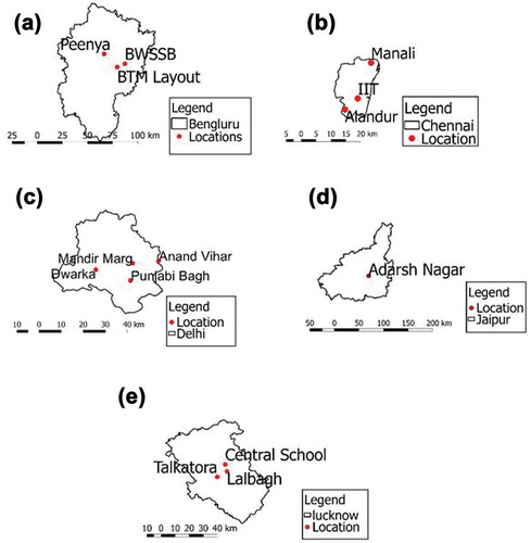
The study area included the data for 14 locations of five capital cities of India, namely, Delhi, Bengaluru, Lucknow, Chennai, and Jaipur. Details of these locations are shown in Table 1. Three out of these five locations, Delhi, Bengaluru, and Chennai, are metropolitan cities with a high population index (Classification of Indian cities 2018), called Tier I cities, and the others are Tier II cities. Locations of these five cities annotated on maps are depicted in Figure 1. Air quality observations for these locations were taken in terms of NO₂ concentrations from air quality monitoring stations installed by the Central Pollution Control Board (CPCB) of the government of India. The method used to extract NO₂ concentrations was a modified Jacob and Hochheiser (Na-arsenite) and chemiluminescence (CPCB 2013) . Further, sampling sites were categorized into three subcategories by government: residential, commercial, and industrial areas, depending upon the land use pattern. Data comprised the raw values of NO₂ concentrations taken every 15 minutes over a period of 3 years, from 2014 through 2016, consisting of a total of 10,38,265 records. Details are given in Table 1.

Table 1. Study area details.

Study number	Location	Description	Latitude	Longitude	Number of records	Area
1	Bengaluru	BTM (Byrasandra, Thavarekere, and Madiwala) Layout	12.91	77.59	76366	Commercial
2	Bengaluru	BWSSB (Bangalore Water Supply and Sewerage Board) Kadabesanahalli	12.93	77.68	77336	Commercial
3	Bengaluru	Peenya	13.027	77.49	70630	Industrial
4	Delhi	Anand Vihar	28.65	77.32	82745	Commercial
5	Delhi	Punjabi Bagh	28.56	77.19	85833	Residential, industrial, and commercial
6	Delhi	Mandir Marg	28.63	77.20	73471	Residential and commercial
7	Delhi	NSIT Dwarka	28.61	77.03	84386	Residential
8	Jaipur	Adarsh Nagar	26.90	75.84	26646	Industrial
9	Lucknow	Lalbagh	26.85	80.94	78307	Commercial
10	Lucknow	Central School	26.88	80.93	75894	Commercial
11	Lucknow	Talkatora District Industries Center	26.84	80.89	56380	Industrial
12	Chennai	Manali	13.16	80.26	89007	Industrial
13	Chennai	Alandur Bus Depot	12.91	80.11	80219	Residential
14	Chennai	IIT	13.01	80.24	81045	Residential

Figure 1. Study area of five megacities of India. (a) Study area of Bengaluru. (b) Chennai. (c) Delhi. (d) Jaipur. (e) Lucknow.

Anomaly detection

Methodological steps followed to extract anomalies is explained further in this section.

• Step 1: Data were checked for missing values and discrepancies. We applied linear interpolation (Han, Pei, and Kamber 2011) method to handle missing values. Data were further transformed using a Z-score normalization method (Han, Pei, and Kamber 2011) to scale the original range of the data. The formula for Z score transformation is expressed as

  (1) $ZScore,{x_i}^{\prime }=\frac{x_i-\mu }{\sigma }$(1)

  where $\mu$ and $\sigma$ are the mean and standard deviation of the vector X = x₁,x₂,..,x_n, respectively. Scaling was done so as to transform the data with 0 mean and 1 standard deviation without changing its distribution.

• Step 2: Data were segmented spatially and temporally to capture the variations in different space–time partitions. Spatial segmentation were performed by separating out data for different locations. Later, temporal segmentation was performed over the data set. The optimal size of temporal partitioning was decided, taking into account less interpartition similarity and more intrapartition similarity among instances. This criteria was satisfied by performing monthly partitions, which according to results showed optimal behavior in terms of daily or yearly partitions.

• Step 3: Proximity of two sequences each of n points, for each partition, was calculated using a distance calculation function. A Euclidean distance measure was used to find out the similarity (reciprocal of distance) between two sequences P_i = (p_i1,p_i2…,p_in) and Q_j = (q_j1,q_j2…,q_jn), defined as per eq 2,

  (2) $d_{ij}=f\left(P_i,Q_j\right)=\sqrt{{\sum }_{k=1}^n{\left(p_{ik}-q_{jk}\right)}^2}$(2)

  where n is the number of points per set.

• Step 4: Feature vectors facilitating pairwise distances for all the sequences over each segmented partition were derived. The primary objective of this step was to reduce the dimensionality of the data and extract the useful information for each of the input sequence. Each feature vector represented the set of pairwise distances among sequences in that partition.

• Step 5: Clustering was performed on the values of derived feature vectors representing pairwise distances, so that similar sequences may be clustered together. Various clustering methods such as hierarchical, density-based, and partitioning-based clustering methods (Han, Pei, and Kamber 2011) can be utilized for clustering of points, representing pairwise distances among sequences. However, in this work, our aim was to exhaustively partition the similar sequences, so a k-means algorithm was selected. The k-means (Han, Pei, and Kamber 2011) is one of the most popular partitioning-based clustering algorithms to cluster the similar points together. There were several reasons to choose k-means specifically. First, it can be used on small data sets easily and converges rapidly given a small data set, which in our case was one feature vector. Second, k-means is the simplest algorithm to work with and implement, given huge amounts of data as well as for small partitions of the data. Third, for our work, we needed to partition the feature vector representing distances based on similarities. To select the optimal value of k, the elbow curve (Han, Pei, and Kamber 2011) method was employed. The k-means resulted in formation of clusters containing sequences for which the behavior was similar in terms of Euclidean distance.

• Step 6: For each of these clusters containing similar sequences, anomalous sequences were segregated, using the difference of each sequence in a cluster with respect to the mean value of all the sequences of that cluster. Anomalies were the points with larger distance from the cluster centers. A sequence P_i^(r) for a spatiotemporal segment r was represented by a feature vector, P_i^(r) = (p_i1^(r),p_i2^(r),…,p_in^(r)), and the mean of all the sequences, $\bar{P}$ ^(r) = ($\overline{p_1}$ ^(r), $\overline{p_2}$ ^(r),…, $\overline{p_n}$ ^(r)), was calculated using eq 3, defined as

  (3) ${\bar{P}}^{\left(r\right)}=\left(\frac{{\sum }_{k=1}^m{p}_{k1}^{\left(r\right)}}{m},\frac{{\sum }_{k=1}^m{p}_{k2}^{\left(r\right)}}{m},\dots ,\frac{{\sum }_{k=1}^m{p}_{kn}^{\left(r\right)}}{m}\right)$(3)

  where m is the number of sequences in a partition r and n is the number of points per sequence. Difference for sequence P_j^(r) was calculated using eq 4, expressed as

  (4) $Diff\left(p_j^{\left(r\right)}\right)=\left(p_{j1}^{\left(r\right)}-\overline{p_1^{\left(r\right)}},p_{j2}^{\left(r\right)}-\overline{p_2^{\left(r\right)}},\dots ,p_{jn}^{\left(r\right)}-\overline{p_n^{\left(r\right)}}\right)$(4)

  Henceforth, to identify the difference of any sequence P_j with respect to mean of all the similar sequences, eq 5 was used:

  (5) $\mathrm{D}\mathrm{i}\mathrm{f}\mathrm{f}\mathrm{w}.\mathrm{r}.\mathrm{t}.\mathrm{m}\mathrm{e}\mathrm{a}\mathrm{n}\mathrm{f}\mathrm{o}\mathrm{r}\mathrm{d}\mathrm{a}\mathrm{y}\left(p_j^{\left(r\right)}\right)={\sum }_{k=1}^n\left(p_{jk}^{\left(r\right)}-\overline{p_k^{\left(r\right)}}\right)$(5)

• Step 7: Gaussian parametric model (Chandola, Banerjee, and Kumar 2009) was employed on these differences to identify the optimal distance after which a point was considered an anomaly. The Gaussian model assumes data to be normal. This model declares all the instances at 3$\sigma$ distance away from the mean, $\mu$, as anomalies. Hence, the sequences outside the $\mu$ +$3\sigma$ region containing 99.7% of the data sequences were identified as anomalies.

Application of Clustering-Based Anomaly Detection Method

The proposed clustering-based anomaly detection (CBAD) method was employed to every daily sequence representing NO₂ concentration at every 15 minutes, over each of the spatiotemporal segments. This process was applied for all the spatiotemporal segments throughout the data. Anomalies for our work were the extreme sequences whose variance, $\sigma$, is quite high or quite low with respect to the mean $\mu$. However, we were interested in only high varying sequence anomalies, that is, anomalous days showing a quite high deviation in concentration of NO₂ with respect to the other days for each month.

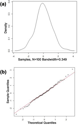
K-means clustering was performed over each of the spatiotemporal segments and means were calculated for each cluster, representing similarly behaving days. Thus, anomalous days depicting extreme NO₂ concentrations with larger deviation from the mean were segregated using the Gaussian method. Figure 2 shows the distribution of 100 randomly selected normalized samples from our data with a p value of 0.7325 for the Shapiro–Wilk normality test (Han, Pei, and Kamber 2011) over alpha 0.05. This suggested that the null hypothesis that data were normal cannot be rejected.

Figure 2. (a) Density plot. (b) Quantile plot of samples.

Our method was able to detect anomalies in almost linear time. Time complexity of k-means is O(n) (Jain, Murty, and Flynn 1999), where n is the number of patterns. Data partitioning has an additional advantage of reducing time complexity, by applying k-means to feature vectors calculated from monthly data segments. Assumptions made for this work were: First, we assumed that data observations considered for our work were standardized and there was no error in taking pollutant readings for each location. Second, we assumed that NO₂ pollutant was independent of other pollutants, that is, that its coexistence with other pollutants was not taken into account.

Clustering

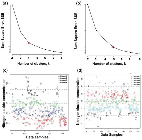
The elbow curve method was used to find the optimal k value by plotting a range of different k values on the X-axis against the error on the Y-axis. Sample elbow curves and the corresponding clusters for two locations obtained over a monthly spatiotemporal segment are illustrated in Figure 3. The elbow is the point in the curve where the decrease in error reduces sharply and an elbow is formed. The value that formed an elbow was selected as the optimal k-value. For instance, this change in Y-axis reduced sharply at point k = 5 in Figure 3b and at point k = 4 in Figure 3a. Hence, 5 and 4 as the numbers of clusters were chosen, and corresponding clusters are depicted in Figure 3c and Figure 3d, respectively.

Figure 3. (a) Elbow curve depicting an elbow at k = 4. (b) Elbow curve depicting an elbow at k = 5. (c) Univariate k-means clustering for optimal k value identified by the elbow curve (a), i.e., k = 4. (d) Univariate k-means clustering for optimal k value identified by the elbow curve (b), i.e., k = 5.

In Table 2 is the cumulative percentage variance explained by k-means clustering of four air quality stations of Delhi. The table suggests that more than 80% of the variance was explained by the k-means for most of the locations, and hence using k-means is justified.

Table 2. Variances and SSE for the four locations of Delhi.

Data-set description	Anand Vihar	Mandir Marg	Punjabi Bagh	Dwarka
Optimal k	4	4	4	4
Var (%)	80.60	69.65	85.25	80.59
SSE	36.28	16.91	32.71	9.77

To verify that most of the anomalies were identified from our method, simple random sampling was performed over a few months from the whole data set, where each sample was drawn without replacement. A sample of 25% of random months, i.e., 3 months, for each of the four locations of a city was taken. For each of these months data visualization was performed and possible anomalies were identified, by segregating sequences that were not similar to most of the sequences. Percentage accuracy for each of these months was calculated as per eq 6:

(6) $Accuracy=1-\frac{S-T}{S}\ast 100$(6)

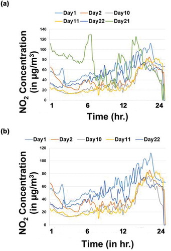
where S is the number of anomalous sequences identified in the sampled data visually and T is the number of anomalous sequences identified from our proposed method. For the samples that were worked on, most of the major sequence anomalies were extracted by our work and the percentage error came out to be approximately less than 10% in most of the cases, which was quite low. For example Figure 4a shows the sample set of days for the month of September at Punjabi Bagh. Accuracy for such a sample came out to be 100%. After removing the anomaly, the set of sampled sequences is shown in Figure 4b. Note the similarity between sequences after removal of anomalies.

Figure 4. Set of randomly sampled days plotted for the month of September 2016, Punjabi Bagh. (a) Dates plotted: 1-9-2016, 10-9-2016, 11-9-2016, 21-9-2016, and 22-9-2016. (b) Removal of anomalous sequence, i.e., 21-9-2016.

Experiments and results

Since this type of study has not been performed in the past for locations in India, annotated data were not available. Additionally, to prove the validity and effectiveness of our method, the model was evaluated over several parameters:

1. What was the performance of our anomaly detection method in comparison to to other methods and data sets?

2. How can we recognize that anomalies extracted by our method were actually anomalies?

3. What about anomalies that were left out?

4. How robust was our method?

Several experiments were performed to answer these questions.

Experiment 1

This experiment was performed in order to validate the extracted anomalies. Our method was compared with two existing baseline methods of anomaly detection. Later, evaluation was done on precision scores and results were extracted.

Baseline methods

Two baseline methods are as follows:

1. Time series anomaly detection method: A combination of seasonal and trend decomposition using the loess and exponential weighted moving average (STL-EWMA) method is a very popular anomaly detection method. Exponential moving average method is an extension of exponential smoothing technique and works well for data streams, as explained in Hochenbaum, Vallis, and Kejariwal (2017). EWMA is a weighted smoothing method, in which each observation is given some weight to calculate the average. This weight is decided based upon the distance with the predicted value, such that nearest values are given more weights than far-away values. Decomposition and smoothing thus segregate anomalies in this method. The formula for EWMA in recursion is given as per eq 7,

   (7) $S_t=\left\{\begin{array}{c}{Y}_t,ift=1\\ \alpha .Y_t+\left(1-\alpha \right).S_{t-1}t>1\end{array}\right.$(7)

   where the coefficient $\alpha$ represents the degree of weighting decrease, for which the value lies between 0 and 1. S_t is the value of the exponential moving average (EMA) at any time period t, which is further given in Hochenbaum, Vallis, and Kejariwal (2017). Y_t is the value at a time period t. Notably, the alpha value is chosen such that optimal results are obtained from all the exhaustive trials between 0 and 1.

2. Statistical method of anomaly detection: Seasonal Hybrid Extreme Studentized Deviate (S-H-ESD) (Hochenbaum, Vallis, and Kejariwal 2017) is a modified form of ESD test method of outlier detection. In this test, the median is used instead of the mean to calculate upper boundaries for detection of outliers. Detailed experiments and results of this method are provided in Hochenbaum, Vallis, and Kejariwal (2017).

Evaluation

Evaluation was performed using two metrics, Precision₁ and Precision₂. The precision score is the probability that the retrieved anomaly is relevant. Precision₁ was the ratio of common anomalies (i.e., anomalies retrieved by our method and by the baseline method) to anomalies retrieved by the baseline method, expressed as a percentage. Precision₂ was the ratio of common anomalies to anomalies retrieved by our method, expressed as a percentage. Formulas for Precision₁ and Precision₂ are given as in eqs 8 and 9:

(8) $Precisio{n}_1=\frac{A\cap B}{A}\ast 100$(8)

(9) $Precisio{n}_2=\frac{A\cap B}{B}\ast 100$(9)

where A was the set of anomalies retrieved from baseline method and B was the set of anomalies retrieved from our method. High Precision₁ denoted that all the anomalies extracted by baseline method were also extracted by our method, while low Precision₁ denoted that very few anomalies were extracted by our method. Hence, high Precision₁ was expected.

Further, high Precision₂ denoted that the anomalies extracted by our method were also the anomalies extracted by baselines, while low Precision₂ suggested that our method was able to extract some more anomalies which were not extracted by baselines.

Our experiments depicted that the method S-H-ESD performed better than STL-EWMA for all the locations with higher scores. The reason for this might be because STL-EWMA was able to identify only abrupt changes in the sequence, and not the anomalous sequence as a whole, while S-H-ESD was able to identify global sequence anomalies quite effectively.

Results

Since results obtained by S-H-ESD method were better than results obtained by STL-EWMA, we considered S-H-ESD as the baseline method for further calculations. Tables 3–6 show the calculated Precision₁ and Precision₂ scores for our method, considering S-H-ESD method as baseline for all the locations of Delhi, Bengaluru, Lucknow, Jaipur, and Chennai for the year 2016. This means that calculations have been done taking A as anomalies from SHESD method and B as our proposed method in calculating precision scores using eqs 8 and 9.

Table 3. Precision₁ (P1) and Precision₂ (P2) scores, representing matches between relevant and retrieved anomalies, for locations Anand Vihar (AV), Punjabi Bagh (PB), Mandir Marg (MM), and Dwarka (Dw.) of Delhi.

	Anand Vihar		Punjabi Bagh		Mandir Marg		Dwarka
	P1	P2	P1	P2	P1	P2	P1	P2
January	–	0	25	100	0	0	100	57.14
February	0	0	100	100	33.33	100	100	33.33
March	–	–	100	50	0	–	100	25
April	100	40	0	0	100	33.33	100	25
May	75	52.86	–	0	–	0	100	33.33
June	100	48.57	50	50	100	33.33	100	33.33
July	100	40	100	40	100	40	100	28.57
August	100	50	0	0	–	0	100	25
September	0	0	0	–	–	0	100	56.67
October	100	48.57	60	42.86	100	66.67	100	100
November	–	–	–	–	0	0	50	50
December	0	0	100	40	–	0	50	100

Table 4. Precision₁ (P1) and Precision₂ (P2) scores, representing matches between relevant and retrieved anomalies, for locations Jaipur, Alandur, IIT, and Chennai.

	Jaipur		Alandur		IIT		Manali
	P1	P2	P1	P2	P1	P2	P1	P2
Jan	50	71.69	72.73	80	–	–	33.33	25
Feb	66.67	80	100	35.29	–	–	66.67	50
Mar	100	7.69	100	27.27	100	30.77	0	0
Apr	62.5	50	100	14.29	66.67	50	80	33.33
May	60	77.27	100	15	66.67	50	–	–
Jun	–	–	–	–	–	–	–	–
Jul	100	71.43	100	28.57	–	–	50	33.33
Aug	–	–	100	14.29	90	6.67	53.33	20
Sep	50	73.33	50	16.67	83.33	55.56	75	27.27
Oct	42.86	66.67	42.86	75	100	14.29	–	–
Nov	0	0	100	12.5	–	–	–	–
Dec	100	11.11	–	–	–	–	0	0

Table 5. Precision₁ (P1) and Precision₂ (P2) scores, representing matches between relevant and retrieved anomalies for Bangalore.

	BTM		BWSSB		Peenya
	P1	P2	P1	P2	P1	P2
Jan	66.67	16.67	100	100	66.67	18.18
Feb	80	50	66.67	66.67	100	33.33
Mar	100	18.18	100	14.29	55.56	50
Apr	85.71	75	100	71.43	75	100
May	57.14	28.57	100	75	50	44.44
Jun	100	100	100	40	100	50
Jul	–	–	–	–	85.71	35.29
Aug	50	16.67	–	–	100	100
Sep	33.33	60	–	–	0	–
Oct	100	100	100	16.67	14.29	20
Nov	100	16.67	0	0	–	–
Dec	100	100	0	0	80	50

Table 6. Precision₁ (P1) and Precision₂ (P2) scores, representing matches between relevant and retrieved anomalies, for Lucknow.

	Central School		Talkatora		Lalbagh
	P1	P2	P1	P2	P1	P2
Jan	–	–	100	81.82	100	7.14
Feb	100	19.05	100	20	100	25
Mar	100	57.14	100	36.67	–	–
Apr	–	–	–	–	100	58.18
May	100	38.33	100	11.11	100	36.67
Jun	100	14.29	100	42.5	100	44.76
Jul	100	39.52	100	34.76	100	45.79
Aug	100	28.57	100	38.33	100	26.32
Sep	100	20	100	43.64	100	20
Oct	–	–	100	15	–	–
Nov	100	66	–	–	100	33.85
Dec	–	–	100	4.17	–	–

Average Precision₁ and Precision₂ scores for four locations of Delhi were calculated as 87.6% and 52.2%. Minimum anomalies were extracted for Mandir Marg, as data contained a lot of missing data sequences. Mean Precision₁ and Precision₂ scores for three locations of Bengaluru were calculated as 82.4% and 52.6%, respectively, which was quite good.

Average Precision₁ and Precision₂ scores for Jaipur were 70.2% and 54.6%, respectively. Similarly, average Precision₁ and Precision₂ scores for all the locations of Chennai were 76.9% and 32.6%, respectively. For Lucknow all the anomalies were retrieved by our method and only 33% is retrieved by existing approaches.

Results showed that, for all the locations, Precision₁ scores were almost always 80%; this means that most of the retrieved values from our method were actually anomalies, for all the cases. Subsequently, Precision₂ scores were almost always greater than or equal to 50%. Precision₂ scores were less because the anomalies extracted by our method were not extracted by baselines. The experiment returns high Precision₁ scores and average Precision₂scores. This implies that all the anomalies retrieved from baselines are retrieved by our method. Thus, we can say that our method performed well.

Experiment 2

To prove that our method performed better than other anomaly detection methods, we applied our anomaly detection method on benchmark data sets and executed the results. To validate the accuracy of our results, comparison with two of the benchmark annotated data sets for anomaly detection was done. The first data set was an activity recognition data set (UCI 2016a) from the UCI repository. Data consisted of accelerometer readings for seven type of activites of 15 users. A data sample of 8640 entries, that is, 24 entries per day, across different users was used. Classes 2, 5, and 6 were rare classes in the data sample. Class distribution of the data set is shown in Table 7. The second data set we have considered was an air quality data set from (UCI 2016b), consisting of several attributes. Tungsten oxide was considered as primary feature to be analyzed. The data set was sampled again for 8640 instances and was further divided into buckets. Anomalies were the values with anomaly score greater than 0.5. Coverage ratios for both these data sets is given in Table 8. Coverage ratio is the number of detected rare classes to that of actual rare classes in the data set (He, Xu, and Deng 2003). From the table it was quite apparent that our method of clustering-based anomaly detection (C-B-AD) outperformed the existing approach of S-H-ESD over both of these data sets in terms of coverage ratios for anomaly detection. Notably, we compared our results with only the S-H-ESD method, because its performance was found to be better than the STL-EWMA as per Hochenbaum, Vallis, and Kejariwal (2017). Similar results were found for our data set, as discussed previously.

Table 7. Class distribution for data sets.

Data-set description	Case	Activity class	Proportion of instances (%)
Activity recognition data set	Common class	1,3,4,7	91.92%
	Rare class	2,5,6	8.08%
Air quality data set	Common class	<0.5	95.79%
	Rare class	>0.5	4.2%

Table 8. Resulted coverage ratios for two benchmark data sets.

Data-set details		Method
Data set	Description	CBAD	SHESD
Data set 1:	Activity recognition	88.33%	80.83%
Data set 2:	Air quality	85.83%	70.56%

Experiment 3

Evaluation metric

To evaluate the performance of our proposed anomaly detection method, two criteria must be satisfied. First, our method should be able to extract out all (or most) of the anomalies. Second, none (or very few) of the anomalous instances should be left out undetected. To satisfy the first criterion, sensitivity or true positive rate was used. Sensitivity percentage (SP) is defined as per eq 10:

(10) $\begin{array}{r}\mathrm{\%}Sensitivity=\frac{Actualanomaliesretreived}{Totalnumberofactualanomalies}\ast 100\end{array}$(10)

To fulfill the second criterion, miss rate (MR) was calculated. Miss rate was the number of anomalous data points classified as normal data point. Miss rate is defined as per eq 11:

(11) $\begin{array}{r}\mathrm{\%}MissRate=\frac{Actualanomaliesnotretreived}{Totalnumberofactualanomalies}\ast 100\end{array}$(11)

In other words, Miss rate ratio = 1 – Sensitivity. For the performance analysis of our work, sensitivity should be as high as possible and miss rate should be as low as possible. The range for these metrics was 0 to 100 in percentage.

Robustness

Robustness was calculated in terms of fallout rate, also called false alarms. The false alarm ratio, FAR, is the number of instances classified as anomalous out of total normal instances (which were not anomalies):

(12) $\begin{array}{r}\mathrm{\%}FalloutRate=\frac{Incorrectlyretrievedasanomalies}{Totalnumberofnormalinstances}\ast 100\end{array}$(12)

False alarms are of no harm, except they minimize the efficiency of any system. To justify that the proposed framework does not classify normal instances as anomalous, the false alarm rate should be low.

Results

Figures 5a and 5b depict the results for all the 14 studied locations. Overall percentage sensitivity for years 2016, 2015, and 2014 was observed to be 72.90%, 79.09%, and 76.65%, respectively, leading to low miss rates for these years, that is, 27.10%, 20.91%, and 23.35%, respectively. In addition, our method was able to observe quite low false alarm rates of 15.03%, 14.72%, and 16.59% for subsequent years. Figure 6 illustrates the fallout rate in percentage for all the locations.

Figure 5. (a) Performance evaluation in terms of sensitivity. (b) Performance evaluation in terms of miss rate.

Figure 6. Fallout rate.

Resulting anomalies

A summary of final results depicting the anomalies extracted for the studied locations is presented in this section. Set of several anomalies extracted for locations of Delhi are shown in Table 9. Further, a demonstration of the anomalies, that is, days with critically high concentrations of NO₂ obtained for all the locations for the year 2016, is given in Table 10. These figures confirm the dependency of anomaly patterns on the space–time information, including variables such as location, day of week, month of year, and so on. A detailed discussion of the reasons for these anomalies is given in the next section.

Table 9. Some common anomalies detected for all the locations of Delhi.

Month	Anand Vihar	Dwarka	Mandir Marg	Punjabi Bagh	Possible reasons
January	–	26-01-2016	05-01-2016	04-01-2016	Traffic and industries
		27-01-2016	04-01-2016	05-01-2016
		30-01-2016		07-01-2016
				30-01-2016
February	–	06-02-2016	06-02-2016	24-02-2016	Traffic suffers due to jat agitation
			20-02-2016
			24-02-2016
March	–	–	–	–
April	27-04-2016	30-04-2016	27-04-2016	26-04-2016	Events
				27-04-2016
May	–	–	–	–
June	03-06-2016	03-06-2016	03-06-2016	03-06-2016	Vehicle congestion, weather, jat agitation
			04-06-2016	04-06-2016
July	24-07-2016				Heavy rains, traffic jams
	25-07-2016
	26-07-2016	19-07-2016	25-07-2016	25-07-2016
	27-07-2016
August	13-08-2016	18-08-2016		15-08-2016	Waterlogging
	30-08-2016			16-08-2016
September	–			–
October	28-10-2016	–	29-10-2016	29-10-2016	Stable burning, Diwali
	29-10-2016		30-10-2016	30-10-2016
				31-10-2016
November–December

Table 10. Anomalies detected for various space–time segments.

Month number	Cluster number	Year	Location	Monthly average NO2 concentration(µg/m^3)	Anomalous NO2 concentration(µg/m^3)	Day
			Alandur
2	3	2016	3-2-2016	14.89	103.19	Wednesday
2	3	2016	8-2-2016	14.89	116.61	Monday
2	3	2016	12-2-2016	14.89	56.19	Friday
9	3	2016	20-9-2016	18.01	110.25	Tuesday
			IIT
9	4	2016	14-9-2016	21.09	199.6	Wednesday
9	4	2016	17-9-2016	21.09	112.68	Saturday
9	4	2016	20-9-2016	21.09	145.8	Tuesday
9	4	2016	21-9-2016	21.09	128.15	Wednesday
			BTM
2	1	2016	1-2-2016	15.58	57.75	Monday
2	1	2016	2-2-2016	15.58	52.13	Tuesday
2	1	2016	3-2-2016	15.58	58.31	Wednesday
			Peenya
2	2	2016	26-2-2016	39.35	154.97	Friday
2	2	2016	27-2-2016	39.35	146.42	Saturday
7	1	2016	1-7-2016	7.9	82.19	Friday
7	1	2016	7-7-2016	7.9	396.22	Thursday
			Central School
2	4	2016	22-2-2016	17.48	97.81	Monday
2	4	2016	23-2-2016	17.48	88.04	Tuesday
7	3	2016	16-7-2016	29.58	361.93	Saturday
			Lalbagh
9	4	2016	1-9-2016	26.64	283.3	Thursday
9	3	2016	12-9-2016	26.64	170.57	Monday
			Talkatora
2	3	2016	13-2-2016	36.52	122.6	Saturday
2	2	2016	6-2-2016	36.52	234.79	Saturday
2	2	2016	11-2-2016	36.52	138.98	Thursday
2	2	2016	24-2-2016	36.52	164.41	Wednesday
			Jaipur
2	1	2016	19-2-2016	34.97	77.73	Friday
2	2	2016	18-2-2016	34.97	101.34	Thursday

Results analysis and discussion

An attempt to validate our results using available sources like print media, Internet, and published articles is made in this section. Subsequently, analyses over several possible reasons for the resulting anomalies for each of the 14 locations of India is investigated.

Location study

Delhi: The Delhi-NCR region is saturated with a variety of industries, including electrical and electronics, home consumables, gems and jewelry, textiles, leather, metals and minerals, plant and machinery, pharmaceutical industries (Delhi 2018), and others. The studied four locations of Delhi are surrounded with various industrial areas. Some of those locations and nearby industrial areas are listed as:

1. Location 1 (Anand Vihar): Patparganj, Jhilmil industrial areas.

2. Location 2 (Punjabi Bagh): Karampura, Kirtinagar, Najafgarh, Mangolpuri industrial areas.

3. Location 3 (Mandir Marg): Rani Jhansi Road.

4. Location 4 (Dwarka): Mayapuri industrial areas.

Hence it was quite difficult to spot any particular industry as the reason for extreme pollutant concentrations. Anand Vihar is a commercial area, and air quality can be deteriorated by domestic activities, vehicular movement, roadside eateries, and open burning of leaves and solid waste (Srivastava et al. 2005). Mandir Marg is almost at the center of Delhi and is one of the busiest intersections of the city. Traffic intersections and fuel stations can cause most of the air pollution in this area. Dwarka is a residential area and air quality can be affected mainly by domestic activities, such as cooking, generator sets for power backup, vehicular movement, roadside eateries, and open burning of leaves and solid waste (Srivastava et al. 2005). In winters, air quality deteriorates further due to increased combustion. Most of the industries are located to the west, south, and southwest of Delhi. Punjabi Bagh lies in west Delhi, near most of the industrial areas. Thus, the primary cause of pollution in Punjabi Bagh might be industries.

Including industrial pollution, other major sources of pollution in Delhi are emissions from coal power plants like in Badarpur and Rajghat, combustion in vehicles, and transport, in addition to agricultural activities, fossil fuel combustion, and so on, constituting approximately 77% of the total pollution caused by NO₂. Other sources for release of NO₂ are biomass and crop burning, fires on dumping grounds and landfills, construction sites, slums, sewage treatment plants, and so on (Gurjar, Ravindra, and Nagpure 2016).

Assuming that most of the normal day-to-day traffic and industrial pollution is constant throughout a month, the occurrence of certain events might be responsible for an increase in concentration of NO₂ on some particular days. Several anomalous days for locations of Delhi are summarized in Table 9. We have further tried to investigate the reasons for occurrence of such anomalies. For example, in the monsoon season, Delhi faces high rain showers every year, leading to massive traffic jams in July (Goyal et al. 2006) and August (Tiwari et al. 2018). During post monsoon season, that is, October and November 2016, there is customarily enormous burning of crop residue in Punjab and Haryana, which leads to a high rise in pollutant concentration in Delhi (Chauhan and Singh 2017; Tiwari et al. 2009).

Nitrogen is among primary pollutants from stable burning, alongwith carbon and particulate matter, because nitrogen compounds such as ammonia are of primary usage in fertilizers. Further, during the period of Diwali, which was in the last week of October 2016, pollution rose to extremely high levels (Dey 2016; Mukherjee et al. 2018). Diwali is the festival of India celebrated every year, in which crackers are burned, causing release of toxic gases in air, including NO₂. Hence, in the first week of November and last week of October, there was a massive increase in pollution (Mandal, Prakash, and Bassin 2012), leading to deteriorating air quality in large parts of Delhi. Major preventive steps were suggested by the government (Dholakia et al. 2013) to take control of this.

For anomalous days of February, we arrived at several possible reasons (Shah 2017), such as increased vehicle congestion (Liu et al. 2016), weather (Chowdhury et al. 2017), and others. from studied sources. Further, December to February is the winter season in Delhi. Winters experience more pollution every year than the summers (Tiwari et al. 2018).

For June 2016, significantly, there were continued events of fire (ToI 2018) during Jat agitation near NH-1, the Delhi to Panipat route. Massive properties were burned during this event, leading to traffic congestion on roads on which vehicles were diverted. Combustion is also one of the prime reasons for an increase in nitrogen compounds (Chowdhury et al. 2017). Essentially, we have tried to find maximum possible causes based upon research. However, there might be some other events too, in addition to those identified and discussed in this work. It is impossible to identify each and every one of them.

Lucknow: Lucknow is the capital city of Uttar Pradesh state and the second largest city of North India (Lawrence and Fatima 2014), known for its cultural heritage. Lucknow is a well-known hub for small-scale industries like handicrafts, handwoven clothes, earthen pots, and so on. Out of three stations, Lalbagh and Talkatora showed high concentrations of NO₂ than the Central School on an average, because of nearby industrial areas; popular among them is the Nadarganj industrial area. In addition to industrial pollution, major sources of NO₂ pollution in Lucknow are the construction sites and burning of fossil fuels in vehicles, and burning activities in households and industries. Thus, sources of pollution from NO₂ in Lucknow are less than the other pollutants such as particulate matter and oxides of carbon. The climate of Lucknow is subtropical and varies from humid summers (March–May) and mild winters (December–February). Winter months are critical for air pollution due to climatic conditions (Tiwari et al. 2018), which is the reason for high levels of pollution during winter season.

In, Lucknow, after energy generation and industries, residential areas are the third largest contributors of pollution (Guo et al. 2017). However, for NO₂, we noticed major anomalies during October, and a reason for such anomalies could be the Diwali festival, which is celebrated with rejoicing all over residential areas of Lucknow every year.

Major residential areas lie near Central School. Furthermore, Lalbagh is a commercial area, so no such anomalies were detected. Most of the pollution in Talkatora comes from industries, but there is some residential area near Talkatora, and this might be the another cause of anomalies.

Besides this, other possible reasons for anomalies could be lots of construction work of flyovers and underground metros, causing traffic jams (Gupta and Arya 2016; Times 2016). Note that all the stations of Lucknow were not at quite a distance, and hence some common anomalies for each of these stations were found.

Bengaluru: Bengaluru is known as one of the eminent technology capitals of India, with a high population, where a large number of people work in the information technology (IT) industry. Traffic jams are a major worry during the whole year for most parts of the congested commercial areas of Bengaluru. According to studies, vehicle emission and dust constitute up to 68% of the pollution in the city (Guttikunda, Goel, and Pant 2014), in addition to pollution from the deisel power station at Yelahanka and diesel generator sets. Hence, the main source of NO₂ is vehicle pollution in the city (Nagendra, Venugopal, and Jones 2007; Sabapathy 2008). The climate of Bengaluru remains moderate throughout the year, including monsoon season from July to October. Bengaluru suffers from heavy rains during the monsoon season, causing waterlogging in most of the urban areas. Since most of the population in Bengaluru is a working population, urban areas remain crowded with vehicles during this time (Nagendra, Venugopal, and Jones 2007; Sabapathy 2008; Wang et al. 2017). However, during the rest of the year, highlighted reasons for high pollution could be industries and construction work (Matters 2016; Thakur 2017). BTM is the commercial area of Bengaluru with limited anomalies and BWSSB is a residential area with very few anomalies. Peenya is an industrial area, so we can see that almost all the months see a rising air pollution (Nagendra, Venugopal, and Jones 2007), and hence more anomalies than BTM and BWSSB.

Jaipur: Pink city Jaipur is the capital of Rajasthan state in India and is one of the mega cities of the state. Jaipur is famous for its cultural heritage sites; hence the major income source in Jaipur is the tourism industry. Furthermore, Jaipur is quite famous for its small-scale industry of textiles, carpets, gemstone cutting, and so on (Taknet 2016). Jaipur is also famous for its mining activities of minerals such as limestone, mica, and others at nearby locations. There are varied industrial units, such as manufacturing, textiles, dye, food, chemical, and so on (Singh and Chandel 2006), causing industrial pollution. During October, air pollution was also generated from Diwali festival, in which crackers are burst all over residential areas of Rajasthan including Jaipur, contributing to pollution. Most of the air pollution in Jaipur comes from vehicles, industries, and households (Jawaid et al. 2017).

Chennai: Chennai is the capital of Tamil Nadu state, located on the coast of the Bay of Bengal. Chennai is among the top metropolitan cities of India in terms of economy. Chennai is one of the largest industrial and commercial sectors in India. The industrial base in Chennai includes industries like automobiles, IT industry, hardware manufacturing, petrochemicals, aerospace manufacturing, health care industries, and others (Srivastava et al. 2014). These industries generate tons of waste every year. Burning of such waste causes release of harmful gases into the air. In addition to industrial pollution and burning of industrial wastes, road dust and traffic jams (Guttikunda, Goel, and Pant 2014) have also been identified as a major cause of air pollution in urban areas of Chennai. Furthermore, thermal power plants at Ennore, Athipattu, and Vallur further degrade the air quality levels. The climate of Chennai is mostly hot, with heavy rainfall from September to November, and medium rainfall from June to August. During rains, the problem of traffic jams is further increased for stations near commercial areas. For our work, Alandur and Indian Institutes of Technology (IIT) locations are residential areas, while Manali is surrounded by industries. Manali is quite distant from these two locations.

Comparative analysis

Summarized analyses of primary reasons contributing to anomalies considering the economies of the studied urban cities are given in Table 11. Details about the five cities such as annual rainfall (Department 2011), population (Government 2011), and area (Atlas 2018; Maps of India 2015) are obtained from data provided by the government of India. Table 11 summarizes the economies of the locations, as well as the major pollution sources in the cities.

Table 11. Summary of analysis of various urban localities considering economies of the cities.

City	Description	Major industries	Other primary pollution sources
Delhi	Climate: humid to semi-arid subtropical Population: 46 million Area: 34,144 km^2 Annual rainfall: 54.23 in Season: hot summers, cool winters, humid monsoons	Electrical and electronics, home consumables, gems and jewelery, textiles, leather, metals and minerals, plant and machinery, pharmaceutical industries	Vehicular and industrial emissions, construction work, crop burning, fires in dumping ground, fossil fuel combustion, thermal power plants, etc.
Bengaluru	Climate: tropical savannah Population: 12.3 million Area: 8,005 km^2 Annual rainfall: 83.5 in Season: wet and dry	IT software industry hub, aerospace, manufacturing public sector, aviation and space technology units. biotechnology firms, etc.	Dust, traffic congestion in commercial areas for most times of the year, including waterlogging during rains, industrial pollution, etc.
Lucknow	Climate: humid subtropical Population: 2.8 million Area: 2,528 km^2 Annual rainfall: 54.46 in Season: humid summers and mild winters	Small scale industries like handicrafts, clothes, etc., aerospace, pharmaceuticals, chemical, housing, sugarcane, dyer breweries, etc.	Agriculture activities, construction sites, combustion in vehicles, combustion of fossils in industries, household activities, etc.
Chennai	Climate: tropical wet and dry Population: 8 million Area: 1,189 km^2 Annual rainfall: 77.23 in Season: rainy and dry	Automobiles, IT industry, hardware manufacturing, petrochemical, aerospace and health care industries, etc.	Electricity generation from power plants, dust, traffic in commercial areas, burning of huge industrial wastes including plastics
Jaipur	Climate: hot semiarid Population: 3.1 million Area: 484.6 km^2 Annual rainfall: 48.7 in Season: hot and humid	Small-scale industry of textiles, carpets, gemstone cutting, etc.; mining of minerals, e.g. limestone, mica, etc.; manufacturing, food, chemicals, etc.	Industrial pollution, traffic from tourism, mining of minerals, and household activities

Conclusion

The study of concentrations of pollutants in atmosphere is paramount to a perspective on human health, so that preventive measures can be taken. This study investigated the presence of extremely high concentrations of NO₂ in air. The proposed anomaly detection method employed a hybrid proximity- and clustering-based approach to extract anomalies from the air quality data in terms of concentrations of NO₂. Data samples obtained for 14 residential, commercial, and industrial zones of five metropolitan cities of India are studied. Days with anomalous NO₂ concentrations for these locations are extracted. To validate the effectiveness and efficiency of our proposed method, several experiments are carried out. Furthermore, comparison of proposed approach with existing anomaly detection methods of STL-EWMA and S-H-ESD and several benchmark data sets are done. Results are evaluated extensively in terms of various metrics including sensitivity, miss rate, and fallout rate. Empirical evidence showed that our method outperformed the existing methods of anomaly detection. Additionally, a detailed study over the reasons causing anomalies at various locations is presented. In the future we plan to implement this work on various other pollutants.

Acknowledgment

The authors thank the China Section of the Air & Waste Management Association for the generous scholarship they received to cover the cost of page charges, and to make the publication of this paper possible.

Additional information

Notes on contributors

Apeksha Aggarwal

Apeksha Aggarwal is working as a research scholar at Department of Computer Science and Engineering, Indian Institute of Technology Roorkee, India. Her areas of interest are: Data Mining, Time Series Data Mining, Anomaly detection.

Durga Toshniwal

Durga Toshniwal is currently working as Professor at Department of Computer Science and Engineering, Indian Institute of Technology Roorkee, India. Her areas of interest are: Data Mining and Big Data, Artificial Intelligence, and Machine Learning, Time Series Data Mining, Privacy Preserving Data Mining, Anomaly detection, Data Stream mining.

References

- Aggarwal, A., and D. Toshniwal. 2018a. Predicting particulate matter for assessing air quality in Delhi using meteorological features. Paper presented at International Conference on Computational Science and Its Applications, 623–38. Cham: Springer.
- Aggarwal, A., and D. Toshniwal. 2018b. Visibility prediction in Urban localities using clustering. Paper presented at International Conference on Advances in Computing and Data Sciences, 370–79. Singapore: Springer.
- Aggarwal, A., and D. Toshniwal. 2018c. Spatio-temporal frequent itemset mining on web data. Paper presented at EEE International Conference on Data Mining Workshops, 1160–65. Singapore: IEEE.
- Agrawal, M., B. Singh, M. Rajput, F. Marshall, and J. Bell. 2003. Effect of air pollution on peri-urban agriculture: A case study. Environ. Pollut. 126 (3):323–29. doi:10.1016/s0269-7491(03)00245-8.
- Aguilera, I., M. Guxens, R. Garcia-Esteban, T. Corbella, M. Nieuwenhuijsen, C. Foradada, and J. Sunyer. 2009. Association between GIS-BASED EXPOSURE to Urban air pollution during pregnancy and birth weight in the INMA Sabadell Cohort. Environ. Health Perspect. 117 (8):1322–27. doi:10.1289/ehp.0800256.
- Araki, S., H. Shimadera, K. Yamamoto, and A. Kondo. 2017. Effect of spatial outliers on the regression modelling of air pollutant concentrations: A case study in japan. Atmos. Environ. 153:83–93. doi:10.1016/s0269-7491(03)00245-8.
- Araujo, R. D. A., A. L. Oliveira, and S. Meira. 2017. On the problem of forecasting air pollutant concentration with morphological models. Neurocomputing. 265:91–104. doi:10.1016/j.neucom.2017.01.107.
- Atlas, W. 2018. Metro cities of india. Accessed March 2018, 23. https://www.worldatlas.com/articles/metro-cities-in-india.html.
- Azid, A., H. Juahir, M. E. Toriman, M. K. A. Kamarudin, A. S. M. Saudi, C. N. C. Hasnam, N. A. A. Aziz, F. Azaman, M. T. Latif, S. F. M. Zainuddin, et al. 2014. Prediction of the level of air pollution using principal component analysis and artificial neural network techniques: A case study in malaysia. Water Air Soil Pollut. 225 (8):2063. doi:10.1007/s11270-014-2063-1.
- Bai, X. X., J. Dong, X. G. Rui, H. F. Wang, and W. J. Yin (2017, May 18). Very short-term air pollution forecasting. US Patent App. 14/939, 522.
- Baklanov, A., A. Rasmussen, B. Fay, E. Berge, and S. Finardi. 2002. Potential and shortcomings of numerical weather prediction models in providing meteorological data for urban air pollution forecasting. Water Air Soil Pollut. 2 (5–6):43–60. doi:10.1007/978-94-010-0312-4_4.
- Bay, S. D., and M. Schwabacher. 2003. Mining distance-based outliers in near linear time with randomization and a simple pruning rule. Paper presented at Proceedings of the ninth ACM SIGKDD international conference on Knowledge discovery and data mining, 29–38. Washington, DC: ACM.
- Briggs, D. J., S. Collins, P. Elliott, P. Fischer, S. Kingham, E. Lebret, K. Pryl, H. Van Reeuwijk, K. Smallbone, and A. Van Der Veen. 1997. Mapping urban air pollution using gis: A regression-based approach. Int. J. Geogr. Inf. Sci. 11 (7):699–718. doi:10.1080/136588197242158.
- Chaabouni, S. 2016. Modeling and forecasting 3e in eastern asia: A comparison of linear and nonlinear models. Qual. Quant. 50 (5):1993–2008. doi:10.1007/s11135-015-0247-4.
- Chandola, V., A. Banerjee, and V. Kumar. 2009. Anomaly detection: A survey. ACM Comput. Surv. 41 (3):15. doi:10.1145/1541880.1541882.
- Chandola, V., A. Banerjee, and V. Kumar. 2012. Anomaly detection for discrete sequences: A survey. IEEE Trans. Knowl. Data Eng. 24 (5):823–39. doi:10.1109/tkde.2010.235.
- Chauhan, A., and R. P. Singh. 2017. Poor air quality and dense haze/smog during 2016 in the Indo-Gangetic plains associated with the crop residue burning and Diwali festival. Paper presented at Geoscience and Remote Sensing Symposium (IGARSS), 2017 IEEE International, Fort Worth, Texas, 6048–51. IEEE.
- Cheboli, D. 2010. Anomaly detection of time series. Dissertations and Theses, 2010.
- Chowdhury, S., S. Dey, S. N. Tripathi, G. Beig, A. K. Mishra, and S. Sharma. 2017. Traffic intervention policy fails to mitigate air pollution in megacity delhi. Environ. Sci. Policy. 74:8–13. doi:10.1007/s11135-012-9749-5.
- Classification of Indian cities (2018). Classification of Indian cities. Accessed November 2018, 30. https://en.wikipedia.org/wiki/Classification_of_Indian_cities
- CPCB 2013. Ambient Air Quality Data of Delhi-NCR. Accessed November 2018, 30. http://cpcb.nic.in/NGT/AirQualitydataDelhiNCRDecember2017.pdf.
- Crouse, D. L., M. S. Goldberg, and N. A. Ross. 2009. A prediction-based approach to modelling temporal and spatial variability of traffic-related air pollution in montreal, canada. Atmos. Environ. 43 (32):5075–84. doi:10.1016/j.envsci.2017.04.018.
- Delhi, F. 2018. Industries in delhi. Accessed March 2018, 23. http://www.focusdelhi.com/business-and-finance/industries-in-delhi.html.
- Department, I. M. 2011. Customized rainfall information system (cris). Accessed February 2018, 22. http://hydro.imd.gov.in/hydrometweb/(S(w3zmi1rxdkiaafihre5eikab))/DistrictRaifall.aspx.
- Dey, P. “Diwali: A smog-mare for the Indian capital.” South Asia@ LSE 2016.
- Dholakia, H. H., P. Purohit, S. Rao, and A. Garg. 2013. Impact of current policies on future air quality and health outcomes in delhi, india. Atmos. Environ. 75 (2013):241–48. doi:10.1016/j.atmosenv.2013.04.052.
- Donnelly, A., B. Misstear, and B. Broderick. 2015. Real time air quality forecasting using integrated parametric and non-parametric regression techniques. Atmos. Environ. 103:53–65. doi:10.1016/j.atmosenv.2014.12.011.
- Effiong, E. L. 2018. On the urbanization-pollution nexus in africa: A semiparametricanalysis. Qual. Quant. 52 (1):445–56. doi:10.1007/s11135-017-0477-8.
- Fanger, P. O. 1988. Introduction of the olf and the decipol units to quantify air pollution perceived by humans indoors and outdoors. Energy Build. 12 (1):1–6. doi:10.1016/0378-7788(88)90051-5.
- Feng, X., Q. Li, Y. Zhu, J. Hou, L. Jin, and J. Wang. 2015. Artificial neural networks forecasting of pm2. 5 pollution using air mass trajectory based geographic model and wavelet transformation. Atmos. Environ. 107:118–28. doi:10.1016/j.atmosenv.2015.02.030.
- Government, I. 2011. Open govenment data. Accessed February 2018, 22. https://data.gov.in/.
- Goyal, S., S. Ghatge, P. Nema, and S. Tamhane. 2006. Understanding urban vehicular pollution problem vis-a-vis ambient air quality case study of a megacity (delhi, india). Environ. Monit. Assess. 119 (1–3):557–69. doi:10.1007/s10661-005-9043-2.
- Guo, H., S. H. Kota, S. K. Sahu, J. Hu, Q. Ying, A. Gao, and H. Zhang. 2017. Source apportionment of pm2. 5 in north india using source-oriented air quality models. Environ. Pollut. 231:426–36. doi:10.1016/j.envpol.2017.08.016.
- Gupta, V., and A. K. Arya. 2016. Demonstrating urban pollution using heavy metals in road dusts from lucknow city, uttar pradesh, india. Environ. Conserv. J. 17 (1&2):137–46.
- Gurjar, B., K. Ravindra, and A. S. Nagpure. 2016. Air pollution trends over indian megacities and their local-to-global implications. Atmos. Environ. 142:475–95. doi:10.19070/2330-0027-160007.
- Guttikunda, S. K., R. Goel, and P. Pant. 2014. Nature of air pollution, emission sources, and management in the indian cities. Atmos. Environ. 95:501–10. doi:10.1016/j.atmosenv.2014.07.006.
- Han, J., J. Pei, and M. Kamber. 2011. Data mining: Concepts and techniques. USA: Elsevier.
- He, Z., X. Xu, and S. Deng. 2003. Discovering cluster-based local outliers. Pattern Recognit. Lett. 24 (9–10):1641–50. doi:10.1016/s0167-8655(03)00003-5.
- Hochenbaum, J., O. S. Vallis, and A. Kejariwal. 2017. Automatic anomaly detection in the cloud via statistical learning. arXiv preprint. arXiv:1704.07706.
- Hwang, J.-H., and S.-H. Yoo. 2014. Energy consumption, co 2 emissions, and economic growth: Evidence from indonesia. Qual. Quant. 48 (1):63–73. doi:10.1007/s11135-012-9749-5.
- Ibarra-Berastegi, G., A. Elias, A. Barona, J. Saenz, A. Ezcurra, and J. D. de Argandona. 2008. From diagnosis to prognosis for forecasting air pollution using neural networks: Air pollution monitoring in bilbao. Environ. Model Softw. 23 (5):622–37. doi:10.1016/j.envsoft.2007.09.003.
- Irfan, M., and K. Shaw. 2017. Modeling the effects of energy consumption and urbanization on Environment Pollution in south asian countries: A nonparametric panel approach. Qual. Quant. 51 (1):65–78. doi:10.1016/j.envsoft.2007.09.003.
- Jain, A. K., M. N. Murty, and P. J. Flynn. 1999. Data clustering: A review. ACM Comput. Surv. 31 (3):264–323. doi:10.1145/331499.331504.
- Jawaid, M., M. Sharma, S. Pipralia, and A. Kumar. 2017. City prole: Jaipur. Cities. 68:63–81. doi:10.1016/j.cities.2017.05.006.
- Karppinen, A., J. Kukkonen, T. Elolahde, M. Konttinen, T. Koskentalo, and E. Rantakrans. 2000. A modelling system for predicting urban air pollution: Model description and applications in the helsinki metropolitan area. Atmos. Environ. 34 (22):3723–33. doi:10.1016/s1352-2310(00)00074-1.
- Klink, A., L. Polechonska, A. Ceg Lowska, and A. Stankiewicz. 2016. Typha latifolia (broadleaf cattail) as bioindicator of different types of pollution in aquatic ecosystemsapplication of self-organizing feature map (neural network). Environ. Sci. Pollut. Res. 23 (14):14078–86. doi:10.1007/s11356-016-6581-9.
- Knox, E. M., and R. T. Ng. 1998. Algorithms for mining distancebased outliers in large datasets. Paper presented at Proceedings of the international conference on very large data bases, 392–403.New York, NY: Citeseer.
- Kumar, P., S. Jain, B. Gurjar, P. Sharma, M. Khare, L. Morawska, and R. Britter. 2013. New directions: Can a blue sky return to indian megacities? Atmos. Environ. 71:198–201. doi:10.1016/j.atmosenv.2013.01.055.
- Kumar, R., and A. E. Joseph. 2006. Air pollution concentrations of pm2. 5, pm10 and no2 at ambient and kerbsite and their correlation in metro city mumbai. Environ. Monit. Assess. 119 (1–3):191–99. doi:10.1016/j.atmosenv.2013.01.055.
- Kurt, A., B. Gulbagci, F. Karaca, and O. Alagha. 2008. An online air pollution forecasting system using neural networks. Environ. Int. 34 (5):592–98. doi:10.1016/j.envint.2007.12.020.
- Latza, U., S. Gerdes, and X. Baur. 2009. Effects of nitrogen dioxide on human health: Systematic review of experimental and epidemiological studies conducted between 2002 and 2006. Int. J. Hyg. Environ. Health. 212 (3):271–87. doi:10.1016/j.ijheh.2008.06.003.
- Lawrence, A., and N. Fatima. 2014. Urban air pollution & its assessment in lucknow citythe second largest city of north india. Sci. Total Environ. 488:447–55. doi:10.1016/j.ijheh.2008.06.003.
- Liu, C., B. H. Henderson, D. Wang, X. Yang, and Z.-R. Peng. 2016. A land use regression application into assessing spatial variation of intra-urban fine particulate matter (pm2. 5) and nitrogen dioxide (no2) concentrations in city of shanghai, china. Sci. Total Environ. 565:607–15. doi:10.1016/j.scitotenv.2016.03.189.
- Liu, Z., K. Cheng, H. Li, G. Cao, D. Wu, and Y. Shi. 2018. Exploring the potential relationship between indoor air quality and the concentration of airborne culturable fungi: A combined experimental and neural network modeling study. Environ. Sci. Pollut. Res. 25 (4):3510–17. doi:10.1007/s11356-017-0708-5.
- Mandal, P., M. Prakash, and J. Bassin. 2012. Impact of diwali celebrations on urban air and noise quality in delhi city, india. Environ. Monit. Assess. 184 (1):209–15. doi:10.1007/s11356-017-0708-5.
- Maps of India. 2015. Maps of india. Accessed March2018, 23. https://www.mapsofindia.com/maps/cities/cities-in-india.html.
- Matters, C. 2016. A road where construction never ends, nor do traffc snarls. Accessed February 2018, 22. http://bengaluru.citizenmatters.in/flyovers-construction-on-orr-traffic-congestion-in-bangalore-8848.
- Michaelides, S., D. Paronis, A. Retalis, and F. Tymvios. 2017. Monitoring and forecasting air pollution levels by exploiting satellite, ground-based, and synoptic data, elaborated with regression models. Advances Meteorol. 2017: doi: 10.1155/2017/2954010.
- Mukherjee, T., A. Asutosh, S. K. Pandey, L. Yang, P. P. Gogoi, A. Panwar, and V. Vinoj. 2018. Increasing potential for air pollution over megacity new delhi: A study based on 2016 diwali episode. Aerosol. Air Qual. Res. 18:2510–18. doi:10.4209/aaqr.2017.11.0440.
- Nagendra, S. S., and M. Khare. 2005. Modelling urban air quality using artificial neural network. Clean Technol. Environ. Policy. 7 (2):116–26. doi:10.4209/aaqr.2017.11.0440.
- Nagendra, S. S., K. Venugopal, and S. L. Jones. 2007. Assessment of air quality near traffic intersections in bangalore city using air quality indices. Transp. Res. D Transp. Environ. 12 (3):167–76. doi:10.1016/j.trd.2007.01.005.
- Niska, H., T. Hiltunen, A. Karppinen, J. Ruuskanen, and M. Kolehmainen. 2004. Evolving the neural network model for forecasting air pollution time series. Eng. Appl. Artif. Intell. 17 (2):159–67. doi:10.1016/j.engappai.2004.02.002.
- Pandey, J. S., R. Kumar, and S. Devotta. 2005. Health risks of no2, spm and so2 in delhi (india). Atmos. Environ. 39 (36):6868–74. doi:10.1016/j.atmosenv.2005.08.004.
- Perez, P., and J. Reyes. 2001. Prediction of particulate air pollution using neural techniques. Neural Comput. Appl. 10 (2):165–71. doi:10.1007/s005210170008.
- Prasad, K., A. K. Gorai, and P. Goyal. 2016. Development of anfis models for air quality forecasting and input optimization for reducing the computational cost and time. Atmos. Environ. 128:246–62. doi:10.1016/j.atmosenv.2016.08.012.
- Rahman,Lee, and Latif, et al. 2015. Artificial neural networks and fuzzpp.y time series forecasting: An application to air quality. Qual. Quant. 49 (6):2633–47. doi:10.1007/s11135-014-0132-6.
- Ramaprasad, A., A. Sánchez-Ortiz, and T. Syn. 2017. A unified definition of a smart City. Paper presented at International Conference on Electronic Government: 13–24. Cham, St. Petersburg, Russia: Springer.
- Ramaswamy, S., R. Rastogi, and K. Shim. 2000. Efficient algorithms for mining outliers from large data sets. Paper Presented at ACM Sigmod Record. 29 (2):427–38. ACM. doi:10.1145/335191.
- Rosenfeld, D. 2000. Suppression of rain and snow by urban and industrial air pollution. Science. 287 (5459):1793–96. doi:10.1126/science.287.5459.1793.
- Ryan, P. H., and G. K. LeMasters. 2007. A review of land-use regression models for characterizing intraurban air pollution exposure. Inhal. Toxicol. 19 (1):127–33. doi:10.1080/08958370701495998.
- Sabapathy, A. 2008. Air quality outcomes of fuel quality and vehicular technology improvements in bangalore city, india. Transp. Res. D Transp. Environ. 13 (7):449–54. doi:10.1016/j.trd.2008.09.001.
- Saidi, K., and S. Hammami. 2016. Economic growth, energy consumption and carbone dioxide emissions: Recent evidence from panel data analysis for 58 countries. Qual. Quant. 50 (1):361–83. doi:10.1016/j.trd.2008.09.001.
- Shah, K. M. 2017. Dealing with violent civil protests in India. New Delhi, India: Report.
- Singh, V., and C. S. Chandel. 2006. Analytical study of heavy metals of industrial effluents at jaipur, rajasthan (india). J. Environ. Sci. Eng. 48 (2):103–08.
- Srivastava, A., A. Joseph, S. Patil, A. More, R. Dixit, and M. Prakash. 2005. Air toxics in ambient air of delhi. Atmos. Environ. 39 (1):59–71. doi:10.1016/j.atmosenv.2004.09.053.
- Srivastava, D., K. Shanmugam, K. K. Kumar, and M. Saripalle 2014. Fiscal instruments for climate friendly industrial development in tamil nadu. Report.
- Stripling, E., B. Baesens, B. Chizi, and S. Vanden Broucke. 2018. Isolation-based conditional anomaly detection on mixed-attribute data to uncover workers’ compensation fraud. Decis. Support Syst. Report. doi: 10.1016/j.dss.2018.04.001.
- Taknet, D. K. 2016. Jaipur: Gem of India. IntegralDMS. Jaipur, India: Report.
- Thakur, A. 2017. Study of ambient air quality trends and analysis of contributing factors in bengaluru, india. Orient. J. Chem. 33 (2):1051–56. doi:10.13005/ojc/330265.
- Times, N. 2016. Possible traffic jam at hazratganj. Accessed January 2018, 30. https://navbharattimes.indiatimes.com/metro/lucknow/development/possible-traffic-jam-at-hazratganj/articleshow/53902624.cms.
- Tiwari, S., G. Pandithurai, S. Attri, A. Srivastava, V. Soni, D. Bisht, V. A. Kumar, and M. K. Srivastava. 2015. Aerosol optical properties and their relationship with meteorological parameters during wintertime in delhi, india. Atmos. Res. 153:465–79. doi:10.1016/j.atmosres.2014.10.003.
- Tiwari, S., A. K. Srivastava, D. S. Bisht, T. Bano, S. Singh, S. Behura, M. K. Srivastava, D. Chate, and B. Padmanabhamurty. 2009. Black carbon and chemical characteristics of pm 10 and pm 2.5 at an urban site of north india. J. Atmos. Chem. 62 (3):193–209. doi:10.1007/s10874-010-9148-z.
- Tiwari, S., A. Thomas, P. Rao, D. Chate, V. Soni, S. Singh, S. Ghude, D. Singh, and P. K. Hopke. 2018. Pollution concentrations in delhi india during winter 2015-16: A case study of an odd-even vehicle strategy. Atmos. Pollut. Res. 9 (6):1137–45. doi:10.1016/j.apr.2018.04.008.
- ToI. 2018. Accessed January 2018, 30. https://timesofindia.indiatimes.com/city/noida/Jat-quota-stir-Dadri-tension-keep-Delhi-NCR-on-edge/articleshow/52612333.cms.
- UCI. 2016a. Uci machine learning repository: Activity recognition from single chest-mounted accelerometer data set. Accessed February2018, 13. https://archive.ics.uci.edu/ml/datasets/Activity+Recognition+from+Single+Chest-Mounted+Accelerometer.
- UCI. 2016b. Uci machine learning repository: Air quality data set. Accessed February 2018, 13. https://archive.ics.uci.edu/ml/datasets/Air+quality.
- Wang, Y., L. Yang, S. Han, C. Li, and T. Ramachandra. 2017. Urban co2 emissions in xian and bangalore by commuters: Implications for controlling urban transportation carbon dioxide emissions in developing countries. Mitig. Adapt. Strateg. Glob. Chang. 22 (7):993–1019. doi:10.1007/s11027-016-9704-1.
- Weng, Q., and S. Yang. 2006. Urban air pollution patterns, land use, and thermal landscape: An examination of the linkage using gis. Environ. Monit. Assess. 117 (1–3):463–89. doi:10.1007/s10661-006-0888-9.
- Yildirim, Y., and M. Bayramoglu. 2006. Adaptive neuro-fuzzy based modelling for prediction of air pollution daily levels in city of zonguldak. Chemosphere. 63 (9):1575–82. doi:10.1016/j.chemosphere.2005.08.070.
- Zhang, H., Y. Zheng, and Y. Yu. 2018. Detecting urban anomalies using multiple spatio-temporal data sources. Proceedings of the ACM on interactive. Mobile, Wearable Ubiquitous Technol. 2 (1):54.
- Zhang, Y., M. Bocquet, V. Mallet, C. Seigneur, and A. Baklanov. 2012. Real-time air quality forecasting, part i: History, techniques, and current status. Atmos. Environ. 60:632– 55. doi:10.1016/j.atmosenv.2012.06.031.
- Zheng, Y., F. Liu, and H.-P. Hsieh. 2013. “U-Air: When urban air quality inference meets big data.” Paper presented at Proceedings of the 19th ACM SIGKDD international conference on Knowledge discovery and data mining, Chicago, 1436–44. ACM.