Assessment of tropospheric ozone at an industrial site of Chennai megacity

ABSTRACT

This paper presents the temporal variation in surface-level ozone (O₃) measured at Gummidipoondi near Chennai, Tamilnadu. The site chosen for the present study has high potential for ozone generation sources, such as vehicular traffic and industrial activities. The site is also located near a hazardous waste management facility. The key sources of nitrogen oxides (NO_x), which are considered to be an important precursor of O₃, include hazardous waste incineration, trucks bringing the hazardous wastes, and vehicles plying on the nearby National Highway 16 (NH 16). The measurements clearly showed diurnal variation, with maximum values observed during the noon hours and minimum values observed when solar radiation was less. The data showed a marked seasonal variation in O₃, with the highest hourly average O₃ concentration (497.2 µg/m³) in the summer season. Consequently, in order to identify the long-range transport sources adding to the increased O₃ levels, backward trajectories were computed using the Hybrid Single Particle Lagrangian Integrated Trajectory (HYSPLIT) model. It was found that the polluted air mass originated from the Southeast Asian region and the Indo-Gangetic Plain. The polluted air mass, which advected large amounts of carbon monoxide (CO) plumes, was analyzed using the Measurement of Pollution in the Troposphere (MOPITT) retrievals. The correlations of O₃ with temperature (r = 0.746; P < 0.01) and solar radiation (r = 0.751; P < 0.01) were strongly positive, and that with NO_x was found to be negative. Stronger correlation of O₃ with NO_x was observed during pre-monsoon months (r = 0.627; P < 0.01) and following hours of photochemical reactions. There were substantial differences in concentrations between weekdays and weekends, with higher nitric oxide (NO) and nitrogen dioxide (NO₂), but lower O₃, concentrations on weekdays. A substantial weekday-weekend difference in O₃, which was higher on weekends, appears to be attributable to lower daytime traffic activity and hence reduced emissions of NO_x to a “NO_x-saturated” atmosphere.

Implications: The assessment of ground-level ozone in an industrial area with hazardous waste management facility is very important, as there is high possibility for more generation of tropospheric ozone. Since the location of the study area is coastal, wind plays a major role in O₃ transportation; hence, the effects of wind speed and wind direction have been studied in different seasons. When compared with the other studies carried out in different places across India, the present study area has recorded much greater O₃ mixing ratio. This study can be useful for setting up control strategies in such industrial areas.

Introduction

Ground-level ozone (tropospheric ozone) is defined as the ozone present as a secondary pollutant in the lower atmosphere, where its formation can be enhanced by other pollutants. Tropospheric ozone (O₃) leads to a number of environmental problems, including adverse effects on health, vegetation, and materials, as well as climate change. Ozone, the reactive atmospheric gas, functions as ultraviolet (UV) shield if present in the stratosphere, and it becomes a pollutant if present in the troposphere. The formation of ozone is a complex phenomena, because the ozone production efficiency is “transformed” by favorable meteorological parameters, especially the temperature and solar radiation (Finlayson-Pitts and Pitts 2000; Jenkin and Clemitshaw 2002). In addition, ozone concentration is influenced by turbulent mixing, atmospheric chemistry, and surface dry deposition (the major removal process). High concentration of ground-level ozone causing potential damage to biotic and abiotic factors has been reported in the literature (Pandey et al. 2017). Epidemiological and toxicological studies (Vinikoor-Imler et al. 2014) indicate that higher concentrations of ozone are harmful to biological health of humans. In India, ozone pollution is damaging millions of tons of the country’s major crops in the first decade of the 21st century (Ghude et al. 2014), and the overall pollution in India caused losses of more than $1 billion a year (Ghude et al. 2014). Atmospheric ozone played an important role in influencing the regional climate; changes in the last few decades have played an important role affecting the climate (Wang et al. 1995).

The formation and concentration of ground-level O₃ depend on the concentrations of nitrogen oxides (NO_x) and volatile organic compounds (VOCs), the ratio between NO_x and VOCs, and the intensity of solar radiation (Jacko and La Breche 2009). Ozone is a key precursor of hydroxyl radical (OH), which controls the oxidizing power of the atmosphere (Logan et al. 1981; Thompson 1992). The level of OH in the atmosphere in turn influences the levels of many primary air pollutants, such as methane (CH₄), carbon monoxide (CO), and sulfur dioxide (SO₂). The surface ozone concentration is mainly controlled by local and regional emissions, although they could also be affected by large-scale atmospheric transport.

Surface ozone measurements (March 2005 to October 2005) were carried out by Pulikesi et al. (2006) at the urban coastal site in Chennai. They found that the monthly mean concentrations were maximum during the month of May and minimum during the month of April. They also reported that for the month of April, the maximum hourly ozone concentration was about 69 ppb. There were no instances of ozone value higher than that specified in National Ambient Air Quality Standards (NAAQS) India of 180 μg/m³. Similar measurements (10-year period from 1990 to 1999) were also carried out in Pune and Delhi and analyzed diurnally, seasonally, and annually by Ali et al. (2012). They reported a decreasing trend in surface ozone concentration in Pune during the study period. On the other hand, surface ozone concentration in Delhi did not follow any specific trend. The temporal variation of O₃ has been reported for different locations, including rural, urban, coastal, and mountain sites in India (Marathe and Murthy 2015; Nair et al. 2002; Naja and Lal 2002; Udayasoorian et al. 2013). The rate of industrial growth in India is quite high, and the number of automobiles is also increasing rapidly (Central Pollution Control Board [CPCB] 2016).

The present study was undertaken to assess the level of ozone in an industrial complex close to the sea. Such industrial complexes prove to have a lot of positive factors as far as socioeconomic perspective is considered, yet there are lots of environmental shortcomings. The current study is unique in the context of the distribution of O₃ in an industrial site comprising many automobile industries, chemical industries, refineries, and hazardous waste landfill, and the location is very close to the National Highway 16 (NH 16), thus subjected to a lot of traffic.

NO_x is one of the major air pollutants emitted from the incinerator, and VOCs are released from the nearby industries and also as a result of anaerobic decomposition of organic matter from the landfills. Furthermore, the vehicular transport and industrial stacks in the study area further add to the NO_x concentration. The stored hazardous solvents release significant amounts of VOCs, which are considered to be key precursors in the formation of O₃. It is also observed that apart from the ozone formed at the site, there are possibilities of ozone and other precursors transported from the Indian Ocean, Southeast Asia, and the Indian subcontinent.

Study area

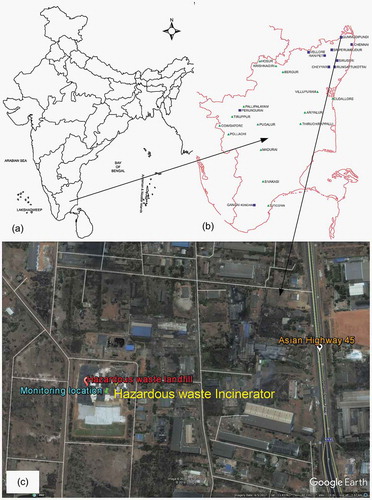
The measurement site (Gummidipoondi Town) is located 45 km north of Chennai City, Tamilnadu, with geographic position of 13.4069°N and 80.1103°E. Gummidipoondi is an industrial town in Chennai metropolitan region of Thiruvallur District of Tamil Nadu, India. It is bounded on the north by Andhra Pradesh State, on the east by the Bay of Bengal, on the south by Kanchipuram District, and on the west by Vellore District. The average annual rainfall for the location is 1104 mm, out of which 52% is received during northeast monsoon period (October–December) and the remaining 41% is received during southwest monsoon period (June–September). The study area location is shown in Figure 1. The study location lies on the thermal equator and is a coastal region, which prevents extreme variation in seasonal temperature. For most of the year, the weather is hot and humid. The highest temperature is recorded during the month of May. Solar irradiance is very intense on clear days, and depending upon the cloud cover the diffuse fraction varies. Temperature decreases from the middle of September. Since it is a coastal area, wind speed varies significantly across the year. During the study period, there was no rainfall recorded during the months of January to April. August and September recorded the maximum number of rainy days, and the maximum rainfall intensity was recorded during the month of December.

Figure 1. (a) Map of India. (b) Map of Tamil Nadu. (c) Map showing the study area at Gummidipoondi. (d) Aerial view of monitoring location. Image sources: Maps of India (a, b); Image Source: Google Earth Pro (c, d).

Methodology and data set

In this study, hourly measurements of air pollutants, namely, O₃, nitric oxide (NO), and nitrogen dioxide (NO₂), were carried out and in addition all the weather parameters have been measured from the weather station installed at the site. Study was conducted for the period from January 2016 to December 2016, and the data set monitored was used to study the characteristics during the study period.

Instrumentation

Emissions from industrial facilities, electric utilities, motor vehicle exhausts, etc., are some of the major sources of NO_x in the study area. Significant amounts of NO_x also originate from combustion of fossil fuels in power plants and industrial processes. The measurement of NO_x is being carried out by an nitrogen oxide analyzer, and the measurements are recorded continuously. An Environment S.A. Module 32M nitrogen oxide analyzer was used to measure the concentrations of NO, NO₂, and NO_x. The instrument principle is based on chemiluminescence technology. The minimum detectable limit of the instrument is about 0.4 ppb with automatic response time.

An Environment S.A. Module 42M O₃ analyzer was used to measure O₃ concentrations at the site. 42M is a continuous ozone analyzer. It uses the principle of ozone detection by absorption in ultraviolet light. The sample to the O₃ analyzer is taken through a Teflon tube connected to the back of the sampler unit. The ozone molecules selectively absorb the UV rays encountered on the 253.7 nm wavelength. The measurement cell holds the measurement detector as well as the reference detector and the UV lamp. A zero and span check is done once a week using the analyzer’s built-in ozone generator. The minimum detectable limit of the instrument is about 1 ppb with response time of 50 sec. Air is continually drawn via Teflon tube, by the analyzer’s internal pump. The analyzer continuously monitors the O₃ concentration and stores 2-min averages in a RAM data logger as well as 15-min averages at the end of this time period. The 15-min average is also displayed on the liquid crystal display (LCD) screen of the analyzer. Each hourly O₃ concentration is the average of four 15-min measurements taken during an hour and is reported as the hourly concentration.

The formation of ozone mainly depends on the precursor sources, whereas the dispersion of ozone depends on the meteorological parameters. Wind speed and wind direction play a significant role in the dispersion of ozone. Spectrum Watchdog 2000 series weather station model 2900ET together with Spec 9 pro software was used for monitoring the meteorological parameters at the site location. Meteorological parameters such as wind speed, wind direction, temperature, humidity, solar radiation, rainfall, and dew point can be measured with a minimum interval of 1 min. All the data were continuously monitored.

Data analysis

For analyzing the temporal characteristics, diurnal plots and seasonal plots were utilized. Diurnal plots and seasonal plots were made by using the average of hourly values of the chosen time period on 24-hr scale. Pearson’s correlation was used to understand the relationship between the different parameters. This was done using Statistical Package for Social Science (SPSS) version 22 (IBM, Armonk, NY). For studying the long-range transport, wind rose diagram, back-trajectory analysis, and retrievals from MOPITT (Measurement of Pollutants in the Troposphere) were used. MOPITT version 6 (Drummond, 1992) has been used to observe CO concentration. The data were available for the period between January 2016 and December 2016. The MOPITT instrument measures CO on board the Terra spacecraft, which is flying in polar sun synchronous orbit at an altitude of 705 km using upwelling infrared radiation near 4.7 μm (Deeter et al. 2009). The wind rose diagram was plotted using freeware WRPLOT View version 8.0.1. Back trajectories were calculated using Hybrid Single Particle Lagrangian Integrated Trajectory (HYSPLIT). Seven-day back trajectories arriving at the 10 m and 100 m surfaces were computed. Back-trajectory analysis ascertains the area of origin of air masses and determines source-receptor relationships.

Results and discussion

Temporal variation of surface-level ozone concentration

As per Indian Meteorological Department, each year is divided into four seasons: post-monsoon (January, February), summer (March–May), pre-monsoon (June–September), and monsoon (October–December). Table 1 shows the statistical summary of hourly O₃ concentration and other parameters measured during the study. The average wind speed was found to be highest in monsoon (4.99 m/sec) and lowest in post-monsoon (2.10 m/sec) seasons. Relative humidity varied from 29.72% to 100% during post-monsoon, 29.96% to 100% during summer, and 32.81% to 100% during pre-monsoon and monsoon seasons. Minimum relative humidity (RH) was recorded in summer season (29.96%). The daily average ambient temperature ranged from 19 to 34 °C during post-monsoon, 31 to 41 °C during summer, 25 to 41 °C during pre-monsoon, and 21 to 38 °C during monsoon seasons. The hourly average, maximum, and minimum concentrations for O₃ were found to be 17.74 ± 23.73, 497.232, and 1.11 μg/m³, respectively, during the study period. The hourly average NO₂ concentrations were in the range of 23.70 ± 8.76 μg/m³, with maximum and minimum daily average concentrations reaching up to 138.01 and 0.9 μg/m³, respectively. The hourly average, maximum, and minimum concentrations for NO were found to be 14.87 ± 4.09, 72.57, and 0.5 μg/m³, respectively. The concentrations of O₃, NO₂, and NO were found to be below the National Ambient Air Quality Standards (NAAQS India) during the study period. It was observed that 32% of the time in summer season, the hourly average O₃ concentrations were exceeding the NAAQS India value (180 μg/m³). The average concentration of O₃ in summer season was 29.66 ± 49.31 μg/m³, with maximum hourly concentration reaching up to 497.23 μg/m³ and minimum hourly concentration 4.32 μg/m³. Further, during monsoon season, the seasonal average, maximum, and minimum hourly O₃ concentrations were found to be 17.62 ± 19.84, 96.23, 2.81 μg/m³, respectively.

Table 1. Statistical summary of the attributes monitored during the study period.

Season	Attribute	Minimum	Maximum	Mean	Std. Dev
Summer	O3 (µg/m^3)	4.32	497.23	29.66	49.31
	RH (%)	29.96	100	69.31	14.55
	T(°C)	31	41	31.77	3.046
	W.D(degrees)	0	360	158.75	62.50
	W.S(m/s)	0	7.71	3.54	1.61
	NO(µg/m^3)	0.5	58.79	12.24	4.2
	NO2(µg/m^3)	0.9	96.41	20.47	5.7
Pre Monsoon	O3(µg/m^3)	1.11	292.36	21.38	25.77
	RH(%)	32.81	100	15.19	69.33
	T(°C)	25	41	31.77	3.05
	W.D(degrees)	0	350	74.25	193.75
	W.S(m/s)	0	7.76	3.53	1.65
	NO(µg/m^3)	1.5	82.19	16.39	6.78
	NO2(µg/m^3)	1.8	114.74	24.54	12.54
Monsoon	O3(µg/m^3)	2.1	96.23	17.62	19.84
	RH(%)	32.81	100	69.34	15.19
	T(°C)	21	38	30.22	2.99
	W.D(degrees)	0	346	193.75	74.75
	W.S(m/s)	0	10.28	4.99	1.43
	NO(µg/m^3)	1.1	66.2	17.94	8.2
	NO2(µg/m^3)	1.6	100.48	28.29	10.28
Post Monsoon	O3(µg/m^3)	2.63	144.13	27.39	29.64
	RH(%)	29.72	100	71.13	14.067
	T(°C)	19	34	3.15	26.70
	W.D(degrees)	0	360	77.25	68.25
	W.S(m/s)	0	7.2	2.10	1.74
	NO(µg/m^3)	2.1	72.57	14.7	14.2
	NO2(µg/m^3)	3.0	138.01	27.5	12.7

*W.D: Wind direction; W.S: Wind speed

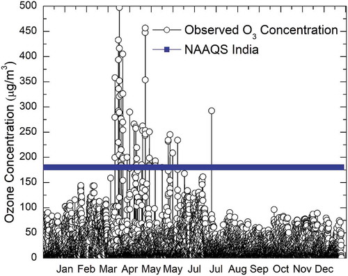
It can be observed from Figure 2 that there were many instances wherein the hourly ozone concentration exceeded the NAAQS standard of 180 µg/m³. O₃ values recorded at other seasons in India are reported in Table 2. A comparison of these values revealed that the O₃ values recorded in the present study are much higher than the values reported in other studies in India.

Table 2. Comparison of O₃ concentrations at different locations of India.

Study location	Site characteristic	Peak concentration (Season) (µg/m^3)	No. of Cases where in values exceeded NAAQS	Author and year
Gadanki	Rural	58 (Spring)	Nil	Naja and Lal 2002
Chennai	Industrial and Vehicular	135 (Summer)	Nil	Pulikesi et al. 2006
Pune	Industrial	104 (Winter)	Nil	Ali et al. 2012
Delhi	Vehicular and Industrial	152 (Post-monsoon)	Nil	Ali et al. 2012
Ooty	Clean zone	133 (Summer)	Nil	Udayasoorian et al. 2013
Mumbai	Vehicular	252 (Post-monsoon)	191 cases in 2 yr	Marathe and Murthy 2015
Gummidipoondi	Industrial and Vehicular	497.2 (Summer)	47 cases in 1 yr	Present study

Notes. Only the studies which have considered the data for the entire season are taken for comparison.

Figure 2. Time-series plot of hourly average O₃ concentrations.

Monthly variation of O₃ concentration during the study period is shown in Figure 3. It is evident from Figure 3 that the ozone concentrations were maximum during the two months of March and April and minimum concentrations occurred during the two months of September and December. The monthly variation of the daily 1-hr maximum, mean daytime (11 hr from 7:00 a.m. to 6:00 p.m.), and daily (24-hr) concentrations of O₃ during the study period are plotted in Figure 4. The highest monthly daytime (11 hr from 7:00 a.m. to 6:00 p.m.) and daily average O₃ concentrations were observed in summer season, especially March, with values around 58.88 μg/m³ (Figure 3). The daily concentration had another maximum in April with a value around 53.3 μg/m³. The lowest concentrations were observed in the month of September, with values as low as 19.66 and 27.68 μg/m³ for the daily and daytime concentrations, respectively. Prolonged duration of daytime, ample amount of solar radiation, and wind direction during the months of March and April resulted in thermal convections in these regions leading to higher mixing concentrations of ozone. From August to December, the conditions were reversed, with atmospheric temperature getting lower and there was record rainfall. Also, the presence of a stable atmosphere and shallowness of the atmospheric boundary layer led to a lower level of ozone. The temperature further decreased from December onward, and the wind speed increased. The prevailing winds flushed up particles to be lofted and dispersed spatially.

Figure 3. Monthly variation of ground level O₃ concentration during the study period.

Figure 4. Monthly variation of the daily 1-hr maximum, mean daytime (11 hr from 7:00 a.m. to 6:00 p.m.), and daily (24-hr) concentrations of O_3.

The diurnal variation of O₃, NO, and NO₂ is shown in Figure 5. From Figure 5, it can be seen that the O₃ concentration peaked during the noon and minimum concentration occurred during the early morning hours and during the nighttime. The O₃ variation during the study period was found to be unimodal. There were two peaks each for NO and NO₂, which corresponds to traffic (mostly truck loads) and some industrial emissions. The diurnal variation of ozone depends on many factors, such as altitude, solar zenith angle, advection potential, temperature, and the concentrations of halogens such as chlorine oxides (ClO_x). It can be observed that the pattern of ozone concentration followed the trend of solar radiation, with little modulation due to precursor emissions and meteorological conditions. This might be due to the fact that excessive temperature and solar irradiance promote the photochemical reaction, leading to high ozone concentration. In general, the warm periods are favorable to ozone photochemical reactions. The maximum concentration could also be composed of contribution from the precursors and the ozone that was transported from other polluted areas. The minimum concentrations typically occurred during the nighttime and early morning time. The photochemical processing of O₃ was halted due to the absence of the photochemical reactions. O₃ that stayed in the atmosphere was then consumed by deposition and/or reaction with NO, which acts as a sink for O₃ (Khoder 2007).

Figure 5. Diurnal variation of NO, NO₂, and O_3.

Effect of coastal wind on ozone formation and transportation

The wind rose diagrams of the site of measurement during different seasons are shown in Figure 6. The pattern of wind speed and wind direction was recorded throughout the study period. Unique pattern of sea breeze was observed during few days of the study period. Similar kind of phenomenon was reported by Adame et al. (2010) in the coastal area of southwestern Europe. During 4:00 a.m. to 8:00 a.m., the wind was blowing in the northeast direction and the wind speed ranged between 0.75 and 1.25 mph. Figure 7 shows the effect of wind on O₃ formation, and it can be observed that during midday, i.e., from 11:00 a.m. to 4:00 p.m., the wind direction was southeasterly (from the sea side), which is perpendicular to the coast line. The mean hourly wind speed varied between 2.25 and 3.75 mph. The ozone concentrations were found to be high on those time periods during particular days. This may be due to the fact that the sea breeze can transport the pollutants from the industrial area of Manali Town. Manali Town is classified as the critically polluted area by Central Pollution Control Board, India. The ozone transported from Manali Town also added to the maximum concentration of ozone observed during summer season. When the sea breeze stopped around 7:00 p.m., the wind speed went down to 0.3 mph. This observation is in accordance with the results reported by Pulikesi et al. (2006).

Figure 6. Wind rose plots during different seasons.

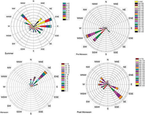
Figure 7. Peculiar pattern of wind speed and wind direction.

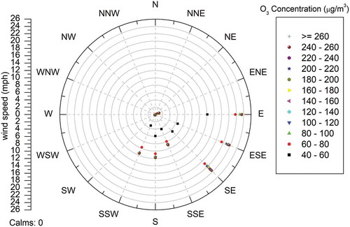
The relationship between O₃ concentration and wind direction is clearly depicted in Figure 8. Higher concentrations of O₃ were observed for the winds blowing from E, ESE, SE, SSE, and S relative to the onshore flow. This may be attributed to the chlorine (Cl) radical emitted from salt particles of the sea; it oxidizes VOCs at nearly double the level it does the hydroxyl radical (OH), which promotes the ozone formation at the coastline (Knipping and Dabdub 2003).

Figure 8. Scattered polar plot showing O₃ concentrations greater than 40 μg/m³ (circles represent the observed O₃ concentration).

Correlation and regression analyses of O₃ with temperature, solar irradiance, relative humidity, and NO_x concentration

The entire data set of hourly average O₃ concentration was clustered into four seasons and was used for correlation and regression analyses. Pearson’s correlation analysis was done for all the seasons, and the results are shown in Tables 3–6. In each season, the percentage of missing values was less than 2%. The missing values were eliminated from the analysis, as the formation of ozone is complex and nonlinear. Significant positive correlations were found between O₃, temperature, and solar irradiance. The correlations remained strong except during the monsoon months. The correlation between O₃ and RH was found to be NO_x dependent. NO_x concentration showed negative correlation with O₃, and the correlation was stronger and significant during all the seasons except the summer months. Also, during the nighttime, the correlation was stronger.

Table 3. Pearson’s correlation analysis of O₃ with temperature, solar irradiance, relative humidity, and NO_x during summer season (March, April, and May).

Pearson's r	T	SR	RH	NOx	O3
T	–	0.735	−0.930	0.075	0.561
SR	0.735	–	−0.789	−0.018	0.716
RH	−0.930	−0.789	–	−0.037	−0.567
NOx	0.075	−0.018	−0.037	–	0.247
O3	0.561	0.716	−0.567	0.247	–

*Correlation is significant at the 5% level.

Table 4. Pearson’s correlation analysis of O₃ with temperature, solar irradiance, relative humidity, and NO_x during pre-monsoon season (June, July, August, and September).

Pearson's r	T	SR	RH	NOx	O3
T	–	0.969	−0.976	−0.939	0.746
SR	0.969	–	−0.905	−0.833	0.751
RH	−0.976	−0.905	–	0.984	−0.656
NOx	−0.939	−0.833	0.984	–	−0.627
O3	0.746	0.751	−0.656	−0.627	–

*Correlation is significant at the 1% level.

Table 5. Pearson’s correlation analysis of O₃ with temperature, solar irradiance, relative humidity, and NO_x during monsoon season (October, November, and December).

Pearson's r	T	SR	RH	NOx	O3
T	–	0.433	0.491	0.035	−0.208
SR	0.433	–	0.002	−0.046	−0.122
RH	0.491	0.002	–	0.148	−0.265
NOx	0.035	−0.046	0.148	–	−0.533
O3	−0.208	−0.122	−0.265	−0.533	–

*Correlation is significant at the 5% level.

Table 6. Pearson’s correlation analysis of O₃ with temperature, solar irradiance, relative humidity, and NO_x during post-monsoon season (January and February).

Pearson's r	T	SR	RH	NOx	O3
T	–	0.768	−0.942	0.241	0.673
SR	0.768	–	−0.795	−0.135	0.775
RH	−0.942	−0.795	–	0.421	−0.668
NOx	0.241	−0.135	0.421	–	−0.519
O3	0.673	0.775	−0.668	−0.519	–

Notes. T = temperature; SR = solar Irradiance; RH = relative humidity; NO_x = nitrogen oxides.

The correlations of O₃ with its precursors are clearly depicted in Figure 9. It can be observed from (Figure 9a and b) that temperature and the solar irradiance are positively correlated with O₃. Nair et al. (2002) reported that the surface air temperature, which is a measure of solar insulation, leads to higher photochemical reaction. In monsoon months, comparatively low value of O₃ is attributed to low UV radiation intensities and low ambient temperatures. The values are highly significant at P < 0.01. Temperature acts as a surrogate of solar radiation, which in turn controls the photochemical reaction. This proves that both parameters have greater impact on O₃ formation. Season-wise analysis indicates that O₃ has stronger and positive correlations with temperature and solar irradiance during all the seasons except monsoon season. Although the rainfall was not observed during the daytime, the correlation is smaller and weaker. This may be due to a larger amount of O₃ transported from other locations rather than the ozone formation in situ.

Figure 9. Regression analysis. (a) O₃ with solar irradiance. (b) O₃ with temperature. (c) Negative correlation of O₃ with RH. (d) Positive correlation of O₃ with RH. (e) O₃ and NO_x during the summer months. (f) O₃ and NO_x during the monsoon months. (g) Plot showing background ozone.

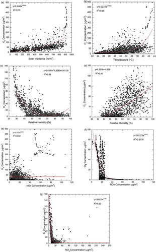
In the current study, both positive and negative correlations of O₃ with relative humidity were observed under different conditions. During the times when there is not much O₃ production at the site and the atmosphere is not substantially influenced by NO_x, negative correlation exists between O₃ and RH, as is shown in Figure 9c. The result is in concordance with the previous results reported in the literature (Ali et al. 2012; Khemani 1995). The reason for the above relationship is explained by Londhe et al. (2008): as the relative humidity increases, the major photochemical paths for removal of ozone are photolysis followed by the reaction of O_(1D) with water vapor and reaction of HO₂ with ozone (Londhe et al. 2008). Also, temperature and relative humidity are inversely correlated.

(1) ${\mathrm{O}}_3+\mathrm{h}\nu \to {\mathrm{O}}_2+{\mathrm{O}}_{(1\mathrm{D})}\lambda <310\mathrm{n}\mathrm{m}$(1)

(2) ${\mathrm{O}}_{(1\mathrm{D})}+{\mathrm{H}}_2\mathrm{O}\to 2\mathrm{O}\mathrm{H}$(2)

Furthermore, higher levels of humidity indicate that the cloud abundance is high, which in turn slows down the photochemical process.

On the contrary, positive correlation of O₃ occurs when the NO_x concentration is high and RH is greater than 80% (shown in Figure 9d) (Chen et al. 2019). The following reaction (eq 3) may happen under such conditions, resulting in the formation of O₃ molecules.

(3) $\left(\mathrm{N}{\mathrm{O}}_{\mathrm{X}}+\mathrm{O}\mathrm{H}+\right)\mathrm{V}\mathrm{O}\mathrm{C}+4{\mathrm{O}}_2+\mathrm{h}\nu \to 2{\mathrm{O}}_3+\mathrm{R}+{\mathrm{H}}_2\mathrm{O}\left(+\mathrm{N}{\mathrm{O}}_{\mathrm{X}}+\mathrm{O}\mathrm{H}\right)$(3)

When the values of NO_x are less than 80 μg/m³, NO_x is negatively correlated with O₃, as shown in Figure 9e. The correlation becomes positive when the values of NO_x are above 80 μg/m³. This may be due to faster photochemical dissociation and transport of NO_x at the same instant (Yang et al. 2019). The correlation between NO_x and O₃ is stronger during monsoon season and during the nighttime when the influence of solar irradiance and temperature is less, as illustrated in Figure 9f. During pre-monsoon and post-monsoon seasons, the correlation is not significant due to a sizeable number of points with elevated CO but low O₃, suggesting fresh pollution plumes that have not yet attained their O₃ production potential. Also, it can be observed that during monsoon and post-monsoon seasons, there is scattering of O₃ values, which indicates that there is another significant process apart from in situ O₃ formation. Figure 9g shows that even at zero NO_x levels, a significant amount of O₃ is observed in the study area and is termed as “background O₃.”

Long-range transport of pollutant air mass

It is evident from the regression plots that formation of ozone is mostly dependent on photochemistry, as the correlation is stronger and positive with solar irradiance and temperature. On the other hand, the correlation values are smaller; hence, apart from photochemistry, there could be some other mechanisms contributing to the observed O₃ concentration values. Also, there are records of only few days of rainfall that occurred during the nighttime.

It was also noted that there was slight variation in the seasonality across the year, unlike the northern part of the country wherein extreme temperatures used to be recorded. In spite of these conditions, the O₃ concentration decreased after the summer months.

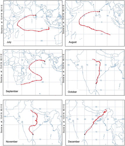
It has been reported in the literature (Mandal et al. 2015) that apart from formation in situ, transportation of pollutant air mass can further add to the concentration at a particular location. The likelihood of such occurrence was probed using National Oceanic and Atmospheric Administration (NOAA) Air Resources Laboratory’s Hybrid Single Particle Lagrangian Integrated (HYSPLIT) model, version 6 (http://www.arl.noaa.gov/ready.html). Mandal et al. (2015), Nair et al. (2002), and Sahu and Lal (2006) have reported that the advection of continental pollutants can modify the distribution of trace gases and titration reaction of pollutants. Seven-day backward trajectories for the study location are shown in Figure 10. It can be seen that during the months of October, November, December, and January, the air mass originates from the Indo-Gangetic Plain, whereas during the remaining months the air mass is from the Southeast Asian and marine (Indian Ocean) regions. This analysis is consistent with the analysis of Nair et al. (2011).

Figure 10. Monthly plots of 7-day isentropic backward-trajectory analysis using HYSPLIT4 trajectory model.

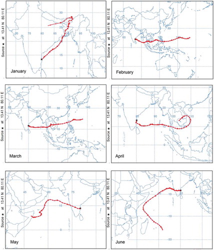
Figure 10. (Continued)

CO plays a major role in the formation of ground-level ozone and is used for the prediction of O₃ by many researchers (Abdul-Wahab et al., 2005; Özbay et al. 2011; Pavón-Domínguez, Jiménez-Hornero, and Gutiérrez de Ravé 2014; Rajab, MatJafri, and Lim 2013). The understanding of the correlation of O₃ with CO is at the stage of infancy. Few researchers have observed positive correlation of O₃ with CO (Abdul-Wahab et al., 2005; Özbay et al. 2011; Pavón-Domínguez, Jiménez-Hornero, and Gutiérrez de Ravé 2014) and vice versa (Rajab, MatJafri, and Lim 2013) . The distribution of CO is evident from Figure 11.

Figure 11. Monthly plot (Jan–Dec) of carbon monoxide at 900 hPa obtained from MOPITT.

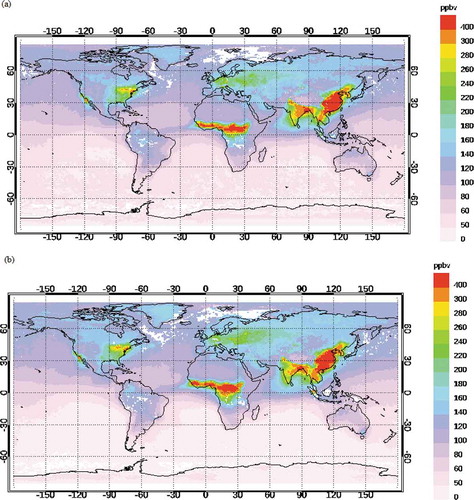
Figure 11. (Continued)

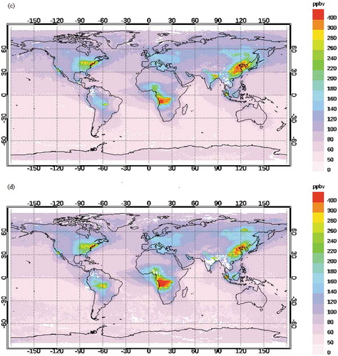
To explain the above continental transport of pollutant, monthly averaged spatial distribution of CO at 900 hPa obtained from MOPITT is plotted in Figure 11. The study site is very close to the Bay of Bengal region. Figure 11a shows that during January–February, a large plume of CO (>500 ppbv) is observed in the northeast Indian region and eastern region of China. In March, the intensity (strength as well as volume) of this plume (anthropogenic CO) has decreased (<400 ppbv) gradually when it intrudes into the Bay of Bengal region (Figure 11b). Hence, the continental transport has reduced during summer season. Due to the onset of southwest monsoon (June, July, August, and September), clean marine wind from the Southern Hemisphere has blown over the Bay of Bengal region (Figure 11c). Minimum concentration of O₃ is observed during this period. October onward, the concentration of anthropogenic CO has increased again over India and intrudes again into the Bay of Bengal region during the month of October only (Figure 11d). There is a steady upsurge of O₃ during the months of October, November, and December. The rainfall during this period dilutes the pollutant concentration. Similar features are noticed in the pattern of CO at 800 and 700 hPa.

Variation of O₃ concentration during weekends and weekdays

In the study location, lower NO_x levels and higher O₃ levels are observed during weekends and vice versa on weekdays. This is mainly due to the weekly changes in anthropogenic activities. In places where large weekday-weekend differences are present, the process of regional or local anthropogenic O₃ production dominates, whereas the areas dominated by the long-range transport present no weekend effect (Heuss, Kahlbaum, and Wolff 2003). Hence, the study of weekend effect in O₃ and NO_x levels can indicate appropriately the O₃ production. Weekdays were taken as from Monday to Friday, whereas Saturday and Sunday were considered weekend. In all four seasons, the daily average concentrations of O₃ and NO_x were noted, and the difference in their concentrations was calculated.

The reduction in traffic density and industrial operations during the weekends when compared with the weekdays was used to examine the relationship between O₃ and its precursors. Vehicular traffic and industrial emissions are the major sources of NO_x emission at the study site, where it is assumed that the weekend traffic density is lower than on weekdays. However, in spite of low weekend NO_x emissions, an elevated O₃ concentration was observed at the study site. Figures 12 and 13 show the diurnal variations of NO_x and O₃ concentrations on weekdays and weekends and the difference between weekends and weekdays (weekends minus weekdays) during the period of study. The O₃ concentration on weekends was greater than that on weekdays during all four seasons.

Figure 12. Diurnal variation of O₃ and NO_x during weekend and weekday.

Figure 13. Differences in weekend and weekday O₃ and NO_x concentrations

Fujita et al. (2003) placed the criteria used to identify the status of the weekend effect into three categories: (a) intense weekend effect if O₃ difference is >15 ppb; (b) moderate weekend effect if O₃ difference is 5–15 ppb; and (c) no weekend effect if O₃ difference is <5 ppb. Using the above criteria, intense weekend effect was noticed during summer season, whereas moderate weekend effect was observed in the other seasons. The mean hourly daytime differences between weekends and weekdays (weekends minus weekdays) ranged from 7 to 32.7 μg/m³ in summer, 3.8 to 14.5 μg/m³ in pre-monsoon, 4.6 to 9.2 μg/m³ in monsoon, and 0.1 to 4.5 μg/m³ in post-monsoon seasons (Figure 13). Meteorological conditions are also responsible to some extent for an intense weekend O₃ effect on a seasonal basis; however, it appears that differences in concentrations of O₃ precursors (NO_x and VOCs) are a major cause for the weekend O₃ effect in the study area.

Increased vehicular traffic density from Monday to Friday results in increased NO emission, which is responsible for decreased O₃ concentrations on weekdays compared with weekends due to the rapid reaction of NO with O₃. The reduction in NO emissions during the weekends results in the increased NO₂/NO_x ratio and consequently the titration reaction of O₃ by NO is reduced (Atkinson-Palombo, Miller, and Balling 2006). It also seems likely that ozone production efficiency is enhanced by the reduction in NO₂ and VOC levels, as these are major sinks for the key free radical species involved in conversion of NO to NO₂ without consumption of ozone. Lower NO levels and VOC emissions on weekend mornings consume less O₃, which accumulates later by photochemical reactions (Pudasainee et al. 2006), which may be more efficient in a lower-NO_x environment. Khoder (2009) also found many sites in Cairo with elevated O₃ on weekends when traffic and O₃ precursor levels were substantially reduced.

Furthermore, during the weekends, due to decreased traffic density, the concentration of fine particles decreases owing to the increase in solar radiation intensity. Hence, the photochemical formation dominates during the weekends (Marr and Harley 2002a, Marr and Harley 2002b). Researchers have observed that O₃ levels in the ambient air increased when emissions of NO_x decreased (Bernstein et al. 2004; Heuss, Kahlbaum, and Wolff 2003; Roberts-Semple, Song, and Gao 2012; Sadanaga et al. 2008).

Conclusion

Measurements of ground-level O₃ (hourly average) carried out in the industrial area of Chennai metropolitan region during January 2016 to December 2016 showed notorious peaks during the months of April, May, and June. The peak values recorded were about 1.5–2.8 times higher than that of NAAQS. Hazardous waste incineration produces large amounts of NO_x and CO, which might have resulted in the faster titration of O₃ during the night and early morning hours. Statistical analysis was carried out to ascertain the correlations between ground-level O₃ and NO_x and meteorological parameters. It was found that O₃ was positively correlated with temperature and solar irradiance and negatively correlated with relative humidity and NO_x.

The results of this study indicate that the ozone concentration in the study area exceeds the NAAQS standard during many days across the year. Therefore, O₃ control measures should be applied at least in the industrial areas in order to reduce the concentration of O₃. Furthermore, the reactivity of ozone with its precursors such as NO_x and VOCs has to be studied in order to develop the emission reduction policy for O₃ control. Also, for industrial sites, it would be better to formulate separate standards. This is because the workers are subjected to several kinds of pollutants and hence the standards have to be more stringent in order to safeguard the workers.

Acknowledgment

The authors gratefully acknowledge the NOAA Air Resources Laboratory (ARL) for granting the permission to use their HYSPLIT transport and dispersion model and/or READY Web site (http://www.arl.noaa.gov/ready.html) used in this publication. The authors would like to thank the anonymous reviewers for their useful suggestions, which helped in improving the quality of the paper.

Additional information

Funding

The authors thank the China Section of the Air & Waste Management Association for the generous scholarship they received to cover the cost of page charges and make the publication of this paper possible.

Notes on contributors

S. Mohan

S. Mohan is a professor in the Environmental and Water Resources Engineering Laboratory, Department of Civil Engineering, Indian Institute of Technology Madras, Chennai, India.

Packiam Saranya

Packiam Saranya is a Ph.D. scholar in the Environmental and Water Resources Engineering Laboratory, Department of Civil Engineering, Indian Institute of Technology Madras, Chennai, India.

References

- Abdul-Wahab, S. A., C. S. Bakheit, and S. M. Al-Alawi. 2005. Principal component and multiple regression analysis in modelling of ground-level ozone and factors affecting its concentrations. Environ. Model. Softw. 20:1263–71. doi:10.1016/j.envsoft.2004.09.001.
- Adame, J. A., E. Serrano, J. P. Bolívar, and B. A. de la Morena. 2010. On the tropospheric ozone variations in a coastal area of Southwestern Europe under a mesoscale circulation. J. Appl. Meteorol. Climatol. 49:748–59. doi:10.1175/2009JAMC2097.1.
- Ali, K., S. R. Inamdar, G. Beig, S. Ghude, and S. Peshin. 2012. Surface ozone scenario at Pune and Delhi during the decade of 1990s. J. Earth Syst. Sci. 121:373–83. doi:10.1007/s12040-012-0170-1.
- Atkinson-Palombo, C. M., J. A. Miller, and R. C. Balling Jr. 2006. Quantifying the ozone “weekend effect” at various locations in Phoenix, Arizona. Atmos. Environ. 40:7644–58. doi:10.1016/j.atmosenv.2006.05.023.
- Bernstein, J. A., N. Alexis, C. Barnes, I. L. Bernstein, J. A. Bernstein, A. Nel, D. Peden, D. Diaz- Sanchez, S. M. Tarlo, and P. B. Williams. 2004. Health effects of air pollution. J. Allergy Clin. Immunol. 114:1116–23. doi:10.1016/j.jaci.2004.08.030.
- Chen, Z., Y. Zhuang, X. Xie, D. Chen, N. Cheng, L. Yang, and L. Ruiyuan. 2019. Understanding long-term variations of meteorological influences on ground ozone concentrations in Beijing during 2006-2016. Environ. Pollut. 245:29–37. doi:10.1016/j.envpol.2018.10.117.
- CPCB. 2016. Guidelines for the Measurement of Ambient Air Pollutants (NAAQS). Cent. Pollut. Control Board, Gov. India.
- Deeter, M. N., D. P. Edwards, J. C. GIIIe, and J. R. Drummond. 2009. CO retrievals based on MOPITT near-infrared observations. J. Geophys. Res. Atmos. 114. doi:10.1029/2008JD010872.
- Drummond, J. R. 1992. Measurements of pollution in the troposphere (MOPITT). In The use of EOS for studies of atmospheric physics, eds. J. C. Gille and G. Visconti, 77–101. North Holland, Amsterdam.
- Finlayson-Pitts, B. J., and J. N. Pitts. 2000. Chemistry of the upper and lower atmosphere. Theory, experiments, and applications. 969. California: Academic Press. doi:10.1016/B978-0-12-257060-5.50027-7.
- Fujita, E. M., W. R. Stockwell, D. E. Campbell, R. E. Keislar, and D. R. Lawson. 2003. Evolution of the magnitude and spatial extent of the weekend ozone effect in California‘s South Coast Air Basin, 1981–2000. J. Air Waste Manage. Assoc. 53:802–15.
- Ghude, S. D., C. Jena, D. M. Chate, G. Beig, G. G. Pfister, R. Kumar, and V. Ramanathan. 2014. Reductions in India’s crop yield due to ozone. Geophys. Res. Lett. 41:5685–91. doi:10.1002/2014GL060930.
- Heuss, J. M., D. F. Kahlbaum, and G. T. Wolff. 2003. Weekday/weekend ozone differences: What can we learn from them? J. Air Waste Manage. Assoc. 53:772–88.
- Jacko, R., and T. La Breche. 2009. Air pollution and noise control. Environ. Eng. doi:10.1002/9780470432822.ch4.
- Jenkin, M. E., and K. C. Clemitshaw. 2002. Chapter 11 Ozone and other secondary photochemical pollutants: Chemical processes governing their formation in the planetary boundary layer. Dev. Environ. Sci. 1:285–338. doi:10.1016/S1474-8177(02)80014-6.
- Khemani, L. 1995. Study of surface ozone behaviour at urban and forested sites in India. Atmos. Environ. 29 (16):2021–24.
- Khoder, M. I. 2007. Ambient levels of volatile organic compounds in the atmosphere of Greater Cairo. Atmos. Environ. 41:554–66. doi:10.1016/j.atmosenv.2006.08.051.
- Khoder, M. I. 2009. Diurnal, seasonal and weekdays-weekends variations of ground level ozone concentrations in an urban area in greater Cairo. Environ. Monit. Assess. 149 (1–4):349–62.
- Knipping, E. M., and D. Dabdub. 2003. Impact of chlorine emissions from sea-salt aerosol on coastal urban ozone. Environ. Sci. Technol. 37:275–84. doi:10.1021/es025793z.
- Logan, J. A., M. J. Prather, S. C. Wofsy, and M. B. McElroy. 1981. Tropospheric chemistry: A global perspective. J. Geophys. Res. 86:7210. doi:10.1029/JC086iC08p07210.
- Londhe, A. L., D. B. Jadhav, P. S. Buchunde, and M. J. Kartha. 2008. Surface ozone variability in the urban and nearby rural locations of tropical India. Curr. Sci. 95 (12):1724–29.
- Mandal, T. K., S. K. Peshin, C. Sharma, P. K. Gupta, R. Raj, and S. K. Sharma. 2015. Study of surface ozone at Port Blair, India, a remote marine station in the Bay of Bengal. J. Atmos. Solar-Terrestrial Phys. 129:142–52. doi:10.1016/j.jastp.2015.04.010.
- Marathe, S., and S. Murthy. 2015. Seasonal variation in surface ozone concentrations, meteorology and primary pollutants in coastal mega city of Mumbai, India. J. Climatol. Weather Forecast. 3. doi:10.4172/2332-2594.1000149.
- Marr, L. C., and R. A. Harley. 2002a. Modelling the effect of weekday weekend differences in motor vehicle emissions on photochemical pollution in Central California. Environ. Sci. Technol. 36:4099–106. doi:10.1021/es020629x.
- Marr, L. C., and R. A. Harley. 2002b. Spectral analysis of weekday weekend differences in ambient ozone, nitrogen oxide and non-methane hydrocarbon time series in California. Atmos. Environ. 36:2327–35. doi:10.1016/S1352-2310(02)00188-7.
- Nair, P. R., D. Chand, S. Lal, K. S. Modh, M. Naja, K. Parameswaran, S. Ravindran, and S. Venkataramani. 2002. Temporal variations in surface ozone at Thumba (8.6°N, 77°E)-a tropical coastal site in India. Atmos. Environ. 36:603–10. doi:10.1016/S1352-2310(01)00527-1.
- Nair, P. R., L. M. David, I. A. Girach, and K. Susan George. 2011. Ozone in the marine boundary layer of Bay of Bengal during post-winter period: Spatial pattern and role of meteorology. Atmos. Environ. 45:4671–81. doi:10.1016/j.atmosenv.2011.05.040.
- Naja, M., and S. Lal. 2002. Surface ozone and precursor gases at Gadanki (13.5°N, 79.2°E), a tropical rural site in India. J. Geophys. Res. Atmos. 107. doi:10.1029/2001JD000357.
- Özbay, B., G. A. Keskin, Ş. Ç. Doǧruparmak, and S. Ayberk. 2011. Multivariate methods for ground-level ozone modeling. Atmos. Res. 102:57–65. doi:10.1016/j.atmosres.2011.06.005.
- Pandey, P., V. Irulappan, M. V. Bagavathiannan, and M. Senthil-Kumar. 2017. Impact of combined abiotic and biotic stresses on plant growth and avenues for crop improvement by exploiting physio-morphological traits. Front. Plant Sci. 8. doi:10.3389/fpls.2017.00537.
- Pavón-Domínguez, P., F. J. Jiménez-Hornero, and E. Gutiérrez de Ravé. 2014. Proposal for estimating ground-level ozone concentrations at urban areas based on multivariate statistical methods. Atmos. Environ. 90:59–70. doi:10.1016/j.atmosenv.2014.03.032.
- Pudasainee, D., B. Sapkota, M. L. Shrestha, A. Kaga, A. Kondo, and Y. Inoue. 2006. Ground level ozone concentrations and its association with NOx and meteorological parameters in Kathmandu valley, Nepal. Atmos. Environ. 40:8081–87. doi:10.1016/j.atmosenv.2006.07.011.
- Pulikesi, M., P. Baskaralingam, V. N. Rayudu, D. Elango, V. Ramamurthi, and S. Sivanesan. 2006. Surface ozone measurements at urban coastal site Chennai, in India. J. Hazard. Mater. 137:1554–59. doi:10.1016/j.jhazmat.2006.04.040.
- Rajab, J. M., M. Z. MatJafri, and H. S. Lim. 2013. Combining multiple regression and principal component analysis for accurate predictions for column ozone in Peninsular Malaysia. Atmos. Environ. 71:36–43. doi:10.1016/j.atmosenv.2013.01.019.
- Roberts-Semple, D., F. Song, and Y. Gao. 2012. Seasonal characteristics of ambient nitrogen oxides and ground-level ozone in metropolitan northeastern New Jersey. Atmos. Pollut. Res. 3:247–57. doi:10.5094/APR.2012.027.
- Sadanaga, Y., S. Shibata, M. Hamana, N. Takenaka, and H. Bandow. 2008. Weekday/weekend difference of ozone and its precursors in urban areas of Japan, focusing on nitrogen oxides and hydrocarbons. Atmos. Environ. 42:4708–23. doi:10.1016/j.atmosenv.2008.01.036.
- Sahu, L. K., and S. Lal. 2006. Distributions of C2-C5 NMHCs and related trace gases at a tropical urban site in India. Atmos. Environ. 40:880–91. doi:10.1016/j.atmosenv.2005.10.021.
- Thompson, A. M. 1992. The oxidizing capacity of the earth’s atmosphere: probable past and future changes. Science. 256:1157–65. doi:10.1126/science.256.5060.1157.
- Udayasoorian, C., R. M. Jayabalakrishnan, A. R. Suguna, S. Venkataramani, and S. Lal. 2013. Diurnal and seasonal characteristics of ozone and NOx over a high altitude Western Ghats location in Southern India. Adv. Appl. Sci. Res. 4:309–20.
- Vinikoor-Imler, L. C., E. O. Owens, J. L. Nichols, M. Ross, J. S. Brown, and J. D. Sacks. 2014. Evaluating potential response-modifying factors for associations between ozone and health outcomes: A weight-of-evidence approach. Environ. Health Perspect. doi:10.1289/ehp.1307541.
- Wang, W. C., X. Z. Liang, M. P. Dudek, D. Pollard, and S. L. Thompson. 1995. Atmospheric ozone as a climate gas. Atmos. Res. 37:247–56. doi:10.1016/0169-8095(94)00080-W.
- Yang, Y., X. Liu, J. Zheng, Q. Tan, M. Feng, Q. Yu, A. Junling, and N. Cheng. 2019. Characteristics of one-year observation of VOCs, NOX, and O3 at an urban site in Wuhan, China. J. Environ. Sci. 79:297–310. doi:10.1016/j.jes.2018.12.002.