Contribution of bioaerosols to airborne particulate matter

ABSTRACT

Fine and coarse particulate matter (PM), as measured, for example, in regulatory air pollution monitoring networks, contains biological entities such as fungal spores, pollen, animal dander, leaf wax, and human skin cells, to mention but a few types. Although these bioaerosols come in a wide range of particle size, of 14 common types nine fall into the 0– 10 µm range and four are in the 0– 2.5 µm range. These bioaerosols contribute to the concentrations of particulates determined by both filter-based and continuous instruments. This paper reviews bioaerosol research conducted worldwide in the last twenty years. Such studies have been conducted in Toronto, Canada, central Germany, Phoenix, Arizona, Davis, California, Dallas, Texas, and at many other sites worldwide. Notwithstanding the wide variety of climates, ecological systems, and urban and rural environments in which these measurements have been made, a reasonable, first-order estimate of the overall bioaerosol contribution to particles 2.5 microns and smaller (PM_2.5) is 16.5% and to particles 10 microns and smaller (PM₁₀) is 16.3%. A percentage contribution of this magnitude from unregulated emissions means that achieving PM standards will require greater reductions in the better understood anthropogenic and natural emissions of geological and combustion particles. In one such case the emission reductions necessary to achieve the standard increase from 25% (with bioaerosols ignored) to 36% (with bioaerosols accounted for). Although to the uninitiated this difference may not appear to be substantial, it can only be considered vast and nearly regulatorily impossible to those policy makers and regulators responsible for enacting emission-reduction regulations. Emissions of airborne biological materials are unregulated. Ignoring this natural component in attempting to achieve national ambient air quality standards for particulates can lead to overly optimistic predictions of attainment.

Implications: For those officials still striving to meet federal air quality standards for particulate matter, either PM₁₀ or PM_2.5, it would be prudent to acknowledge the presence of unregulated bioaerosols. Ignoring this portion of PM may lead to over-optimistic projections of attainment.

Introduction

Trends of emissions and concentrations of airborne fine particulate elemental and organic carbon in Phoenix, Arizona have been examined (Hyde 2013). This emissions research encompassed the urbanized portion of Maricopa County, Arizona (with Phoenix being the largest city in a metropolitan area of four million people). The research into the concentrations was limited to a single air pollution monitoring site called the James L. Guyton (JLG) Phoenix Supersite in central Phoenix. Operated by the Air Quality Division of the Arizona Department of Environmental Quality, this monitoring site also includes an array of samplers from the Interagency Monitoring of Protected Visual Environments (IMPROVE 2018) program, whose speciated fine particulate concentrations were used in the trends analysis. Two questions provoked by this research into carbonaceous particulates are: (1) How much of the measured particulate organic carbon can be attributed to bioaerosols? and (2) How much of airborne particulates in general can be attributed to bioaerosols? The second question is examined in this paper.

To express this question in regulatory language, how much do bioaerosols contribute to concentrations of fine particulate matter (PM_2.5) and to concentrations of particles 10 microns and smaller (PM₁₀)? As reviewed by ACGIH (1999), Monn (2002), McDermott (2004), Jaenicke, Matthias-Maser, and Gruber (2007), EPA (2008), Després et al. (2012), and Frohlich-Nowoisky et al. (2016), bioaerosols consist of proteins, lipids, carbohydrates (starch, cellulose), endotoxins, lipopolysaccharides, DNA, and RNA – originating in biological entities such as grass, shrubs, flowers, and trees (leaf wax, leaf litter, & pollen); fungi (fungal spores); humans (skin cells); dogs and cats (dander); bacteria; and viruses. Conventional knowledge places most of these organic particles in size ranges far larger than 2.5 microns; and, in their original, natural state, some, but by no means all, of these particles exceed 10 microns. But for at least one class of bioaerosols, the familiar pollen from grasses, shrubs, and trees, fragmentation takes place that produces biological particles well within this smaller size range. For example, grass pollens have been detected in fine particles, presumably from osmotic rupturing after lawn watering, leading to the release of starch granules in the size range of 0.6–2.5 microns (Knox and Suphioglu 1996). Pollen from shrubs and trees may be susceptible to similar rupturing after rainfall. Table 1 presents particle sizes for some of these bioaerosols.

Table 1. Particle sizes of bioaerosols (microns).

Bioaerosol	Particle size (microns)
Bacteria	1 − 5
Bacterial endotoxins	< 5
Fungi: ascospores and basidospores	2– 10
Amebae: Naegleria spp	10– 35
Amebae: Acanthamoeba spp	15– 45
Amebae: cysts of Acanthamoeba	10– 25
Amebae: cysts of Naegleria	7– 15
Viruses	0.02– 0.3
Dust mites: organisms	225– 520
Dust mites: fecal pellets	10– 35
Pollen: green microalgae (Chlorela vulgaris)	8– 10
Pollen: common names: carelessweed, dioecious amaranth, Palmer’s amaranth, Palmer amaranth, and Palmer’s pigweed (Amaranthus palmeri)	6
Pollen: Timothy grass (Phleum pretense)	22
Pollen: rye grass (Lolium arundinaceum)	40
Pollen: pine (Pinus, 126+ species)	50

Sources: ACGIH 1999; Sporomex 2018

Discussion #1: how much do bioaerosols contribute to particulates?

Bioaerosol monitoring and analysis conducted world-wide in the last 30 years provide enough empirical information to make a first-order estimate of their contribution to anthropogenic particulates. These anthropogenic particles come mostly from combustion or from mineral dusts disturbed and suspended by the mechanical action of machines, of vehicles and of gusty winds (Colls 2002). To a lesser but measureable degree, organic carbon particles also stem from secondary atmospheric chemical reactions of gaseous hydrocarbon emissions (Seinfeld and Pandis 1998). Complicating, if not compromising, any estimate of the bioaerosol contribution to airborne particulates, is the diverse set of climatic regimes sampled in this research. As measurement techniques for bioaerosols are delicate and expensive, the research community has simply been unable to quantify all the important bioaeresols at a single “representative” site for a long period of time. This lack of comprehensiveness for bioaerosols does not apply to the much less expensive and more easily accomplished environmental monitoring of common air pollutants and meteorological variables. Urban and rural ecosystems vary widely in their landscapes and climates, ensuring that no single site, even if extensively sampled, could be expected to have similar emission patterns and magnitudes of these biological particles. Nonetheless, the objective of this review is to apply these bioaerpsol measurements to the particular arid climate and urban micro-climate prevailing at one central Phoenix air monitoring site Despite the uncertainty engendered by the studies in their diverse climates and ecosystems, the utility of this approach lies in its communication to air pollution regulators and scientists. Most of these staff lack advanced biological training and experience and would not be expected to even be aware of the biological component of measured particulates. This review is an attempt to close that gap. In sum, even though only two such studies were conducted in metropolitan Phoenix (Boreson, Dillner, and Peccia 2004; Jia, Clements, and Fraser 2010), we conclude that bioaerosols contribute about 16 percent of the fine particulate matter (PM_2.5) in central Phoenix (bottom line of Table 2 and Figures 1 and 2). Likewise, a literature review of the bioaerosol contribution to PM₁₀ yields a somewhat lower percentage contribution – about 12%, as shown in Table 3.

Table 2. Bioaerosols in PM_2.5.

	Field work			Samples
Type	Location	Details	Season	duration (hours)	n	% of PM2.5	Reference
fungal spores and sub-pollen	2 urban sites, 1 rural site Toronto, Canada	Central, 50 m from busy roadway; NW suburban, commercial; rural, 100 km NNW	May, June	22h, n = several		4–11	Womilogu et al. (2003)
proteins	Hohenpeiss-enberg, Germany	On hill 300m above an agricultural area	May	24h n = 15		2.9 ± 1.1	Hock et al. (2008)
proteins	Phoenix, AZ 2 sites	Natural desert: Lost Dutchman State Park; Urban fringe of Phoenix (the suburb of Chandler)	winter spring summer	24h, n = 15, 5 each season		6.3 urban fringe; 19.0, desert	Boreson et al.(2004)
amino acids	Davis, CA	National Acid Deposition Program site, 2 miles SW of city center	annual	24h n = 9		3.3	Zhang and Anastasio (2003)
seven sugars	Jeju Island, w. North Pacific Ocean	Rural, cliff-side site	annual	24h n = 47		0.7*	Fu et al. (2012)
six sugars	Dallas, TX suburban Phoenix, AZ	Urban core (Dallas) Agricultural, suburban (Phoenix)	Jan – July Jan – April	24h n = 57 n = 45		0.6 0.5	Jia, Clements, and Fraser (2010)
arabitol mannitol	17 studies, world wide	Many and varied	?	?		0.15*	Bauer et al. (2008) Zhang and Anastasio (2003)
leaf litter	Los Angeles, CA	Los Angeles	annual	?		0.4*	Rogge et al. (1993) Rogge et al. (1996)
DNA	Germany	Munich, Hohenpeissenberg, & Zugspitze	?	4h n = 14		0.05	Després et al. (2012)
bacteria	?	?	?	?		0.0
Total						16.5**

*reported, not in percentages, but in gravimetric units (ng/m³), then converted to percentages using the Phoenix Supersite 2001–2011 November-January average of 13.99 μg/m³ for PM_2.5

**sum of the following: fungal spores & subpollen, average of 4% and 11% – 7.5%; proteins, average of 2.9% and 6.3% – 4.6%; amino acids, 3.3%; sugars, average of 0.5% and 0.6%, plus 0.15% – 0.6%; leaf litter, 0.4%; and DNA, 0.05% – for a grand total of 16.5%

Table 3. Bioaerosols in PM_10.

	Concentration (ng/m3)
Type of bioaerosol	Additive*	deferred**
I. Seven sugars	100.5
II. Arabitol		44
Mannitol		71
III. Arabitol, worldwide	21
Mannitol, worldwide	23
IV. Proteins, Germany		350
V. Amino acids	302
VI. DNA	7
VII. Bacteria	1.94E-04
VIII. Water-soluble groups	1923
IX. Proteins, metro PHX		1950
X. Fungal spores,pollen	3000
XI. Proteins, avg. IV. & IX.	1150
Total	6,526.5	ng/m3
[PM10] cent. PHX	40	ug/m3
% bio in [PM10]	16.3	%

*additive: values in this column have been added together to produce the sum of 6,526.5 ng/m3

**deferred: values in this column have been omitted from the sum to avoid double counting.

Figure 1. PM_2.5 composition November – January, Phoenix supersite.

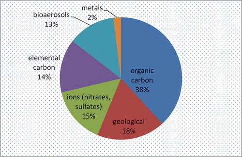
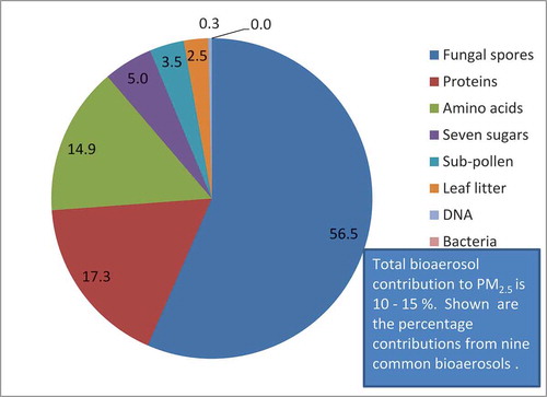
Figure 2. Distribution of bioaerosols in PM_2.5.

One aspect of these tables deserves a full explanation: namely, the expression of the bioaerosol “concentration” as a percentage of the long-term particulates concentrations at the central Phoenix monitoring site. The rationale for this is that the goal of the paper is to estimate how much of the measured particulates can be attributed to the biological components. For example, in Table 2, all of the bioaerosol measurements were reported in the literature as either gravimetric units or as colony forming units (the latter were converted to gravimetric units by using biological particle size and density), specific to the locale and timing of the sampling. Converting these concentrations to a percentage of the measured particulates is straightforward, but doing so brings up conflating a measurement in one location with its assumed prevalence in another. To take a single example, consider leaf litter, which was quantified in Los Angeles. What is the relation between leaf litter levels in the two urban areas? – a question that cannot be answered because the measurements have only been made in one place. The value of 0.4% comes from gravimetric (and analytical chemical) concentrations of leaf litter from Los Angeles, expressed in gravimetric units, and then converted to a percentage of the long-term particulates concentration in Phoenix. All the biological components have necessarily been so treated in these tables; it’s difficult to conceive of an alternative, given the extent of the information available.

Another point of explanation of Tables 2 and 3 might be helpful: i.e. the same bioaerosol measurement studies were relied on for both tables. The differences between Tables 2 and 3 are that in the former a long-term [PM_2.5] of 13.99 µg/m³ was employed and in the latter a comparable average concentration of [PM₁₀] of 40 µg/m³ was used. Table 3 also has two columns of concentrations in order to avoid double-counting concentrations from more than one study.

Discussion #2: relevance of bioaerosols in achieving PM standards

The bioaerosol component of airborne particulate matter poses its own health problems, whether viewed independently or in concert with the inorganic particles with which it is associated. Fungal spores, pollen, sub-pollen, bacteria, and viruses produce physiological stresses such as Valley fever, allergic reactions, asthma, and a multitude of diseases (ACGIH, 1999). When combined with particles emitted from anthropogenic activities such as transportation and nonroad heavy-duty vehicles and engines, these combinations of anthropogenic and natural particles enter the respiratory system and cause a variety of acute and/or chronic respiratory problems. Ambient air quality standards, in the U.S.A., Europe, and world-wide, have been developed and promulgated with the goal of protecting human health and environment (e.g. EPA 2019). In many countries in the developed world, and some in the developing as well, these standards have led to marked reductions in air pollutant emissions, to improved air quality, and to improved respiratory health. In areas whose pollutant concentrations exceed these standards, regulatory efforts on a local, regional, and national scale are undertaken to reduce emissions of pollutants and thereby achieve the standards.

Complications in achieving air quality standards, however, arise immediately when the precise nature of a measured air pollutant concentration is examined. Measured at a point in space, some 3– 10 meters above ground, ordinarily at an agency or private-sector fixed air monitoring site, this concentration actually comes about from a number of different but related emissions and transport phenomena. First, emissions in the immediate vicinity of the air pollution monitoring instrument lead to a portion of the measured concentrations. Second, emissions that take place a considerable distance from the monitor are transported to it by prevailing winds: these generalized urban emissions contribute another portion to the measured concentration (STI 2006). Third, continental and intercontinental transport of air pollutants has been observed, measured, and numerically modeled; these transported concentrations also contribute to the measured concentration. Fourth, even if there were no inter-regional transport, natural activities inside and outside urban areas lead to what are called “background” concentrations (WESTAR 2012). Decades of air monitoring and a multitude of special studies demonstrate that “zero” concentrations of pollutants cannot be found, even in remote hinterlands on continents or in remote islands. Fifth, regulatory efforts to reduce air pollutant emissions necessarily are directed towards the human activities that produce them; for example, cars that emit less pollution per mile driven. In the case of bioaerosols, however, which contribute to measured PM concentrations, this portion of the emitted aerosol largely escapes regulatory attention.

Consider the following arithmetic-based description of how much an urban area would need to reduce its air pollutant emissions to meet an air quality standard. As complicated as the spatial and temporal patterns of emissions can be, and as complex as the physical and chemical processes that govern the dispersal and atmospheric chemistry of the emitted pollutants, when considered at any physical scale of choice, air pollutant concentrations have to be roughly proportional to their emissions. Although reducing emissions lowers the concentrations of pollutants, the relationship is seldom linear. In the discussion below, brackets stand for concentrations of air pollutants and “PM” stands for airborne particulate matter.

${\left[\mathrm{P}\mathrm{M}\right]}_{\mathrm{m}}={\left[\mathrm{P}\mathrm{M}\right]}_{\mathrm{l},\mathrm{u},\mathrm{r}}+{\left[\mathrm{P}\mathrm{M}\right]}_{\mathrm{b}\mathrm{a}\mathrm{c}\mathrm{k}}+{\left[\mathrm{P}\mathrm{M}\right]}_{\mathrm{b}\mathrm{i}\mathrm{o},}\mathrm{w}\mathrm{h}\mathrm{e}\mathrm{r}\mathrm{e}$

[PM]_m is the measured PM concentration,

[PM]_l,u,r is that portion of the measured concentration that comes from local, urban, or regional emissions,

[PM]_back is the natural background concentration near the urban area in question,

[PM]_bio is the bioaerosol contribution.

Reducing local, urban, and regional emissions lowers the value of the first term but not the last two. If the air quality standard strived for is 150 µg/m³ (this value is the PM₁₀ 24-h standard in the U.S.A.) and [PM]_m is 200, then lowering the above-standard concentration to equal the standard can be done by subtracting 50, which is a (50/200) x 100% = 25% reduction. The emission reductions resulting in this lowered concentration, however, have no effect on either the background or bioaerosol contributions, which remain entirely unaffected by regulatory efforts. A representative value of background [PM₁₀] surrounding the Phoenix metropolitan area on an annual basis is 10 µg/m³; and on a 24-hour basis, under stagnant conditions leading to violations of the PM standard in the urban area, the value is about 30 µg/m³. These background estimates come from a long-term comparison of central Phoenix PM₁₀ concentrations with those measured at the Organ Pipe National Monument, a background site in the Sonoran Desert 180 miles south-southwest of Phoenix (Hyde 2003). Because bioaerosols contribute about 16.5% to [PM_2.5] and about 16.3% to [PM₁₀], a representative value for [PM]_bio on days leading to excessive PM concentrations would be 16.3% of 200, or 33 µg/m³. Under these constraints the arithmetic comes out as follows.

$\begin{array}{rl}& {\left[\mathrm{P}\mathrm{M}\right]}_{\mathrm{m}}={\left[\mathrm{P}\mathrm{M}\right]}_{\mathrm{l},\mathrm{u},\mathrm{r}}+{\left[\mathrm{P}\mathrm{M}\right]}_{\mathrm{b}\mathrm{a}\mathrm{c}\mathrm{k}}+{\left[\mathrm{P}\mathrm{M}\right]}_{\mathrm{b}\mathrm{i}\mathrm{o}}\\ & 200=137+30+33.\end{array}$

With the last two terms unchanged, then, the actual emission reduction to meet the standard has to be calculated from the first term, [PM]_l,u,r, which comes out to be (50/137) x 100% = 36%:

$\begin{array}{rl}& {\left[\mathrm{P}\mathrm{M}\right]}_{\mathrm{s}\mathrm{t}\mathrm{d}}={\left[\mathrm{P}\mathrm{M}\right]}_{\mathrm{l},\mathrm{u},\mathrm{r}}+{\left[\mathrm{P}\mathrm{M}\right]}_{\mathrm{b}\mathrm{a}\mathrm{c}\mathrm{k}}+{\left[\mathrm{P}\mathrm{M}\right]}_{\mathrm{b}\mathrm{i}\mathrm{o}}\\ & 150=87+30+33.\end{array}$

Although the difference in emission reductions needed to achieve the standard between not accounting and accounting for the background and bioaerosol contributions may appear slight – 25% vs. 36% – this margin becomes unmanageably large in the regulatory arena and may be partly responsible for the historical difficulty of Phoenix meeting the PM₁₀ standard.

One could argue that because the natural background already contains the bioaerosol portion, the latter component can be dropped. This assertion cannot be supported as stated, because if the background concentration is 16% bioaerosol, then [PM]_back could be set to 30 – (16% of 30) = 25 ug/m³, which would require a 40% reduction to meet the standard, an even wider gap above the theoretical 25%. Furthermore, the human, animal, and plant communities within the urban area that produce the emissions of bioaerosols are somewhat densely situated around the air monitoring site, relative to the natural countryside, in this case the Sonoran Desert. This urban plethora of bioaerosols – from fungi in the soil surface; from pollen and sub-pollen from lawns, flowers, shrubs, and trees; from leaf litter from plants; from skin, hair, and feather fragments from cats, dogs, humans, insects, and birds; and proteins and endotoxins from various biota – ensures a flux of bioaerosol emissions that necessarily contribute to the particulate concentrations as measured by regulatory air monitoring networks.

Conclusion

Fine particulates (PM_2.5) and particulates 10 microns and smaller (PM₁₀) are routinely measured in regulatory air pollution monitoring networks, have health standards set for them worldwide, degrade the respiratory health of the citizenry, and reduce the visibility of the airsheds. What may not be as obvious is that these particles contain materials emitted by biological organisms such as fungi, plants, and humans. To name but a few, these materials include human skin cells, pollen, DNA, RNA, proteins, sugars, and amino acids. These bioaerosols contribute to the gravimetric mass of particulates collected by filter-based and continuous air monitoring. Measurement programs conducted world-wide in the last 20 years have quantified these airborne biological particles: they can be expressed as percentages of total PM_2.5 or total PM₁₀. For example, as a percentage of PM_2.5, fungal spores and pollen contribute 8%; proteins, 3– 6%; amino acids, 3%; and various sugars, 0.2– 0.7%. A first-order estimate of the overall bioaerosol contribution to PM_2.5 is 16.5% and to PM₁₀ is 16.3%. These biological materials are unregulated. Not accounting for their contribution to PM in one case increases the percentage reduction of emissions necessary to meet the air quality standard from 25% to 36%. Ignoring them in crafting measures to achieve national ambient air quality standards for particulate matter leads inexoribly to overly optimistic predictions of attainment.

Additional information

Funding

This work has been partially supported by National Science Foundation (NSF) grant DMS 1419593 and U.S. Department of Agriculture (USDA) grant NIFA 2015-67003-23508.

Notes on contributors

Peter Hyde

Peter Hyde With a chemistry degree from the University of Illinois (Urbana), Mr. Hyde spent most of his 35 years in professional life in applied environmental science:  8 years in various positions with the Pima County Air Quality Control district (Tucson), 6 years investigating surface and ground water pollution for the Arizona Department of Environmental Quality, and 17 years pursuing air pollution science and regulation for the same agency.  Since retiring in 2007 he has conducted air pollution research at the Arizona State University’s Tempe campus. Recent projects, most in collaboration with other researchers, have been (1) PM₁₀ and childhood asthma in Phoenix, (2) community-wide risk assessment for air toxics for metropolitan Phoenix (for the Joint Air Toxics Assessment Project), (3) air toxics emissions inventory for the same project, (4) a similar risk assessment for the Yuma, AZ, San Luis, Rio Colorado, Sonora region, (5) trends in emissions and concentrations (2001 – 2011) of particulate elemental and organic carbon in central Phoenix, (6) the contribution of bioaerosols to airborne particulates, and (7) comparison of filter-based and continuous PM₁₀ measurements in Nogales, AZ.

Alex Mahalov

Alex Mahalov received a Ph.D. degree in applied mathematics from Cornell University in 1991. He held a post-doctoral position with the Department of Mechanical Engineering, UC Berkeley. He joined Arizona State University, where he was promoted to the Wilhoit Foundation Dean’s Distinguished Professor in 2008. He has authored over 150 research articles and scientific reports. Dr. Mahalov is currently developing next generation earth system models and data assimilation strategies with applications to food-energy-water systems. These models encompass the processes and interactions among agricultural meteorology, chemistry, hydrology and biophysics. Practical applications include integrated studies of air quality and development of mitigation strategies to reduce ozone and particulate matter concentrations to sustain healthy urban environments.

References

- ACGIH, American Conference of Governmental Industrial Hygienists. 1999. Bioaerosols: Assessment and control. ed. J. Macher, Cincinnati, OH: The American Conference of Governmental Industrial Hygienists.
- Bauer, H., M. Claeys, R. Vermeylen, E. Schueller, G. Weinke, A. Berger, and H. Puxbaum. 2008. Arabitol and mannitol as tracers for the quantification of airborne fungal spores. Atmos. Environ. 42:588–93. doi:10.1016/j.atmosenv.2007.10.013.
- Boreson, J., A. M. Dillner, and J. Peccia. 2004. Correlating bioaerosol load with PM2.5 and PM10 concentrations: A comparison between natural desert and urban-fringe aerosols. Atmos. Environ. 38:6029–41. doi:10.1016/j.atmosenv.2004.06.040.
- Colls, J. 2002. Air pollution. 2nd ed., 87–89. London: Spon Press.
- Després, V. R., J. A. Huffman, S. M. Burrows, C. Hoose, A. Safatov, G. Buryak, J. Fröhlich-Nowoisky, W. Elbert, M. Andreae, U. Pöschl, et al. 2012. Primary biological aerosol particles in the atmosphere: A review. Tellus B 64: 857–95.
- EPA. 2008. A review of the impacts of climate variabi lity and change on aeroallergens and their associated effects. EPA/600/R-06/164F. U.S. EPA.
- EPA. 2019. National ambient air quality standards. Accessed February, 2019. https://www.epa.gov/criteria-air-pollutants/naaqs-table.
- Frohlich-Nowoisky, J., C. J. Kampf, B. Weber, J. A. Huffman, C. Pöhlker, M. O. Andreae, N. Lang-Yona, S. M. Burrows, S. S. Gunthe, W. Elbert, et al. 2016. Bioaerosols in the Earth system: Climate, health, and ecosystem interactions. Atmos. Res. 182:346–76. doi:10.1016/j.atmosres.2016.07.018.
- Fu, P., K. Kawamura, M. Kobayashi, and B. R. T. Simoneit. 2012. Seasonal variations of sugars in atmospheric particulate matter from Gosan, Jeju Island: Significant contributions of airborne pollen and Asian dust in spring. Atmos. Environ. 55:234–39. doi:10.1016/j.atmosenv.2012.02.061.
- Hock, N., J. Schneider, S. Borrmann, A. Römpp, G. Moortgat, T. Franze, C. Schauer, U. Pöschl, C. Plass-Dülmer, and H. Berresheim. 2008. Rural continental aerosol properties and processes observed during the Hohenpeissenberg aerosol characterization experiment (HAZE2002). Atmos. Chem. Phys. 8:603–23. doi:10.5194/acp-8-603-2008.
- Hyde, P. 2003. Organ pipe dichotomous PM concentrations. unpublished (available from the author).
- Hyde, P. 2013. Trends in ambient concentrations of elemental and organic carbon in light of increasingly cleaner fuels and engines, 48pp. prepared for Arizona Department of Environmental Quality .unpublished (available from the author).
- IMPROVE. 2018. Interagency monitoring of protected visual environments. Accessed June, 2018. http://vista.cira.colostate.edu/IMPROVE/.
- Jaenicke, R., S. Matthias-Maser, and S. Gruber. 2007. Omnipresence of biological material in the atmosphere. Environ. Chem. 4:217–20. doi:10.1071/EN07021.
- Jia, Y., A. L. Clements, and M. P. Fraser. 2010. Saccharide composition in atmospheric particulate matter in the southwest US and estimates of source contributions. J. Aerosol Sci. 41:62–73. doi:10.1016/j.jaerosci.2009.08.005.
- Knox, B., and C. Suphioglu. 1996. Environmental and molecular biology of pollen allergens. Trends Plant Sci. 1:156–64. doi:10.1016/S1360-1385(96)80051-3.
- McDermott, H. 2004. Air monitoring for toxic exposures. 2nd ed., 473–503. Hoboken, NJ: John Wiley & Sons.
- Monn, C. 2002. Exposure assessment of air pollutants. In Air pollution science for the 21st century, ed. J. Austin, P. Brimblecombe, and W. Sturges, 148–51. Oxford, UK: Elsevier Science Ldt.
- Rogge, W., L. M. Hildemann, M. A. Mazurek, G. R. Cass, and B. R. T. Simoneit. 1993. Sources of fine organic aerosol. 4. particulate abrasion products from leaf surfaces of urban plants. Environ. Sci. Technol. 27:2700–13. doi:10.1021/es00049a008.
- Rogge, W., L. M. Hildemann, M. A. Mazurek, G. R. Cass, and B. R. T. Simoneit. 1996. Mathematical modeling of atmospheric fine particle-associated primary organic compound concentrations. J. Geophys. Res. 101 (no. D14):19,379–19,394, August 27. doi:10.1029/95JD02050.
- Seinfeld, J., and S. Pandis. 1998. Atmospheric chemistry and physics, 724–43. New York: John Wiley & Sons.
- Sporomex. 2018. Accessed December, 2018. http://www.sporomex.co.uk/technology/51-pollenspores.
- STI. 2006. Regional and local contributions to peak local ozone concentrations in six western cities. for WESTAR (Western States Air Resources Council; STI: Sonoma Technologies, Inc.
- WESTAR. 2012. Background ozone in the U.S. A conference on western ozone transport.
- Womilogu, T., et al. 2003. Methods to determine the biological composition of particulate matter collected from outdoor air. Atmos. Environ. 37:4335–44. doi:10.1016/S1352-2310(03)00577-6.
- Zhang, Q., and C. Anastasio. 2003. Free and combined amino compounds in atmospheric fine particles (PM2.5) and fog waters from Northern California. Atmos. Environ. 37:2247–58. doi:10.1016/S1352-2310(03)00127-4.