Reflecting on progress since the 2005 NARSTO emissions inventory report

ABSTRACT

Emission inventories are the foundation for cost-effective air quality management activities. In 2005, a report by the public/private partnership North American Research Strategy for Tropospheric Ozone (NARSTO) evaluated the strengths and weaknesses of North American emissions inventories and made recommendations for improving their effectiveness. This paper reviews the recommendation areas and briefly discusses what has been addressed, what remains unchanged, and new questions that have arisen. The findings reveal that all emissions inventory improvement areas identified by the 2005 NARSTO publication have been explored and implemented to some degree. The U.S. National Emissions Inventory has become more detailed and has incorporated new research into previously under-characterized sources such as fine particles and biomass burning. Additionally, it is now easier to access the emissions inventory and the documentation of the inventory via the internet. However, many emissions-related research needs exist, on topics such as emission estimation methods, speciation, scalable emission factor development, incorporation of new emission measurement techniques, estimation of uncertainty, top-down verification, and analysis of uncharacterized sources. A common theme throughout this retrospective summary is the need for increased coordination among stakeholders. Researchers and inventory developers must work together to ensure that planned emissions research and new findings can be used to update the emissions inventory. To continue to address emissions inventory challenges, industry, the scientific community, and government agencies need to continue to leverage resources and collaborate as often as possible. As evidenced by the progress noted, continued investment in and coordination of emissions inventory activities will provide dividends to air quality management programs across the country, continent, and world.

Implications: In 2005, a report by the public/private partnership North American Research Strategy for Tropospheric Ozone (NARSTO) evaluated the strengths and weaknesses of North American air pollution emissions inventories. This paper reviews the eight recommendation areas and briefly discusses what has been addressed, what remains unchanged, and new questions that have arisen. Although progress has been made, many opportunities exist for the scientific agencies, industry, and government agencies to leverage resources and collaborate to continue improving emissions inventories.

Introduction

Having a quantitative understanding of air pollutant emissions in North America is critical to public health in communities across Canada, the United States, and Mexico. An emissions inventory depends on a wide variety of information, including measurements from industry; submissions from state, local, and tribal partners; meteorological data; activity levels such as the number of miles driven by gasoline-fueled cars in a county; and other estimates based on the best available science. These inputs are incorporated into multiple emissions inventory models and undergo quality assurance checks and are reviewed by stakeholders. The resulting inventories are then used for emissions forecasting, near-term air quality forecasting, environmental and human health impact analyses, international reporting requirements, and regulatory air quality modeling and planning. With so many uses for emissions inventories, it is critical that they be used and maintained appropriately. Depending on the intended purpose, the use of an emissions inventory may change, which will affect the importance of specific characteristics of the inventory.

While emissions management and regulatory activities are well supported by current inventories, a key part of the inventory development process is to continually update them to reflect new discoveries, data sources, or changes in processes, infrastructure, and air quality standards. For example, since the 1970s, there have been steep declines in emissions from motor vehicles and power plants across most of the United States due to the successful implementation of controls for five key pollutants: carbon monoxide (CO), volatile organic compounds (VOCs), sulfur dioxide (SO₂), nitrogen oxides (NO_x), and particulate matter (PM) (U.S. EPA, 2018a). This accomplishment, coupled with changes in U.S. energy infrastructure, has led to a need to better quantify emissions from a variety of other sources that previously had less relative impact on total pollutant concentrations. In recent years, effective modern air quality planning has required knowledge and quantification of emissions from smaller and more distributed sources, as well as knowledge of additional chemical species. Over a decade ago, the greatest concern for transportation emissions was solid particulate and gaseous tailpipe emissions; improvements in technology have decreased tailpipe emissions and now the formation of secondary organic aerosols in the atmosphere has become an active area of research (Carlton et al. 2010). Another example is the extraction and processing of oil and gas occurring across much of the United States. A decade ago, this was a small contributor to most criteria emissions inventories, but oil and gas development has escalated rapidly in the past decade due to advances in technology that decreased the cost associated with extraction of these resources (U.S. EIA, 2018). These emissions are distributed over a substantial number of activities, which vary greatly across the lifetime of a well (e.g. drilling, extraction, decommissioning). Additionally, variability exists in controls, development and management practices, and composition across different locations and companies. This sector, among many others, offers opportunities for the incorporation of emerging methods and traditional technologies to improve emissions inventories.

To identify the strengths and weaknesses of North American emissions inventories, years of research were compiled in the 2005 publication “Improving Emission Inventories for Effective Air Quality Management Across North America: A NARSTO Assessment.” The North American Research Strategy for Tropospheric Ozone (NARSTO), a public/private partnership that worked towards improved air quality management in North America, convened a panel of experts to examine the state of emission inventories in the early 2000s for Canada, the United States, and Mexico (Miller et al. 2006; NARSTO 2006; Pennell and Mobley 2006). From this collaboration, emissions inventory needs were presented as eight key elements:

1. Reduce uncertainties associated with emissions from key under-characterized sources

2. Improve speciation estimates

3. Improve existing emissions inventory tools and develop new ones

4. Quantify and report uncertainty

5. Increase inventory compatibility and compar-ability

6. Improve user accessibility

7. Improve timeliness

8. Assess and improve emission projections

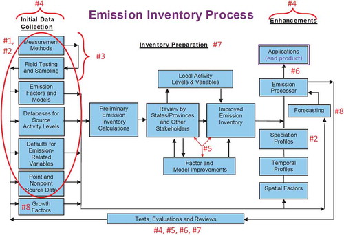
Significant progress has been made since the NARSTO assessment was published in 2005. This paper will review the eight recommendation areas and briefly discuss what has been addressed, what remains unchanged, and what new questions have arisen. Although the original NARSTO assessment covered North America, this review focuses on the United States (U.S.) National Emissions Inventory (NEI), with an emphasis on the 2014 NEI which is the most recent version available (U.S. EPA, 2018g, 2018h). Mexican and Canadian inventories will be briefly explored under Recommendation #5 below. Figure 1 is reproduced from the NARSTO assessment and represents a simplified emissions inventory development process. Red numbers have been added to indicate how each of the eight recommendations most closely corresponds to parts of this process.

Figure 1. Emissions inventory development flowchart, from Figure 2.1 of the 2005 NARSTO assessment, updated in red with the relevant recommendation sections corresponding to each part of the process.

Background on emissions inventories in the United States

The U.S. Environmental Protection Agency (EPA) compiles a comprehensive set of air emissions data every three years that includes five directly emitted criteria pollutants (particulate matter, carbon monoxide, sulfur oxides, nitrogen oxides, and lead), precursors of criteria pollutants (i.e. NO_x and VOCs for ozone and particulate matter, NH₃ and SO₂ for particulate matter alone), and hazardous air pollutants (HAPs). Greenhouse gases are also compiled for selected source sectors such as mobile sources, wildfires, and prescribed fires. The NEI provides emission values for particulate matter, carbon monoxide, sulfur oxides, nitrogen oxides, ammonia, and VOC pollutants on a county or sub county basis (depending on the source category) and is largely based on data provided by state, local, and tribal (SLT) agencies. These include, but are not limited to, county-level annual emissions, process-level emissions for major point sources, and day-specific fires. EPA provides emission estimates, methodology, guidance, and some tools to estimate emissions and reviews SLT agency submissions, filling in gaps when necessary. Emissions from onroad vehicles and nonroad engines are estimated in the newest NEIs (e.g. 2014) using the MOtor Vehicle Emissions Simulator (MOVES) (U.S. EPA, 2018b). Earlier NEI estimates used the older MOBILE6 or NONROAD model. Some states provide detailed MOVES inputs describing vehicle activity, populations, age distributions, and local control programs, while others rely on MOVES defaults and data EPA compiles from sources such as the Federal Highway Administration. Likewise, some states voluntarily report HAPs to the NEI; otherwise, this information is taken from the annual Toxic Release Inventory (TRI) for many point sources, which includes HAPs and other toxic chemicals that are reported by facilities to EPA (U.S. EPA, 2018c). The EPA uses available literature and additional tools to gap fill missing HAP data not supplied by the states and not found within the TRI. Additional emission factors are derived from the EPA AP-42 and WebFIRE programs (U.S. EPA, 2011, 2018d), which collect criteria and other pollutant emissions factors from a variety of industries and other source measurement research applications. Many EPA tools include complex models, such as EPA’s oil and gas tool, which are publicly available and under continual development by the Agency.

Greenhouse gas (GHG) information is also collected by the EPA separate from the NEI. This is a new addition to the emission inventory portfolio since the 2005 NARSTO assessment and is discussed as it relates to the goals of the original assessment. Large facilities, fossil fuel suppliers, industrial gas suppliers, and facilities that inject carbon dioxide greater than 25,000 metric tons of carbon dioxide equivalent (mtCO₂e) or more are required to report annual greenhouse gas emissions under the Greenhouse Gas Reporting Program (GHGRP) (U.S. EPA, 2018e). EPA also compiles the Inventory of U.S. Greenhouse Gas Emissions and Sinks (GHG Inventory) (U.S. EPA, 2018f), which includes all anthropogenic emissions and sinks at the national level as part of obligations to report inventories to the United Nations Framework Convention on Climate Change (UNFCCC, 2018). Both programs are managed and implemented on an annual reporting cycle and are focused on the national trend using the latest methods.

Emission inventories have a variety of uses, including providing input for pollution reduction strategies, calculating pollution trends over time, and providing input for chemical transport models and dispersion models. In addition to emissions inventories, an emissions modeling platform for the U.S. contains other data files, software tools, and scripts that process the emissions into the form needed for air quality modeling. This includes information necessary to disaggregate annual county-level emissions as reported in the NEI into hourly emissions on spatially resolved grids (often at resolutions of 36 km x 36 km, 12 km x 12 km, or 4 km x 4 km) for individual model mechanism chemical species. Each EPA-distributed emissions modeling platform supports air quality modeling of an historic year and sometimes includes projected inventories for one or more years into the future. Emissions modeling platforms are documented and publicly available at https://www.epa.gov/air-emissions-modeling. Other regulatory agencies and individual research groups may also have their own emission modeling platforms.

Findings

Each of the following sections identifies a set of findings and recommendations from the 2005 NARSTO report and then summarizes developments since the 2005 report.

Section 1: Reduce uncertainties associated with emissions from key under-characterized sources

• NARSTO Finding: Few source categories are well characterized and reported; many source categories are uncertain, especially non-point sources.

• NARSTO Recommendation: Focus immediate measurement and development efforts on areas of greatest known uncertainty, systematically apply sensitivity and uncertainty analyses to identify subsequent improvement priorities. The following pollutants and emissions sources were identified as the top 10 most uncertain:

  • Fine particles and their precursors

  • Toxic and hazardous air pollutants

  • Onroad motor vehicles

  • Agricultural sources, especially ammonia

  • Biogenic sources

  • Petrochemical industrial facilities

  • Off-road mobile sources

  • Open biomass burning

  • Residential wood combustion

  • Paved and unpaved road dust

Since the report, some of these source categories have received extensive attention and as a result are better characterized, while other under-characterized sectors remain uncertain.

EPA has invested in intramural and extramural research to improve the science of emission models and measurement methods used by the air quality management community. The EPA’s Science To Achieve Results (STAR) program has administered several sets of grants that have addressed sources of uncertainties identified in the NARSTO assessment (Appendix A). Research into fine particles (defined as particulate matter under 2.5 µm in diameter, or PM_2.5) from onroad motor vehicles, biogenic sources (naturally-emitted compounds like isoprene and terpenes), and open biomass burning (wildfires or other fires) have received significant investment (e.g. Wagstrom et al. 2014). While the primary purpose of STAR grants is to address knowledge gaps for the benefit of the broad scientific and air quality management community, EPA has worked to incorporate new knowledge from STAR projects and other research efforts in the community to improve the NEI process. For example, one STAR-funded project resulted in the development of a farm emissions model to predict ammonia emissions based on varying animal type, manure management practices, and meteorology (McQuilling and Adams 2015), which helped improve a more simplistic model used by the National Emissions Inventory at the time of the NARSTO report. This model was used to develop livestock waste ammonia emissions for the 2014 NEI.

Currently, EPA is collaborating with other states and regional offices in the development of the 2016 modeling platform, which incorporates the latest improvements in the 2014 NEI as well as subsequent improvements. Maintaining connections with extramural researchers is recommended for continued NEI improvements, especially for non-NEI year emission estimates. Independent researchers wishing to include their research in the NEI should be mindful of the variety of EPA collaborations (including STAR grants) that exist. For more information on the 2014 NEI, an interactive story map was developed by EPA that allows readers to see estimates for emissions via various tables and charts at https://gispub.epa.gov/neireport/2014/(U.S. EPA 2018g). It does not specifically address which improvements have occurred but could be used as a comparison to future NEIs.

Overall emissions research advances are highlighted below, grouped into three broad emissions sources: anthropogenic, natural, and fires.

Anthropogenic sources

Numerous improvements in methodologies and data for anthropogenic emissions have been implemented in response to many of the NARSTO recommendations and are documented in EPA’s modeling platform technical support document (Eyth and Vukovich 2016). In this section, we highlight some key areas of progress, but do not attempt to cover all sources as a comprehensive review of uncertainties from all anthropogenic emissions sources is beyond the scope of this paper. For any source category not covered here, the reader is encouraged to consult the technical support document associated with an emission modeling platform; for the 2011 platform, details can be found in Eyth and Vukovich (2016). In addition, a technical support document for the 2014 NEI version 2 is available which provides full technical details for the emissions inventory (U.S. EPA 2018h).

Inventories for cars, trucks and other onroad mobile sources have improved significantly in terms of information and detail. However, the impact of these changes on air quality models has yet to be confirmed independently in a peer-reviewed study. In 2010, EPA replaced the MOBILE6 model with the Motor Vehicle Emission Simulator (MOVES), a state-of-the-art upgrade to EPA’s modeling tools for estimating emissions from highway vehicles, based on analysis of millions of emission test results and considerable advances in the Agency’s understanding of vehicle emissions (U.S. EPA, 2013). Further details on the data and emission testing used in development of the MOVES model can be found in the MOVES Onroad Technical Reports library (U.S. EPA, 2018i). The model has been substantially updated, and as of February 2019, the current version is MOVES2014b. The MOVES generation of models is not merely an upgrade of the previous MOBILE model using more recent emissions data; it is brand-new software, designed from the ground up to estimate emissions at a more detailed level. The more detailed approach to modeling allows EPA to easily incorporate large amounts of data from a wide variety of sources, such as data from vehicle inspection and maintenance programs, remote sensing devices certification testing, and portable emission measurement systems. Improvements include:

• A detailed analysis of 70,000 vehicles in Arizona’s vehicle inspection and maintenance program provides information on how emissions from vehicles from the late-1990’s and early 2000’s change with age (U.S. EPA, 2015; Warila 2009).

• Other inspection & maintenance, remote sensing, and special purpose studies helped EPA to better understand trends in VOC, CO, and NO_x emissions for light-duty cars and trucks (U.S. EPA 2018i).

• A landmark study of PM emissions, testing nearly 500 gasoline-fueled light-duty cars and trucks in Kansas City, Missouri, was undertaken by a collaborative effort including EPA, the Department of Transportation, the Department of Energy, and the automotive and petroleum industries (Fulper et al. 2010; U.S. EPA, 2008a, 2008b). The Kansas City study confirmed that PM emissions from light-duty gasoline-fueled vehicles were higher than previously predicted and showed that cold ambient temperatures can dramatically increase PM start emissions (Nam et al. 2010). Increases in PM start emissions at low temperatures are now included in MOVES.

• More than 400 in-use trucks were tested, some in the laboratory and some with on-road measurement equipment, to show how real trucks pollute at a range of speeds and driving conditions (U.S. EPA, 2012). EPA also better incorporated emissions from heavy-duty diesel crankcase ventilation and from extended idling (also known as “hotelling”) – two emission processes that were relatively unstudied at the time of the NARSTO report (U.S. EPA 2012). The incorporation of these additional data led to increases in heavy-duty NO_x and PM emissions from MOVES.

• The MOVES model incorporates the modeling of new regulations including the Tier 3 emission standards, which begin to phase in 2017 for cars, light-duty trucks, medium-duty passenger vehicles, and some heavy-duty trucks, and the Tier 3 fuel standards that require lower sulfur gasoline beginning in 2017 (U.S. EPA, 2014).

• The MOVES model incorporates the heavy-duty engine and vehicle greenhouse gas (GHG) regulations that phase in during model years 2014–2018, and the second phase of light-duty vehicle GHG regulations that phase in for model years 2017–2025 cars and light trucks (U.S. EPA 2014).

• The MOVES model incorporates new effects of fuel properties such as gasoline sulfur and ethanol, new data on evaporative emissions from fuel leaks and from vehicles parked for multiple days, new analyses of particulate matter (PM) data related to PM speciation and temperature effects on PM emissions from running vehicles, and new real world in-use emissions for heavy-duty vehicles using data from portable emission monitoring systems (PEMS) (U.S. EPA 2014).

• MOVES includes improvements to nonroad engine population growth rates, nonroad Tier 4 engine emission rates, and sulfur levels of nonroad diesel fuels (U.S. EPA 2014).

MOVES development is continuing. EPA has issued two minor updates to MOVES2014 (MOVES2014a and MOVES2014b) and is working on another major update to the model that will update MOVES to account for changes in motor vehicle and equipment technologies and populations. At the same time, an important part of the transition to MOVES has been the incorporation of MOVES into the NEI process. To assure that the MOVES inputs are up-to-date and include the best local data on mobile source populations, activity and control programs, state and local agencies are required by the Air Emissions Reporting Requirements (AERR) to provide MOVES inputs as part of the NEI process. EPA works with the states to assure the quality of these inputs and to provide defaults when state inputs are not available. Because MOVES is designed with great flexibility, it is well suited for comparisons between modeled emissions and those measured in a variety of studies, including tunnel studies, remote sensing data, and data from Inspection/Maintenance programs (Choi, Sonntag, and Warila 2017). These comparisons are helping to evaluate how well emissions are estimated by MOVES but a comprehensive evaluation of the MOVES has not been completed. This is a recommended direction for future research efforts.

Anthropogenic emissions from smaller, more distributed, or more variable sources of pollutants continue to be under-characterized. For example, activity data and emission factors from off-road mobile sources remain difficult to estimate (Abolhasani et al. 2008; Hoekzema, 2015), and there is less data from industrial facilities not involved in power generation (deGouw et al., 2015). Most major sources, as defined by the Clean Air Act, are required by the states to do source testing for the National Ambient Air Quality Standards (NAAQS) pollutants and to use these data as part of their emissions estimates provided to states for NEI. Smaller-than-major point sources may be required to do the same, but this is less common, so such sources tend to use average emission factors that are often dated and highly uncertain when applied to a specific source. Recently, McDonald et al. (2018a) reported that VOC emissions from volatile chemical products (e.g. pesticide applications, coatings, personal care products) are substantially underestimated in current inventories.

A notable sector that that has emerged over the past decade is the extraction, transport and use of unconventional oil and gas (O&G), with fugitive emissions being especially of interest. Recent work using atmospheric observations has helped to constrain precursor emissions of ozone (O₃) and aerosols from this sector at a basin-level for specific time periods (Ahmadov et al., 2015; Gentner et al. 2014; Karion et al. 2015; Kort et al. 2016; Peischl et al. 2015; Pétron et al. 2014; Schwietzke et al. 2017). More data are still needed to quantify the basin-to-basin variability, temporal evolution, and contributions of specific types of sources involved in these activities. Emissions from major non-routine events associated with oil and gas production and use (spills, blowouts, and reservoir leaks) can also be significant (Conley et al. 2016; de Gouw et al. 2011; Middlebrook et al. 2012; Ryerson et al. 2012). In addition to research related to criteria pollutants, both GHG emissions and activity data reported to GHGRP by oil and gas systems have facilitated major improvements to oil and gas system emission estimates in the GHG Inventory (U.S. EPA, 2018j). Some examples of improvements to the GHG oil and gas emission estimates include the addition of flaring emissions from the transmission and storage segment, the use of regulatory data from EPA’s Greenhouse Gas Reporting Program, and the incorporation of revised methodologies for emission from hydraulic fracturing operations.

The state of emissions understanding in the oil and gas sector directly impacts air quality management at local and regional scales due primarily to the proximity of some O&G basins to major urban areas and Class I areas (National Parks and Monuments) (Gilman et al. 2013; Litovitz et al. 2013; McDuffie et al. 2016; Smith et al. 2015). Since the mid-2000s, there has been a national collaborative effort among EPA, states, and regional planning organizations to develop a tool that estimates O&G emissions at a county resolution; emissions are estimated based on activity, emission factors, and additional methods depending on the sub-sectors within O&G and the information available. More recently, EPA has developed the O&G reporting tool and has collaborated with the states to get consistent activity data for the estimation of this important sector (Snyder, Oommen, and Pring 2017).

Residential fuel combustion emissions are known to contribute substantially to urban scale inventories in certain areas. Updates to diurnal profiles and allocation of emissions to specific days of the year have led to a more realistic representation of this sector (Eyth and Vukovich 2016; Napelenok et al. 2014) in the modeling platform. However, more local survey information is needed on obtaining more local appliance counts and burn rate usage for all types and certification levels of residential wood combustion sources.

Ambient and modeling studies have shown that cooking is a large source of organic aerosol in major urban areas (Baker et al. 2015; Pandis et al. 2016; Woody et al. 2015). Table S1a of Baker et al. (2015) notes that commercial cooking is 17% of primary PM_2.5 in the San Joaquin Valley and 27% in Los Angeles during the CalNex field campaign. We define a large source of organic aerosol as being at least 15% or more of PM_2.5. Greater attention is needed to understand how well emission factors, temporal profiles (yearly, daily, and diurnal), and control information can be used to improve commercial cooking inventory estimates. While residential cooking may produce less overall mass to an urban scale inventory, this component has not traditionally been part of national scale inventories and needs further investigation to ensure that it is well characterized given the amount of cooking that takes place in homes and commercial locations.

Emissions estimates and spatial allocation of commercial marine emissions have improved since the early 2000s. The C3 commercial marine inventory includes vessels which use class 3 engines for propulsion and include port and inter port emissions out to 200 nautical miles from the official U.S. shoreline, or the border of the U.S. Exclusive Economic Zone. C1 and C2 vessels are smaller ships that operate closer to shore and along inland and intercoastal waterways (U.S. EPA 2018h). Detailed shape files of commercial marine activity and detailed activity information, including port mapping and vehicle speeds/location, was incorporated into the NEI2014 v2 (U.S. EPA 2018h).

Methods for the estimation of paved and unpaved road dust emissions have not changed much since the NARSTO report. This sector of emissions, although highly uncertain, has not been studied or updated significantly because of the competing and higher priorities within the EPA.

Agricultural sources such as ammonia, however, have received a great deal of attention since the NARSTO report. Since the surface exchange between the atmosphere and biosphere is a key part of the ammonia cycle, new modeling techniques based on a bidirectional surface flux model including linkage to a detailed biogeochemical and farm management model have been developed that replace current ammonia emissions from fertilized crops and ammonia dry deposition (Bash et al. 2013; Cooter et al. 2010; Pleim et al. 2013). The complexities of this source sector have replaced the traditional emission inventory approach with a highly dynamical process-based module within the Community Multiscale Air Quality (CMAQ) modeling system.

Many sectors such as fugitive dust emissions, agricultural emissions from confined animal feeding operations (CAFO), and oil and gas operations are difficult to capture with conventional inventory techniques and may require direct measurement or regular monitoring with techniques such as satellites that can regularly sample larger regions. New research and improved measurement tools can help assess under-characterized emissions sectors, but it is often unclear to researchers how publication results are incorporated into the inventory.

Natural sources

Many natural sources – such as biogenic emissions, soil NO, lightning NO, geogenic sources, windblown dust, and marine sources – are often included in emissions inventories. Biogenic emissions, originating from trees and other vegetation, contribute highly reactive VOCs such as isoprene, monoterpenes, and sesquiterpenes. Significant effort has been directed towards development of models to estimate biogenic VOC (BVOC) emissions from empirical data such as land cover, temperature, etc. The two widely used models (the Biogenic Emissions Inventory System or BEIS and the Model of Emissions of Gases and Aerosols from Nature or MEGAN) have been extensively evaluated and updated in response to routine measurements, intensive field studies, and measurements from vegetation in enclosures (Bash, Baker, and Beaver 2016; Guenther et al. 2012). Comparisons of modeled and measured BVOCs have been completed in multiple regions of North America: central California (Bash, Baker, and Beaver 2016), southern California (Baker et al. 2015), the Ozarks (Carlton and Baker 2011; Wiedinmyer et al. 2005), southeast U.S. (Yu et al. 2017), and Texas (Kota et al. 2015). Significant improvements in the BVOC emissions inventories have resulted from this research, including new source test data, new and improved land use data, canopy effects, meteorological impacts, and enhanced speciation (Wagstrom et al. 2014). To continue model improvements, it is necessary to promote better characterization of vegetation types, vegetation-specific emission factors and speciation profiles, and dependence of emissions on meteorology (e.g. Bash, Baker, and Beaver 2016). In biogenic models, meteorological factors such as temperature and solar radiation determine the quantity of emitted VOCs per tree species. Better representation of these processes can improve the biogenic emission inventory. Work continues to improve and assess the accuracy of models predicting biogenic emissions in both current and future environments. Several recent studies indicate that the MEGAN model tends to overestimate BVOC emissions in the United States (Bash, Baker, and Beaver 2016; Carlton and Baker 2011; Kota et al. 2015; Wang et al. 2017; Yu et al. 2017). It should also be noted that microbial activity in soil is a source of biogenic NO_x that has been difficult to constrain (Rasool et al. 2016). Biogenic NO emissions predominantly occur in areas with agricultural activity, and this source of emissions is becoming a larger fraction of the total emissions inventory due to reductions in the mobile and EGU sectors. Almaraz et al. (2018) recently reported that soil NO emissions in the San Joaquin Valley of California has been underpredicted by current biogenic emissions models (BEIS and MEGAN) leading to a total (anthropogenic + biogenic) NO_x emissions underestimate of 20–51%. Note that BEIS and MEGAN currently use the same algorithm for soil NO emissions.

Other natural emissions sectors, which are not included in the county level emissions estimates, have been improved since the 2005 NARSTO report by using models and newly available data. For example, methods have been developed to use satellite data to detect lightning and improve its representation as a natural source of NO (Allen et al. 2010; Jourdain et al. 2010; Pickering et al. 2016). Including lightning NO emissions in photochemical model simulations generally improves comparison of modeled nitrogen deposition and measurements (Appel et al. 2011) and the agreement between measured and modeled O₃ in the upper troposphere (Allen et al. 2012; Tang et al. 2015).

Geogenic emissions are those resulting from geological activity (such as volcanoes or oil and natural gas leaks from the earth) and soil wind erosion. While these emissions are not specifically included in the NEI, actual wind-blown dust includes crustal particles over a wide range of sizes. Past models relating land cover characteristics and meteorology have provided emissions for arid areas of the western U.S. (Mansell, Lester, and Pollack 2007) and, more recently, wind-blown dust formulation has been updated to use land cover and meteorological inputs within the chemical transport model CMAQ version 5.0 and later (Foroutan et al. 2017). CMAQ users can now estimate the impacts of windblown dust and compare with ambient monitors that are in regions of frequent dust events, whereas in previous versions of CMAQ, windblown dust was not an option.

Marine environments contribute emissions of aqueous salts and a variety of organics. These emissions are estimated with models (Gantt, Kelly, and Bash 2015; Gong 2003; Gong, Barrie, and Blanchet 1997; Kelly et al. 2010) which have increased in complexity and performance in the past decade. Some studies have shown that a lack of both halogen emissions and key reactions (whereby halogens destroy O₃) have resulted in model overestimates of O₃ transport over water, which can be improved by including geogenic halogen emissions (Sarwar et al. 2015, 2016). Halogen emissions in the marine environment are also critically important for representing long range impacts of mercury on hemispheric and global scales (Baker and Bash 2012). The emission of organic compounds such as halocarbons, isoprene and primary organic aerosols that linked to oceanic biological activity has been shown to impact the air quality in coastal areas (Gantt, Meskhidze, and Carlton 2010; Sarwar et al. 2015).

Wild and cropland fires

Wildland (wild and prescribed) fires are an important source of PM_2.5, NO_x, VOCs, and hazardous air pollutants. Wildland fire emission inventories have become significantly more refined since the 2005 NARSTO report due to increased interest in policy and health-based assessments related to these emissions (Baker et al. 2016; Rappold et al. 2017). The 2011, 2014, and 2017 U.S. NEI distinguish between prescribed, wild, and agricultural fire types based on information from satellites, incident reporting systems, and SLT partners. Satellite based information provides location, fuel type, and timing of wildland fire to support model assessments of the sector and for specific wildfire events (Baker et al. 2016, 2018). Area burned for specific fires is based on satellite and SLT information for large fires and incident reports or default field size estimates for smaller fires. Fuel type and area burned information is paired with estimates of fuel consumption and emission factors by fire type (e.g., wild or prescribed), fuel type and combustion component (e.g., flaming to residual smoldering) to generate daily emissions for specific wildland fires. Model performance for surface level O₃ and PM_2.5 from wildland fire is highly variable (Baker et al. 2016) meaning that further refinement is needed for the wildland fire emissions process. It is expected that improved estimates for this sector in the future will result from new satellites with better spatial and temporal coverage of fire location and acres burned, coupled with emission factor development from recent chamber and field studies.

The treatment of cropland or agricultural fires in more recent inventory cycles has benefited from better spatial and temporal placement of emissions. Satellite products of fire detections, burn scars, crop land cover databases, and information from state and local agencies on field burning practices have led to an improved characterization of this sector (McCarty 2011; Pouliot et al. 2016). However, this sector is still highly uncertain and needs better constraints given the frequency and number of regions employing this practice. While information about prescribed fires for forest management can be obtained from permits, many states do not record information about agricultural burning. This makes it difficult to know when and where the fires are, particularly if they are too small to be picked up by satellites. Recent field studies have attempted to relate air quality impacts from specific agricultural fires (Liu et al. 2016) and further field studies are planned to provide additional information about how to better characterize cropland fire on local to regional scale air quality (including the Fire Influence on Regional and Global Environments Experiment; NOAA, 2018). Recent modeling studies show that models can replicate local scale transport and plume top of agricultural fires in the Pacific Northwest when field-specific information including emission factors, area burned, and fuel loading is used to inform emissions estimation (Zhou et al. 2018).

• Section 1 Current Status: Several of the under-characterized emission sources from the 2005 report have received significant research support, but continued updates are necessary as the relative contribution of pollutants changes over time. It is also critical to ensure that emissions characterization improvements have a straightforward path towards incorporation into the traditional emissions inventory.

Section 2: Improve speciation estimates

• NARSTO Finding: Detailed information about the species being emitted from sources is needed for PM, ozone, HAPs and other programs.

• NARSTO Recommendation: Develop new and improve existing source speciation profiles and emission factors

Since 1988, the EPA has produced a database called SPECIATE that aggregates information from the literature on the identity and relative amount of PM and VOC species emitted by specific sources and activities; these are referred to as speciation or source profiles (Simon et al. 2010). For example, total VOC mass emitted from the “surface coatings” source is disaggregated by weight into mineral spirits, toluene, xylene, and other species. In the NEI, these species are reported as total VOC emissions, but the NEI does not include a comprehensive inventory for each individual VOC species. Similarly, the NEI includes PM_2.5 emissions mass totals but does not include separate emissions of each PM species, although the 2017 NEI will include organic carbon and elemental carbon lumped species. Because emitted VOCs can include thousands of individual species with different reactivities and SOA forming potentials, before researchers can use the NEI in a modeling application, SPECIATE is essential to parse out the total VOC and PM emissions into chemical components (U.S. EPA, 2018k). The SPECIATE database has gone through several major updates since the 2005 NARSTO report. These updates include the redesign of the database into a publicly accessible ACCESS database with associated web browsing functionality, inclusions of a comprehensive set of composited PM profiles which include additional computed species for use in photochemical models (Reff et al. 2009) and the addition of over 3,500 new profiles obtained from source testing in the scientific literature, as well as speciation derived from testing done by EPA contractors, industry and others. The SPECIATE version released in September 2016 provides 6,206 speciation profiles and is continuing to be updated as new sources of speciation data are identified. The database can be downloaded from the EPA website and the next version to be released in 2019 will include an improved user interface to increase usability. The Speciation tool and chemical mechanism inputs to the tool that convert the speciation profiles into model-ready mechanism specific profiles are also being updated to include additional species being added to SPECIATE. The SPECIATE database and the Speciation tool are integral to air quality modeling by converting the emission inventory into model-species emissions based on the chemical mechanism and particulate matter representation. The SPECIATE database includes historical species profiles as well as more recent suggested profiles based on best available data. The large number of metadata fields help users to select profiles based on source type, region and other information about how the profile was developed. An inventory source-to-speciation profile cross reference file is not part of the SPECIATE database but is available with the modeling platform ancillary files.

A continual need exists for new and updated speciation profiles to address changes in technology, impacts of meteorological conditions, and regional differences in certain types of sources. Some species profiles are less complete than others and should be prioritized. New instruments have been able to identify more species for which the contribution to O₃ and SOA formation could be important. Previously wildland fires were characterized by only one speciation profile, but with a recent successful SPECIATE update, new profiles for VOC and PM speciation of wildland fire have been added that vary by region of the country. Further work is needed to understand how well these updated profiles capture the differences in speciation among various fuel types and combustion phases. Identifying areas of need and including new data is not always straightforward, but projects are underway within the EPA SPECIATE team to address gaps (Bray et al. 2019). In addition, as new environmental issues or modeling methodologies emerge, there will be new speciation needs. For instance, recent models have begun treating secondary organic aerosols (SOA) using a volatility basis set (VBS) which separates SOA precursors and aerosol components by volatility rather than chemical species information (Donahue et al. 2012, 2006). New VOC speciation profiles are beginning to be developed using this volatility differentiation but do not exist for all sources. Similarly, recent observations have shown that per- and polyfluoroalkyl substances (PFAS) are a new environmental concern. Current VOC speciation profiles do not include this emerging pollutant. Other than the addition of HONO as a very small fraction of NO_x, NO_x speciation methods have not changed since the NARSTO report.

• Section 2 Current Status: New sources profiles have been developed since the 2005 NARSTO report, but it is important to continue to update this database as updated and improved speciation data becomes available, and address areas identified as priority needs for the air quality modeling.

Section 3: Improve existing emissions inventory tools and develop new ones

• NARSTO Finding: Improvements in technology (measurements, modeling and data processing) capabilities provide the basis for more detailed and more accurate emission models and processors.

• NARSTO Recommendation: Apply these technologies in developing emission model and processor capabilities to allow models to more closely approximate actual emissions.

The NARSTO analysis mentioned the following approaches for potential inventory improvement: remote sensing, satellite and aircraft-based sensors, tunnel studies, mobile labs, on-board diagnostic sensors (OBDs), portable emission measurement systems (PEMS), small reduced-cost sensors, improved fuel consumption data, receptor-oriented models, inverse modeling, and comparison between top-down and bottom-up measurement. Most of these have indeed been used to identify species in much more detail, identify gaps in understanding, or constrain uncertainty, resulting in improvements. Examples are summarized in this section. At the same time, there is a need to continually address how to incorporate new measurements and tools into emissions inventories, as the new methods provide useful information but may also present their own challenges.

This work has been complemented by the use of new data sources for understanding spatial and temporal variability and longer-term trends in emissions. A variety of observations from new measurement techniques has provided support for inventory trends. Measurements from regulatory monitors, roadside sampling, highly instrumented ground sites, aircraft deployed during intensive field campaigns, and Earth-observing satellites indicate long-term reductions in NO_x concentrations near U.S. power plants and in urban areas across the country (Duncan et al. 2016; Kim et al. 2006; McDonald et al. 2012; Pollack et al. 2013; Russell, Valin, and Cohen 2012; Warneke et al. 2012). These datasets also provide a constraint on inventory temporal profiles for day-of-week and hourly variations in emissions (Brioude et al. 2013; Harley et al. 2005; Kim et al. 2009; Pollack et al. 2012). Information from the Vehicle Travel Information System (VTRIS) is also used to create temporal profiles for onroad emissions. In addition, spatial patterns observed from satellites have been used to identify locations of large NO_x sources (Duncan et al. 2013; Kim et al. 2006; Lu and Streets 2012; Streets et al. 2013).

The use of these data to constrain the magnitude of emissions within the inventory is more challenging, but several methods have been explored for this purpose. Several challenges make it difficult to compare field observations with concentrations from models that combine recent inventory inputs with state-of-the art treatments of atmospheric chemistry and transport. These include spatial and temporal measurement scale incommensurability between instantaneous point measurements and grid-scale hourly model outputs (Swall and Foley 2009) and uncertainties in model chemistry and meteorological treatment (Simon et al. 2018). Some measurement-model hybrid studies have attempted to address these issues either by using near-source measurements or by looking at pollutant ratios (e.g. Anderson et al. 2014; McDonald et al. 2018b). Also, while satellite measurements are promising due to their potential to more fully resolve spatial patterns of pollutants than sparse measurement networks, using the space-based methods to quantify emissions magnitudes can be challenging due to the necessity of making assumptions about the vertical distribution and chemical lifetime of species such as SO₂ and NO₂. To address these concerns, in-stack continuous emission monitoring (CEM) of NO_x, SO₂, and CO₂ concentrations at U.S. power plants have been provided and compared to aircraft sampling (Peischl et al. 2010) and satellite retrievals (Karplus, Zhang, and Almond 2018; Kim et al. 2009; Liu et al. 2018) to validate “top-down” approaches using these measurements. These top-down methods have in turn helped to identify inconsistencies in other types of point sources that may be important in the development of future inventories (de Gouw et al. 2015).

Recent top-down studies have focused attention on emissions estimates from several sectors. First, recent field campaigns have endeavored to characterize conditions that cause high wintertime O₃ events in oil- and natural gas-producing basins in the Western U.S. (Ahmadov et al., 2015). This study estimated emissions by using top-down constraints of measured chemical constituents using ratios of VOCs and NOy to methane. They then applied model sensitivity simulations with different emissions inputs to better characterize VOC and NO_x emissions from these sources (Ahmadov et al., 2015). Top-down methods resulted in NO_x emissions from O&G production in the Uintah Basin that were four times lower and VOC emissions that were 56% higher than bottom-up estimates. The top-down inventory further resulted in better agreement of a regional air quality model (WRF-Chem) with measurements for NO_y and O₃ concentrations, compared to using the bottom-up NEI2011v1-based modeling inventory. Separately, there have been a range of studies that have used ambient measurements to investigate vehicle emissions. Some studies have compared photochemical modeling outputs to ambient measurements over different regions of the United States (Anderson et al. 2014; Souri et al. 2016; Tang et al. 2015; Travis et al. 2016) and have concluded various degrees of NO_x emissions over-predictions from bottom-up inventories. As mentioned above, these types of analyses are limited by uncertainty in model processes unrelated to emissions. In addition, modeling results reported by Appel et al. (2017) suggest that model biases in summertime may be reduced or eliminated during other seasons. These seasonal dependencies could either be an indicator that bottom-up emissions accuracy varies by season or that other seasonal physical and chemical processes within the model are impacting overall performance. Other studies have addressed these uncertainties by focusing on near-source measurements. For instance, McDonald et al. (2018b) compared NO_x emission factors from thousands of in-use gasoline and diesel vehicles (measured at roadside monitors from highway on-ramps in several U.S. cities) to MOVES data based on dynamometer sampling of representative vehicle groups. This study and several others (Bishop and Stedman 2008; Carslaw and Rhys-Tyler 2013; Harley et al. 2005; Hassler et al. 2016; Marr et al. 2013; McDonald et al. 2013) demonstrate the utility of roadside measurements for capturing emissions trends due to evolving engine technology, pollution control systems, and changes to vehicle fleet mix. While they have their own limitations, these NARSTO-recommended tools have been useful in evaluating existing inventories and identifying areas for additional research.

These examples show that both bottom-up and top-down approaches have an important role, and in combination can help the effort to represent true emissions. Bottom-up process-based methods work well to properly account for all sources, quantify the impacts of control strategies, and make predictions about the future. Because bottom-up methods are trying to capture many very complex processes, however, they will have uncertainties. Top-down methods such as atmospheric observations and models (which also will have uncertainties due to measurement methods, modeling assumptions, and attribution assumptions) can provide independent quantification of emissions that can serve as useful comparisons to the bottom-up predictions. The limitations of top-down approaches include representativeness, the ability to differentiate between different types of sources, and the possible difficulty in separating emissions from other processes like atmospheric dynamics and chemistry.

EPA and a team at Harvard University have created a gridded inventory of U.S. anthropogenic methane emissions, consistent with the U.S. Inventory of Greenhouse Gas Emissions and Sinks (1990–2014) estimates for the year 2012 (Maasakkers et al. 2016). The gridded data can be used by researchers to better compare the national-level inventory with measurement results that may be at other scales. The quality of the spatial distribution of methane emissions from this product is dependent on the quality of the spatial surrogates used to generate this product. It should be used with caution when comparing with measurement results.

There is a need to use complementary methods and pair new technology and techniques with existing work. The differences in operationally defined measurements and definitions between fields can create challenges for synthesizing results but combining and comparing multiple techniques can be powerful. Long-term measurement stations and networks can serve this role and are important datasets to obtain, as they provide context for a variety of situations, such as during extrapolation or generalization of new hyperlocal measurements or region-specific methods to other areas or times. Increasing the number of monitoring sites and improving the measured species data would assist the effort for increased data coverage. Observations are critical constraints for inventories, but continuous funding is difficult to obtain for networks of long-term measurement stations. It is important to consider how to keep existing measurement stations running as well as adding new sites or technology.

Another consideration is that these improvements in resolution require more time for analysis and resources for data storage, which should be kept in mind when formulating research plans. Similarly, an increase in complexity of field and lab results may surpass the ability of models to represent those species directly. For example, while wildfires may contain hundreds of species discernible with state-of-the-art instrumentation, many species are lumped together for computational efficiency. Research into the proper representation and lumping of newly identified species for atmospheric modeling would be prudent.

• Section 3 Current Status: The issue of how to incorporate new measurements and tools into emissions inventories needs to be continually addressed to make the best use of technological improvements. Comparing and contrasting techniques is recommended.

Section 4: Quantify and report uncertainty

• NARSTO Finding: The emission inventories, processors and models of Canada, the United States, and Mexico are poorly documented for uncertainties.

• NARSTO Recommendation: Develop guidance, measures, and techniques to improve uncertainty quantification, and include measures of uncertainty as a standard part of reported emissions inventory data.

As noted in Miller et al. (2006), it is critical to know “whether the uncertainty in the inventory data is significant enough to impact the effectiveness of proposed air quality management strategies or whether reported differences between the alternative strategies are meaningful”. One focus of the NARSTO assessment was the sparse uncertainty ratings in the AP-42, a collection of criteria pollutant emissions factors across U.S. industries. In a recent review of the AP-42, an analysis of combustion-based NO_x emissions showed more than half of the sources were not updated with current data, and that the quantitative uncertainty ranges were 25–62% even for the best-rated data (Pouliot et al. 2012a). A significant overhaul of that document has not occurred since at least 2011 (U.S. EPA 2011) because more advanced tools have been developed by the EPA. Since then, EPA has released WebFIRE, an automated database that will supplement the existing AP-42 documents with an electronic storage and calculation program (U.S. EPA 2018d). The WebFIRE database provides storage of complete source test reports; extracts associated processes, control device, and emissions data from source test reports; and automatically calculates the arithmetic mean of the data in individual source test reports to provide updated emissions factors. It also calculates uncertainty information based upon emissions test characteristics and applications, enabling users to obtain the information that they need to make informed decisions.

Leven (2018) claims that EPA’s emission factors “color everything we know about air quality and many of the decisions the EPA and state environmental agencies make, from risk assessment to rulemaking”. Whereas emission factors are still important for some source categories, regulatory activities utilizing air quality modeling have addressed this shortcoming (i.e. quantitative uncertainty) for three major source sectors (mobile sources, electrical generating units, and fires). Emission estimates for these important source categories do not rely on any of the emission factors in WebFIRE or AP-42. Mobile source emission factors are based on the highly detailed set of information in the MOVES model (U.S. EPA 2018b). Emissions are directly measured with continuous emission monitors (CEMS) for the electrical generating units. Wildfire and prescribed fire emissions are estimated using recent peer reviewed emission factors (Akagi et al. 2011; Urbanksi, 2014). These three significant sectors are estimated in air quality modeling studies with sophisticated emission models, or are directly measured, which greatly improves emission estimates of these sectors.

Although many research publications do assign uncertainty to their measurements, these are not guaranteed to carry over to meta-analyses or NEI inclusion. Having access to uncertainty values or ratings is not as directly applicable for regulatory purposes as it is for research or planning purposes, so their collection has been inconsistent. Capturing more information in the metadata of the inventory, so that the underlying emission factors and uncertainty ratings could be used in later analysis, is a significant challenge but could potentially be aided by “big data” techniques and other online tools. An example of a “big data” technique would be a statistical analysis of all the datasets and databases used in the development of an emission inventory to estimate uncertainty. Currently, there are a few publications that compare different parts of the emissions inventory between North America and Europe (Pouliot et al. 2012b). In addition, Napelenok et al. (2011) considered the impact of NO_x uncertainty on modeled O₃ concentrations. Additional studies considering uncertainties of multiple emissions factors could be performed to determine which have the greatest impact on predicted levels of criteria pollutants.

The Community Emissions Data System (CEDS), an updated historical (1750–2014) emissions time series for use in the Coupled Model Inter-Comparison exercise phase 6 (CMIP6), is creating uncertainty estimates for their global inventory (JGCRI, 2018). This uncertainty is consistent across species, regions, and times, but may not be applicable for regional scales which may require more detailed information. An aspect of the CEDS uncertainty estimates is related to how the time series of emissions estimates gets updated over time. There is currently a tradeoff between timeliness and uncertainty, where the first estimate for a specific time of interest may be more uncertain than later updates, and this will need explanation for future use. More details are available from Hoesly et al. (2018).

We note that uncertainty is useful for research contexts. From a regulatory perspective, which relies on a single authoritative answer for emissions inventories, permitting, enforcement, and reporting, it may be most useful to focus on improving aspects of the emissions inventory for ongoing air quality assessments rather than assigning and tracking uncertainty. Overall emissions inventory quality, and perhaps lower uncertainty, would be promoted by up-to-date emission factors, activity data, speciation profiles, and forecasting approaches. Periodically evaluating the different components of the emissions inventory to provide a relative identification of emissions quality would be useful for directing limited resources to pollutant sectors of highest importance and/or greatest uncertainty.

• Section 4 Current Status: While qualitative advances have been made in some areas, more inclusion and quantification of uncertainty continues to be needed to assist research studies and prioritize inventory updates.

Section 5: Increase inventory compatibility and comparability

• NARSTO Finding: There are numerous emission inventories developed by various organizations for a variety of purposes and covering different spatial domains.

• NARSTO Recommendation: Define and implement standards for emissions inventory structure, data documentation, and data reporting for North American emission inventories.

Because of the variety of source information and usage, the NARSTO findings about inventory compatibility are largely still applicable. Harmonization or comparison of different emissions inventories across North America remains challenging, but publicly available documentation has fortunately become more common. Updates in this section are grouped by US, North American, and global inventory relevance for discussion.

U.S. inventories

This report has focused mostly on the United States NEI. A successful example of NEI compatibility is that the EPA continually works with state, local, and tribal agencies on the development of triennial criteria pollutant inventories to ensure they are as consistent as possible in terms of methods. The EPA then documents what changes it makes to an emissions inventory for both regulatory and non-regulatory modeling platforms. When used in a research context, however, many air quality modeling groups adjust the regulatory emissions inventories for their own use, and unfortunately documentation of these changes is often not readily available or apparent to other researchers. This can lead to results that are not comparable across regions or studies. In contrast, when an inventory is used for planning or regulation assessment, any changes to the NEI need to be well documented. Prior to 2008, the NEI did not have a comprehensive and referenceable Technical Support Document (TSD) online. Starting with the 2008 NEI and improving for the 2011 and 2014 NEIs, there has been a complete technical support document available online which describes methods and datasets used for each inventory (U.S. EPA 2018g). Note that in the 2008 and 2011 TSDs there are some sections that were never completed.

To streamline the process between state, local, and tribal agencies and EPA, EPA is applying business process improvements (lean methods and tools) through the E-Enterprise initiative (https://www.epa.gov/e-enterprise). This approach is intended to evolve through continuous improvement over time. Beginning with the NEI non-point inventory, EPA is starting to identify and implement measures to reduce the number of steps required to obtain the inventory. In addition to reducing the time to develop the inventory, the main goal is to develop a more useful “single” NEI for a given year and a system for centralized tools and more reliance on state, local, and tribal inputs rather than state, local, and tribal emissions. This system would allow for more, easier to produce, non-NEI nonpoint inventories (i.e. inventories for non-NEI years), which are already developed for several point sources, mobile sources, and fire sources. This will ideally decrease the time it takes to publish the inventory and thus provide more timely data for decision makers. The ability to coordinate the use of the most up-to-date science, tools, and approaches ahead of the creation of the inventory provides EPA, state, local, and tribal authorities with better information regarding the correct methods, timing and level of effort they will require to compile their information. It will allow them to spend less time on the process of collection and data curation, and more time on the development of the tools and methods.

In 2014, EPA launched the Combined Air Emissions Reporting (CAER) project (https://www.epa.gov/e-enterprise/e-enterprise-combined-air-emissions-reporting-caer), which is intended to streamline reporting of emissions by allowing industry to report to more than one regulatory program at the same time. The program brings together the NEI, TRI, GHGRP, and sector- and technology-specific programs that report to the Compliance and Emissions Data Reporting Interface (CEDRI), along with representatives of SLTs who have their own air emissions programs. Through this program, several efficiency measures are beginning to appear. For example, the consolidation of reporting codes for the NEI (source classification codes or SCCs) means that one consistent source of these codes (https://epa.gov/scc) is available to reporting entities, leading to fewer reporting errors. Work conducted by the CAER product design research and development teams will assist SLTs in navigating the differences between the NEI and the TRI air pollutant information (U.S. EPA, 2018l, 2018m). Information about quality assurance and quality control checks that both EPA and some states use for NEI is available to other states who would like to use them. A database of SLT-specific emission factors for which WebFIRE does not provide an appropriate factor is under development, and which other states may want to use. The goal is that, by providing all these resources, reporting can become easier, less time consuming, and the quality of the data can increase.

Inventory programs for criteria pollutants, GHGs, and toxic releases can differ with respect to their definitions of a facility or emissions source. Additionally, greenhouse gas emissions for some sources, particularly CO₂ from fossil fuel combustion, can be estimated independently of control technologies via mass balance means, and therefore the methodologies can differ from those used for the NEI. The NEI and the AERR consider emissions stacks, boilers, or roadways as sources. Users of the NEI have an interest in both the temporal and spatial allocation of the emissions. Similarly, the TRI describes emissions on a facility and release type (stack vs fugitive) basis. The definitions or sources within each of these inventories and the support for reporting requirements are in alignment with different policy objectives, and these differences should be factored into any effort to compare across the inventories.

In recent years, EPA has made efforts to coordinate and compare relevant data from O&G production and has started to explore opportunities for further work on fires, mobile sources, and power plants. Independent from EPA, researchers have created high-resolution CO₂ emissions from fossil fuels for all NEI sectors by combining data from several sources including the Department of Energy (DOE), the U.S. Energy Information Administration (EIA), Federal Emergency Management Agency (FEMA), and satellite information (Gurney et al. 2009, 2012), but there is significant opportunity for further integration. While it may not be practical to develop one single standard emissions inventory, understanding the various goals and data sources for each along with clear documentation would improve comparability.

In some cases, comparing ratios of observed atmospheric concentrations (i.e., enhancement ratios) of GHGs and criteria pollutants to the ratios of the emissions of these compounds could help evaluate the accuracy of source-resolved datasets, when GHGs and criteria pollutants have many of the same sources (Peischl et al. 2013; Wunch et al. 2009). Additionally, the ratio of atmospheric tracers to CO₂ can be used to assess other parts of an emissions inventory like vehicle plumes, power plants, and urban areas (Bishop and Stedman 2008; Brioude et al. 2012; McDonald et al. 2014). Similarly, accurate measurements of CH₄ can help to constrain the understanding of co-emitted VOCs in oil/gas basins (Gilman et al. 2013; Pétron et al. 2012, 2014). In doing such comparisons to emissions ratios, however, it is important for researchers to carefully consider aging timescales and related uncertainties in relation to measurement scales for any pollutants that are not inert, or which have secondary sources. Lack of appropriate accounting for these factors has the potential to bias conclusions about inventory errors (Simon et al. 2018).

North American inventories

In 1994, Canada, Mexico, and the United States created the Commission for Environmental Cooperation (CEC), an international organization created to address regional environmental concerns, help prevent potential trade and environmental conflicts, and to promote the effective enforcement of environmental law (Rivera and Vallée 2008). The CEC has supported emissions inventory development through the creation and maintenance of the North American Pollutant Release and Transfer Registry (NAPRTR) and through various projects on air quality management. The NAPRTR compiles information on toxic contaminants from industrial activities into Taking Stock (CEC, 2018a), which is disseminated to local governments, industry, nongovernmental organizations, and the public. This report includes details about substances reported to Canada’s National Pollutant Release Inventory (NPRI), the U.S. TRI, and Mexico’s Registro de Emisiones y Transferencia de Contaminantes (RETC). The RETC was established for the NAPRTR project and has been included since 2007. The CEC’s air quality projects have worked to help inform air management strategies by developing an infrastructure for North American countries to exchange emissions monitoring and inventory information. The program sought to provide common methods, techniques, and capacities for estimating air emissions, and resolve the differences in capacity between countries regarding data quality, synchronicity and accessibility of the data, and the number and diversity of national inventories. This partnership has resulted in compatibility projects such as black carbon emissions estimation guidelines and a North American Portal on Climate Pollutants (CEC, 2018b), which includes a data dictionary on common taxonomy and structure. Since 2015, funding for these activities has been intermittent as the CEC has shifted their 2-year work program to new priorities.

The Mexican National Emissions Inventories (Inventario Nacional de Emisiones; INEM) have been released for the years 1999, 2005, and 2008. The CEC Air Quality Program supported the creation of the first INEM, for the year 1999, which was published in September 2006 and included emissions for VOCs, CO, NO_x, SO₂, PM₁₀, PM_2.5, and NH₃, for point, area, on-road mobile, nonroad, and natural sources. The base year of 1999 was chosen based on availability of complete data for each of the 2,443 municipalities in Mexico and to correspond with the triennial U.S. NEI reporting cycle (WRAP, 2009). Since 2006, Mexico’s Secretariat of the Environment and Natural Resources (Secretaría de Medio Ambiente y Recursos Naturales; SEMARNAT-INE) has been responsible for updating the inventory roughly every three years. In addition to these regularly scheduled emissions inventory releases, a GHG inventory (Inventario Nacional de Emisiones de Gases de Efecto Invernadero; INEGEI) for the 1990–2010 period was released in 2013 (SEMARNAT, 2013), and Mexico’s GHG emissions are reported annually to the UNFCCC (UNFCCC 2018).

Since 1990, Canada’s Air Pollutant Emissions Inventory (APEI) has compiled a comprehensive, annual inventory of air pollutants at the national, provincial, and territorial level (Government of Canada 2018). It uses facility-level NPRI data along with other information and methodologies to produce information for 17 pollutants, including NH₃, SO_x, NO_x, Cd, Pb, Hg, fine/coarse/total PM, dioxins and furans, four types of PAHs, VOCs, CO, and C₆Cl₆. This is useful data but can be challenging to use in fine-scale modeling, since Canadian territories are much larger than American counties, and the inventory is not widely available in a sub-territory gridded form. Canada’s GHG emissions are also reported annually to the UNFCCC (UNFCCC 2018).

Global inventories

On a larger scale, the Global Emissions InitiAtive (GEIA, 2018) is working to improve access to global and regional emissions datasets and to facilitate research that informs the scientific basis of emissions data. GEIA was created in 1990 under the International Geosphere-Biosphere Programme and is now a joint activity between the International Global Atmospheric Chemistry (IGAC) project, the Integrated Land Ecosystem-Atmosphere Processes Study (iLEAPS), and the Analysis, Integration, and Modeling of the Earth System (AIMES) project. It was originally founded to provide access to global emissions inventories, but the scope has evolved to promote a community of global research inter-comparison and evaluation. One of GEIA’s achievements is the development of a web portal to disseminate a variety of global and regional emissions datasets developed by others (ECCAD, 2018), and efforts have been made to ensure that the datasets are harmonized so that they can easily be interchanged as model input, for instance by making pollutant definitions and units consistent between inventories. Over 50 global and regional emissions datasets are available at a variety of resolutions, generally ranging from 0.1–1.0-degree horizontal resolution. In principle, this allows researchers to easily insert or augment regional emissions when using GEIA data in their models. GEIA working groups seek to bring together emissions information from different world regions and improve understanding of specific pollutant emissions across the globe.

Global, consistent emissions datasets – some hosted by GEIA – have been created by the Emission Database for Global Atmospheric Research (EDGAR) project, augmented by the Hemispheric Transport of Air Pollutants (HTAP) campaigns and the Community Emissions Data System (CEDS). However, where more detailed local information is available using different datasets and methodologies, researchers and regulators must weigh the trade-offs between consistency with global emissions datasets and improved specificity and accuracy in those areas. A recent example of a global emission dataset which combined data from North America, Europe as Asia is the HTAPv2.2 global emissions inventory (Janssens-Maenhout et al. 2015). This dataset merged the more specific data from the United States, Canada, the European Union, and China into a unified dataset.

Recently, in the EPA 2016 modeling platform, a blend of several inventories has been developed to better characterize the impact of international transport of ozone and particulate matter on North America (Henderson et al. 2018). Using the HTAPv2.2 global inventory, a U.S. projection of the 2014 NEI to 2016, a recent 2015 Canadian inventory, a 2016 Mexico projection from 2008, a recent emissions inventory from China, and global emission estimates from CEDS as projection factors, a 2016 global emissions inventory has been prepared and used in Hemispheric CMAQ (Mathur et al. 2017).

• Section 5 Current Status: The amount of publicly available documentation and communication from domestic and international inventories has increased significantly in recent years. Comparability of inventories developed with different goals remains a challenge, but comparisons can be useful for some sources and species if primary data is understood.

Section 6: Improve user accessibility

• NARSTO Finding: The accessibility of emission inventories or emission models is presently very limited.

• NARSTO Recommendation: Improve user accessibility to emissions inventory data, documentation, and emissions inventory models through the Internet or other electronic formats.

The user accessibility of both emissions inventories and the preceding emissions submission processes has increased dramatically in the last decade, commensurate with the rise in computing power and online access:

• The NEI has online submission forms (U.S. EPA 2018m; U.S. EPA, 2018n), and the EPA’s E-Enterprise initiative (https://www.epa.gov/e-enterprise) is implementing more accessible regulation and reporting platforms.

• The 2011 and 2014 versions of the NEI are well documented for public review and available on the internet at https://www.epa.gov/air-emissions-inventories/national-emissions-inventory-nei (U.S. EPA 2018m). Future triennial inventories such as the 2017 NEI will be similarly documented and this information will be provided for review.

• WebFIRE, as mentioned in Section 4, is an online database of emissions factors that will supplement the existing AP-42 documents used by emissions inventory developers in both the regulated community as well as by state/local/tribal air agencies. WebFIRE is currently being updated as part of the CAER project to provide the factors using web services. The AP-42 is also hosted online but requires users to scroll through documents to find emissions factors, whereas WebFIRE is searchable by identifiers such as source category, process description, EPA’s Source Classification Code (SCC), and control device type.

• The EPA’s SPECIATE database, as referenced in Section 2, includes thousands of speciation profiles for different sources and activities that emit VOC and PM components. Documentation and data are both hosted online (U.S. EPA 2018k).

• The MOBILE6 model of onroad emissions has been replaced with the EPA’s MOtor Vehicle Emission Simulator (MOVES) model, a more sophisticated model that is also more thoroughly documented, with emission rates and adjustment factors stored in a database for easy accessibility. Non-road mobile source inventories, previously modeled with EPA’s NONROAD model, have also been merged into MOVES. MOVES is freely available at https://www.epa.gov/moves/latest-version-motor-vehicle-emission-simulator-moves.

• The EPA’s Clean Air Markets Program at https://ampd.epa.gov/ampd/provides easy access to CEM data from large point sources involved in power generation and other activities (U.S. EPA, 2018o). This database is widely used by the research community and has made it possible to conduct studies on a wide variety of topics, including understanding the impacts of changing use of fuels in electric power generation in the U.S. (de Gouw et al. 2015).

• The SMOKE emissions model is documented and freely available at https://www.cmascenter.org/smoke/for users interested in modeling the entire inventory or just specific components. Inputs for SMOKE based on various NEI years (e.g. 2011 and 2014) are also available on the internet through a file transfer protocol (FTP) server for download at any time (CMAS, 2018a).

Emissions inventories may be accessed for a variety of different purposes: public information, emissions estimation at a source, emissions inventory development (sub national to international level), modeling (regional to global), preparation of State Implementation Plans (SIP) for compliance, and more. While user accessibility has been vastly improved, the emissions inventory system remains complex and can require extensive background knowledge to navigate through the documentation and portals. For example, for a citizen interested in the air quality near a saw mill, TRI may provide sufficient detail. Development of a SIP for an area that is not in compliance with the PM standard, however, would require detailed NEI data and information regarding specific sources. Researchers have also requested a clearer path to report new research, to update emission and speciation factors, and to assign uncertainties to the assumptions in the inventory-making process.

• Section 6 Current Status: User accessibility has been improved, but the NEI process remains complex, requiring specialized expertise to fully implement. Additional communications materials describing the differences of emissions inventories and the development process would be useful.

Section 7: Improve timeliness

• NARSTO Finding: Timely and historically consistent emission inventories are crucial elements for stakeholders to assess current conditions and estimate progress in improving air quality.

• NARSTO Recommendation: Create and support a process for preparing and reporting national emissions inventory data on a yearly basis.

The TRI requires annual reporting from facilities, whereas the U.S. NEI has continued to release triennial updates on the complete NEI. In addition, the EPA receives annual updates for some facilities that reflects year-specific emissions for those facilities. Due to the AERR, time, effort, and cost required to produce a quality NEI containing all emissions sources, it is currently impractical to release more frequent updates of the complete NEI with existing resources. The burden on states and industry that would report from a more frequent reporting period for a larger set of NEI information would be difficult to justify given the uncertainties included in inventories and the gradual nature of changes in those emissions. Despite the difficulty in creating a complete NEI more frequently than three years, the EPA provides numerous modeling platform files available for download at https://www.epa.gov/air-emissions-modeling. These modeling platform datasets contain emissions data for non-NEI inventory years for key sectors such as fires, electric generating units (EGUs), other large point sources, and mobile sources. However, the EPA E-Enterprise initiative has identified several projects that would help streamline the NEI process, as discussed in Section 5. Work is underway to fund and implement improvements to shorten the time to release a given year of data, through business process improvement as previously described, although this would not increase the frequency of inventory years. For GHGs, the GHGRP require annual reporting from facilities, and the GHG Inventory is compiled and reported annually.

Those in research and planning communities may seek information beyond what is included in the NEI, TRI, or GHGI. Multi-year inventories with consistent methodologies across years are attractive for long-term retrospective analysis. For example, the GHG Inventory is updated each year to use the best data and assumptions available, and the full-time series beginning in 1990 is recalculated to be consistent across years. Therefore, the GHG Inventory can be used to show trends. Each year’s NEI includes the best data and assumptions available at that time, but does not recalculate previous NEI data, and therefore each NEI is not necessarily consistent with its previous iteration. Many researchers make their own multi-year inventories, leading to inconsistencies between different publications. In response, researchers at EPA have produced a consistent 1990–2010 gridded emissions inventory for regional chemical transport modeling (Xing et al. 2013). Furthermore, a separate global 1750–2014 emissions dataset is being developed by the Community Emissions Data System (JGCRI 2018), which will be internally consistent.

• Section 7 Current Status: The TRI is annual; the NEI will maintain its three-year cycle in lieu of significant investment. Separate emissions inventories have been developed and should continue to be updated with clear documentation.

Section 8: Assess and improve emission projections

• NARSTO Finding: Emission projections are critical to developing control strategies for attaining air quality standards.

• NARSTO Recommendation: Emission projection methodologies for all emissions inventory sectors in North America should be evaluated to determine the accuracy of past projections and identify areas of improvement for future projections.

Emissions projections can help identify the actions a city or state could take in the future to reduce pollution and are a key part of national rules. As air quality standards become more stringent, further emissions reductions will hinge on moving beyond the most easily targeted sources, and thus less obvious sources and background emissions from natural or upwind sources will matter more than ever in air quality modeling scenarios. For instance, McDonald et al. (2018a) recently reported that as vehicle emissions have decreased, volatile chemical products such as pesticides and coatings are increasingly important VOC emissions. International emissions that have traveled a long distance to contribute to North American air quality is also a concern. Different development profiles or weather changes can affect these projections, so a variety of scenarios need to be available.

The EPA office that produces the NEI also produces projected inventories for use in modeling of specific rules, and the assumptions about air quality controls depend on the needs for those specific instances. Types of information considered in these projections include energy projections, population growth, and the impact of on-the-books regulations. These projections are typically shorter-term projections on the order of 5–25 years. These inventories are available as part of the public record when used in analysis supporting national rulemaking and can generally be obtained for use in other projects by contacting the EPA scientists.

The level of detail at which these assessments are done may have only partial overlap with the needs of local and regional air quality planners and managers. When choosing projections, the assumptions and story line represented by each projection must be considered. Although ultimately one representative projection must be used for determining regulatory compliance, using a range of scenarios is one way to estimate the likelihood of future emissions. Given the uncertainty associated with future projections, using a suite of scenarios to represent the future would be a more robust approach for research and policy making. However, the complexity of doing this as well as the computing power and time available to run air quality models on a suite of future years remains an obstacle to using multiple future-year realizations for routine modeling. To make individualized inventory changes, some users have started to produce their own projections through the Emissions Modeling Framework (CMAS, 2018b), which produces emissions inventory inputs for several air quality models. Some projection choices are being made independent of the NEI research, which may lead to debates about consistency and accuracy. These users may make choices about their projections that are inconsistent with the NEI research, which may lead to confusion if not clearly noted.

Regardless of project provenance, examining the accuracy of past projections is important. It is possible that future projections could be made more accurate by retrospectively evaluating past performance, but there are few (if any) publications that do this. Evaluation of projections could be a useful tool to demonstrate accountability and continues to be a significant research need.

• Section 8 Current Status: Emission projections are critical to making informed, effective and economical decisions on the air quality management process. Challenges remain when developing and maintaining appropriate emission projections, and when assessing accuracy of past emissions projections is needed to inform future projections.

Final conclusions and future opportunities

All eight suggestions for improvement issued by the 2005 NARSTO publication have been explored to some degree in recent years. The U.S. NEI has become more detailed, incorporating new research into some previously under-characterized sources such as biomass burning. Speciation estimates from individual sector emissions have improved as noted in the updates to the SPECIATE database. Additionally, it is easier to access the inventory, documentation, and many emissions tools via the internet than it was in 2005.

Many of the 2005 NARSTO recommendations continue to be relevant and highlight research needs. The quantification of uncertainty in the inventory is still a challenge because numerous pieces of data of different quality are combined to create an emissions inventory. Also, due to complexities in measurement or shifting funding priorities, under-characterized emissions sources still exist. For example, the energy sector has experienced a surge in nontraditional O&G operations, which was not a large source in 2005 and is now better characterized than before. Similarly, McDonald et al. (2018a) highlighted the increasing importance of consumer products as a major VOC source. Other research into speciation, uncertainty, and comparability must continue as researchers identify new opportunities for advancement. One such opportunity is through reconciling gridded emissions inventories or measurements with new data sources like satellite observations, but these new techniques are not without their challenges. Government, academic, and corporate scientists at all levels must work together to continue to address the NARSTO recommendations.

A common theme throughout this retrospective has been the need for increased coordination. Effective research occurs not only when the science is done well, but also when those results can be communicated to the people who need them. For instance, top-down emissions methods often do not provide the source/process specificity needed for regulatory purposes and therefore does not get translated into bottom-up inventories such as the NEI. Making this communication path obvious and easy leads to more efficient inventory innovation. Researchers and inventory developers could work together more often to ensure that planned research is inventory-relevant and is used to update the inventory.

This paper has already highlighted the potential for industry collaboration and intra-EPA collaboration (e.g., the NEI and the GHG groups could discuss their lessons learned with one another). One such cross-Agency collaboration group within the EPA has been looking at NO_x emissions from mobile sources over the past several years leveraging expertise of vehicle modelers, inventory developers, and researchers. On the inter-agency level, many different agencies either use EPA emissions inventory information or do work that benefits inventory development. These efforts can likely be better leveraged. The Technical discussions on Emissions and Atmospheric Modeling (TEAM) group has been recently formed to facilitate conversations about emissions inventories and atmospheric processes between the EPA, NASA, and NOAA. Additionally, the E-Enterprise Combined Air Emissions Reporting (CAER) group is a partnership between EPA and state, local, and tribal representatives that was formed to streamline multiple emissions reporting processes. CAER has completed multiple efficiency projects and has identified several more that are needed. Groups like TEAM and CAER are useful ways to involve stakeholders to help improve the emissions development process. In addition, consolidation of basic information needed to report emissions, such as a centralized repository of source classification codes, will lead to less time spent searching for the correct information and less errors in reporting.

Emissions were identified as a top science priority in 2016 by the National Academy of Sciences in the National Science Foundation commissioned report “The Future of Atmospheric Chemistry Research: Remembering Yesterday, Understanding Today, Anticipating Tomorrow” (NASEM, 2016). While this NASEM report was aimed specifically at the NSF, the recommendations are readily applicable to the broad scientific community. Regardless of who is doing the work, many emissions-related research needs exist, and progress towards these goals will be limited or boosted by the amount of resources available for future work. To continue to address the NARSTO recommendations, the scientific community, industry, and government agencies need to continue to seek opportunities to leverage resources and collaborate.

Disclaimer and Acknowledgment

The views expressed in this article are those of the authors and do not necessarily represent the views or policies of the U.S. Environmental Protection Agency (EPA). This activity was supported by an AAAS Science & Technology Policy Fellowship at the EPA’s National Center for Environmental Research.

The authors are thankful for the help of EPA’s Office of Transportation and Air Quality (Chad Bailey, David Choi, Rich Cook, Marion Hoyer, Sarah Roberts, Darrell Sonntag, and James Warila), the EPA Greenhouse Gas Reporting Process and Greenhouse Gas Inventory teams (coordinated by Bill Irving and Melissa Weitz), Office of Air and Radiation (Alison Eyth, Julia Gamas, Marc Houyoux, Joseph Mangino, Rich Mason, Rich Scheffe, Madeline Strum, Jeff Vukovich), Office of Research and Development (Serena Chung, Terry Keating, Mike Kosusko, Andy Miller, Tom Pierce, Lee Riddick), and other members of the academic modeling community (Brian McDonald, Christine Wiedinmyer, and Eloise Marais).

SUPPLEMENTAL DATA

Supplemental data for this paper can be accessed at the publishers website.

Additional information

Notes on contributors

Melissa Day

Melissa Day was a 2015-2017 AAAS Science & Technology Policy Fellow at EPA’s National Center for Environmental Research in Washington, DC.

George Pouliot

George Pouliot is a Physical Scientist with EPA’s National Exposure Research Laboratory in Research Triangle Park, NC.

Sherri Hunt

Sherri Hunt is a Physical Scientist with EPA’s Office of Research and Development in Washington, DC.

Kirk R. Baker

Kirk R. Baker, Heather Simon, Barron Henderson, and Venkatesh Rao are Physical Scientists with EPA’s Office of Air Quality Planning and Standards in Research Triangle Park, NC.

Megan Beardsley

Megan Beardsley is a Physical Scientist within EPA’s Office of Transportation and Air Quality in Ann Arbor, Michigan.

Gregory Frost

Gregory Frost is a Research Chemist with the Chemical Sciences Division of the Earth System Research Laboratory in the Office of Oceanic and Atmospheric Research at the National Oceanic and Atmospheric Administration in Boulder, CO.

David Mobley

David Mobley is retired from EPA where he worked in the Office of Research and Development and the Office of Air Quality Planning and Standards. He was the Coordinator for the 2005 report, “Improving Emission Inventories for Effective Air Quality Management Across North America: A NARSTO Assessment.”

Tiffany Yelverton

Tiffany Yelverton is a Mechanical Engineer, Combustion Specialist with EPA’s National Risk Management Research Laboratory in Research Triangle Park, NC.

References

- Abolhasani, S., H. C. Frey, K. Kim, W. Rasdorf, P. Lewis, and S.-H. Pang. 2008. Real-world in-use activity, fuel use, and emissions for nonroad construction vehicles: A case study for excavators. J. Air Waste Manage. Assoc. 58 (8):1033–46. doi:10.3155/1047-3289.58.8.1033.
- Ahmadov, R., S. McKeen, M. Trainer, R. Banta, A. Brewer, S. Brown, P. M. Edwards, J. A. de Gouw, G. J. Frost, J. Gilman, et al. 2015. Understanding high wintertime ozone pollution events in an oil- and natural gas-producing region of the western US. Atmos. Chem. Phys. 15 (1):411–29. doi:10.5194/acp-15-411-2015.
- Akagi, S. K., R. J. Yokelson, C. Wiedinmyer, M. J. Alvarado, J. S. Reid, T. Karl, J. D. Crounse, and P. O. Wennberg. 2011. Emission factors for open and domestic biomass burning for use in atmospheric models. Atmos. Chem. Phys. 11 (9):4039–72. doi:10.5194/acp-11-4039-2011.
- Allen, D., K. Pickering, B. Duncan, and M. Damon. 2010. Impact of lightning NO emissions on North American photochemistry as determined using the Global Modeling Initiative (GMI) model. J Geophys. Res-Atmos. 115:24. doi:10.1029/2010jd014062.
- Allen, D. J., K. E. Pickering, R. W. Pinder, B. H. Henderson, K. W. Appel, and A. Prados. 2012. Impact of lightning-NO on eastern United States photochemistry during the summer of 2006 as determined using the CMAQ model. Atmos. Chem. Phys. 12 (4):1737–58. doi:10.5194/acp-12-1737-2012.
- Almaraz, M., E. Bai, C. Wang, J. Trousdell, S. Conley, I. Faloona, and B. Z. Houlton. 2018. Agriculture is a major source of NOx pollution in California. Sci. Adv. 4 (1):eaao3477. doi:10.1126/sciadv.aao3477.
- Anderson, D. C., C. P. Loughner, G. Diskin, A. Weinheimer, T. P. Canty, R. J. Salawitch, H. M. Worden, A. Fried, T. Mikoviny, A. Wisthaler, et al. 2014. Measured and modeled CO and NOy in DISCOVER-AQ: An evaluation of emissions and chemistry over the eastern US. Atmos. Environ. 96:78–87. doi:10.1016/j.atmosenv.2014.07.004.
- Appel, K. W., K. M. Foley, J. O. Bash, R. W. Pinder, R. L. Dennis, D. J. Allen, and K. Pickering. 2011. A multi-resolution assessment of the Community Multiscale Air Quality (CMAQ) model v4.7 wet deposition estimates for 2002–2006. Geosci. Model Dev. 4 (2):357–71. doi:10.5194/gmd-4-357-2011.
- Appel, K. W., S. L. Napelenok, K. M. Foley, H. O. T. Pye, C. Hogrefe, D. J. Luecken, J. O. Bash, S. J. Roselle, J. E. Pleim, H. Foroutan, et al. 2017. Description and evaluation of the Community Multiscale Air Quality (CMAQ) modeling system version 5.1. Geosci. Model Dev. 10 (4):1703–32. doi:10.5194/gmd-10-1703-2017.
- Baker, K. R., and J. O. Bash. 2012. Regional scale photochemical model evaluation of total mercury wet deposition and speciated ambient mercury. Atmos. Environ. 49:151–62. doi:10.1016/j.atmosenv.2011.12.006.
- Baker, K. R., A. G. Carlton, T. E. Kleindienst, J. H. Offenberg, M. R. Beaver, D. R. Gentner, A. H. Goldstein, P. L. Hayes, J. L. Jimenez, J. B. Gilman, et al. 2015. Gas and aerosol carbon in California: Comparison of measurements and model predictions in Pasadena and Bakersfield. Atmos. Chem. Phys. 15 (9):5243–58. doi:10.5194/acp-15-5243-2015.
- Baker, K. R., M. C. Woody, G. S. Tonnesen, W. Hutzell, H. O. T. Pye, M. R. Beaver, G. Pouliot, and T. Pierce. 2016. Contribution of regional-scale fire events to ozone and PM2.5 air quality estimated by photochemical modeling approaches. Atmos. Environ. 140:539–54. doi:10.1016/j.atmosenv.2016.06.032.
- Baker, K. R., M. C. Woody, L. Valin, J. Szykman, E. L. Yates, L. T. Iraci, H. D. Choi, A. J. Soja, S. N. Koplitz, L. Zhou, et al. 2018. Photochemical model evaluation of 2013 California wild fire air quality impacts using surface, aircraft, and satellite data. Sci. Total Environ. 637–638:1137–49. doi:10.1016/j.scitotenv.2018.05.048.
- Bash, J. O., K. R. Baker, and M. R. Beaver. 2016. Evaluation of improved land use and canopy representation in BEIS v3.61 with biogenic VOC measurements in California. Geosci. Model Dev. 9 (6):2191–207. doi:10.5194/gmd-9-2191-2016.
- Bash, J. O., E. J. Cooter, R. L. Dennis, J. T. Walker, and J. E. Pleim. 2013. Evaluation of a regional air-quality model with bidirectional NH3 exchange coupled to an agroecosystem model. Biogeosciences 10 (3):1635–45. doi:10.5194/bg-10-1635-2013.
- Bishop, G. A., and D. H. Stedman. 2008. A decade of on-road emissions measurements. Environ. Sci. Technol. 42 (5):1651–56. doi:10.1021/es702413b.
- Bray, C., M. Strum, H. Simon, L. Riddick, M. Kosusko, M. Menetrez, M. Hays, and V. Rao. 2019. An assessment of important SPECIATE profiles in the EPA emissions modeling platform and current data gaps. Atmos. Environ. 207:93–104. doi:10.1016/j.atmosenv.2019.03.013.
- Brioude, J., W. M. Angevine, R. Ahmadov, S. W. Kim, S. Evan, S. A. McKeen, E. Y. Hsie, G. J. Frost, J. A. Neuman, I. B. Pollack, et al. 2013. Top-down estimate of surface flux in the Los Angeles Basin using a mesoscale inverse modeling technique: Assessing anthropogenic emissions of CO, NOx and CO2 and their impacts. Atmos. Chem. Phys. 13 (7):3661–77. doi:10.5194/acp-13-3661-2013.
- Brioude, J., G. Petron, G. J. Frost, R. Ahmadov, W. M. Angevine, E. Y. Hsie, S. W. Kim, S. H. Lee, S. A. McKeen, M. Trainer, et al. 2012. A new inversion method to calculate emission inventories without a prior at mesoscale: Application to the anthropogenic CO2 emission from Houston, Texas. J Geophys. Res-Atmos. 117:15. doi:10.1029/2011jd016918.
- Carlton, A. G., and K. R. Baker. 2011. Photochemical modeling of the ozark isoprene Volcano: MEGAN, BEIS, and their impacts on air quality predictions. Environ. Sci. Technol. 45 (10):4438–45. doi:10.1021/es200050x.
- Carlton, A. G., P. V. Bhave, S. L. Napelenok, E. D. Edney, G. Sarwar, R. W. Pinder, G. A. Pouliot, and M. Houyoux. 2010. Model representation of secondary organic aerosol in CMAQv4.7. Environ. Sci. Technol. 44 (22):8553–60. doi:10.1021/es100636q.
- Carslaw, D. C., and G. Rhys-Tyler. 2013. New insights from comprehensive on-road measurements of NOx, NO2 and NH3 from vehicle emission remote sensing in London, UK. Atmos. Environ. 81:339–47. doi:10.1016/j.atmosenv.2013.09.026.
- Choi, D., D. Sonntag, and J. Warila. 2017. MOVES model evaluation. MOVES Review Work Group, March 1. Accessed November 8, 2018. https://www.epa.gov/sites/production/files/2017-04/documents/03_-_model_evaluation.pdf.
- Commission for Environmental Cooperation. 2018a. Taking stock online: North American industrial pollution. Accessed November 8, 2018. http://www.cec.org/takingstock.
- Commission for Environmental Cooperation. 2018b. The North American portal on climate pollutants. Accessed November 8, 2018. http://climateportal.cec.org/en/.
- Community Modeling and Analysis System. 2018a. SMOKE (Sparse Matrix Operator Kerner Emissions) modeling system. Accessed November 8, 2018 https://www.cmascenter.org/smoke/.
- Community Modeling and Analysis System. 2018b. CoST/EMF. Accessed November 8, 2018. https://www.cmascenter.org/cost/.
- Conley, S., G. Franco, I. Faloona, D. R. Blake, J. Peischl, and T. B. Ryerson. 2016. Methane emissions from the 2015 Aliso Canyon blowout in Los Angeles, CA. Science 351 (6279):1317–20. doi:10.1126/science.aaf2348.
- Cooter, E. J., J. O. Bash, J. T. Walker, M. R. Jones, and W. Robarge. 2010. Estimation of NH3 bi-directional flux from managed agricultural soils. Atmos. Environ. 44 (17):2107–15. doi:10.1016/j.atmosenv.2010.02.044.
- de Gouw, J. A., S. A. McKeen, K. C. Aikin, C. A. Brock, S. S. Brown, J. B. Gilman, M. Graus, T. Hanisco, J. S. Holloway, J. Kaiser, et al. 2015. Airborne measurements of the atmospheric emissions from a fuel ethanol refinery. J Geophys. Res-Atmos. 120 (9):4385–97. doi:10.1002/2015jd023138.
- de Gouw, J. A., A. M. Middlebrook, C. Warneke, R. Ahmadov, E. L. Atlas, R. Bahreini, D. R. Blake, C. A. Brock, J. Brioude, D. W. Fahey, et al. 2011. Organic aerosol formation downwind from the deepwater horizon oil spill. Science 331 (6022):1295–99. doi:10.1126/science.1200320.
- Donahue, N. M., J. H. Kroll, S. N. Pandis, and A. L. Robinson. 2012. A two-dimensional volatility basis set – Part 2: Diagnostics of organic-aerosol evolution. Atmos. Chem. Phys. 12 (2):615–34. doi:10.5194/acp-12-615-2012.
- Donahue, N. M., A. L. Robinson, C. O. Stanier, and S. N. Pandis. 2006. Coupled partitioning, dilution, and chemical aging of semivolatile organics. Environ. Sci. Technol. 40 (8):2635–43. doi:10.1021/es052297c.
- Duncan, B. N., L. N. Lamsal, A. M. Thompson, Y. Yoshida, Z. F. Lu, D. G. Streets, M. M. Hurwitz, and K. E. Pickering. 2016. A space-based, high-resolution view of notable changes in urban NOx pollution around the world (2005-2014). J Geophys. Res-Atmos. 121 (2):976–96. doi:10.1002/2015jd024121.
- Duncan, B. N., Y. Yoshida, B. de Foy, L. N. Lamsal, D. G. Streets, Z. F. Lu, K. E. Pickering, and N. A. Krotkov. 2013. The observed response of Ozone Monitoring Instrument (OMI) NO2 columns to NOx emission controls on power plants in the United States: 2005-2011. Atmos. Environ. 81:102–11. doi:10.1016/j.atmosenv.2013.08.068.
- ECCAD: Emissions of atmospheric Compounds and Compilation of Ancillary Data. 2018. Making data accessible and providing tools for data analysis. Accessed November 8, 2018. http://eccad.aeris-data.fr.
- Eyth, A., and J. Vukovich. 2016. Technical Support Document (TSD) preparation of emissions inventories for the version 6.2, 2011 emissions modeling platform. Accessed November 8, 2018. https://www.epa.gov/sites/production/files/2016-09/documents/2011v6_3_2017_emismod_tsd_aug2016_final.pdf.
- Foroutan, H., J. Young, S. Napelenok, L. Ran, K. W. Appel, R. C. Gilliam, and J. E. Pleim. 2017. Development and evaluation of a physics-based windblown dust emission scheme implemented in the CMAQ modeling system. J. Adv. Model. Earth Syst. 9 (1):585–608. doi:10.1002/2016ms000823.
- Fulper, C. R., S. Kishan, R. W. Baldauf, M. Sabisch, J. Warila, E. M. Fujita, C. Scarbro, W. S. Crews, R. Snow, P. Gabele, et al. 2010. Methods of characterizing the distribution of exhaust emissions from light-duty, gasoline-powered motor vehicles in the U.S. fleet. J. Air Waste Manage. Assoc. 60 (11):1376–87. doi:10.3155/1047-3289.60.11.1376.
- Gantt, B., J. T. Kelly, and J. O. Bash. 2015. Updating sea spray aerosol emissions in the Community Multiscale Air Quality (CMAQ) model version 5.0.2. Geosci. Model Dev. 8 (11):3733–46. doi:10.5194/gmd-8-3733-2015.
- Gantt, B., N. Meskhidze, and A. G. Carlton. 2010. The contribution of marine organics to the air quality of the western United States. Atmos. Chem. Phys. 10 (15):7415–23. doi:10.5194/acp-10-7415-2010.
- Gentner, D. R., T. B. Ford, A. Guha, K. Boulanger, J. Brioude, W. M. Angevine, J. A. de Gouw, C. Warneke, J. B. Gilman, T. B. Ryerson, et al. 2014. Emissions of organic carbon and methane from petroleum and dairy operations in California’s San Joaquin Valley. Atmos. Chem. Phys. 14 (10):4955–78. doi:10.5194/acp-14-4955-2014.
- Gilman, J. B., B. M. Lerner, W. C. Kuster, and J. A. de Gouw. 2013. Source signature of volatile organic compounds from oil and natural gas operations in Northeastern Colorado. Environ. Sci. Technol. 47 (3):1297–305. doi:10.1021/es304119a.
- Global Emissions InitiAtive. 2018. Accessed November 8, 2018. GEIA: Global Emissions InitiAtive. www.geiacenter.org.
- Gong, S. L. 2003. A parameterization of sea-salt aerosol source function for sub- and super-micron particles. Global Biogeochem. Cycles 17 (4):7. doi:10.1029/2003gb002079.
- Gong, S. L., L. A. Barrie, and J. P. Blanchet. 1997. Modeling sea-salt aerosols in the atmosphere .1. Model development. J Geophys. Res-Atmos. 102 (D3):3805–18. doi:10.1029/96jd02953.
- Government of Canada. 2018. Air pollutant emissions inventory: Overview. Last Modified March 22, 2018. Accessed November 8, 2018. http://www.ec.gc.ca/pollution/default.asp?lang=En&n=E96450C4-1.
- Guenther, A. B., X. Jiang, C. L. Heald, T. Sakulyanontvittaya, T. Duhl, L. K. Emmons, and X. Wang. 2012. The model of emissions of gases and aerosols from nature version 2.1 (MEGAN2.1): An extended and updated framework for modeling biogenic emissions. Geosci. Model Dev. 5 (6):1471–92. doi:10.5194/gmd-5-1471-2012.
- Gurney, K. R., D. L. Mendoza, Y. Y. Zhou, M. L. Fischer, C. C. Miller, S. Geethakumar, and S. D. Du Can. 2009. High resolution fossil fuel combustion CO2 emission fluxes for the United States. Environ. Sci. Technol. 43 (14):5535–41. doi:10.1021/es900806c.
- Gurney, K. R., I. Razlivanov, Y. Song, Y. Y. Zhou, B. Benes, and M. Abdul-Massih. 2012. Quantification of fossil fuel CO2 emissions on the building/street scale for a large US city. Environ. Sci. Technol. 46 (21):12194–202. doi:10.1021/es3011282.
- Harley, R. A., L. C. Marr, J. K. Lehner, and S. N. Giddings. 2005. Changes in motor vehicle emissions on diurnal to decadal time scales and effects on atmospheric composition. Environ. Sci. Technol. 39 (14):5356–62. doi:10.1021/es048172.
- Hassler, B., B. C. McDonald, G. J. Frost, A. Borbon, D. C. Carslaw, K. Civerolo, C. Granier, P. S. Monks, S. Monks, D. D. Parrish, et al. 2016. Analysis of long-term observations of NOx and CO in megacities and application to constraining emissions inventories. Geophys. Res. Lett. 43 (18):9920–30. doi:10.1002/2016gl069894.
- Henderson, B. H., P. D. Dolwick, C. J. Jang, A. Eyth, J. Vukovich, R. Mathur, C. Hogrefe, G. Pouliot, N. Possiel, B. Timin, et al. 2018. Meteorological and emission sensitivity of hemispheric ozone and particulate matter. Abstract A33K-3333 presented at 2018 American Geophysical Union Fall Meeting, Washington, DC, December 10–14. Accessed November 8, 2018. https://agu.confex.com/agu/fm18/meetingapp.cgi/Paper/407198.
- Hoekzema, A. 2015. Non-Road Agricultural Tractor Emissions in Central Texas. 2015 Emission Inventory Conference, San Diego CA. Accessed November 8, 2018. https://www3.epa.gov/ttn/chief/conference/ei21/session7/ahoekzema_pres.pdf.
- Hoesly, R. M., S. J. Smith, L. Y. Feng, Z. Klimont, G. Janssens-Maenhout, T. Pitkanen, J. J. Seibert, L. Vu, R. J. Andres, R. M. Bolt, et al. 2018. Historical (1750-2014) anthropogenic emissions of reactive gases and aerosols from the Community Emissions Data System (CEDS). Geosci. Model Dev. 11 (1):369–408. doi:10.5194/gmd-11-369-2018.
- Janssens-Maenhout, G., M. Crippa, D. Guizzardi, F. Dentener, M. Muntean, G. Pouliot, T. Keating, Q. Zhang, J. Kurokawa, R. Wankmuller, et al. 2015. HTAP_v2.2: A mosaic of regional and global emission grid maps for 2008 and 2010 to study hemispheric transport of air pollution. Atmos. Chem. Phys. 15 (19):11411–32. doi:10.5194/acp-15-11411-2015.
- Joint Global Change Research Institute. 2018. A Community Emissions Data System (CEDS) for historical emissions. Accessed November 8, 2018 http://www.globalchange.umd.edu/CEDS/.
- Jourdain, L., S. S. Kulawik, H. M. Worden, K. E. Pickering, J. Worden, and A. M. Thompson. 2010. Lightning NOx emissions over the USA constrained by TES ozone observations and the GEOS-Chem model. Atmos. Chem. Phys. 10 (1):107–19. doi:10.5194/acp-10-107-2010.
- Karion, A., C. Sweeney, E. A. Kort, P. B. Shepson, A. Brewer, M. Cambaliza, S. A. Conley, K. Davis, A. Deng, M. Hardesty, et al. 2015. Aircraft-based estimate of total methane emissions from the barnett shale region. Environ. Sci. Technol. 49 (13):8124–31. doi:10.1021/acs.est.5b00217.
- Karplus, V. J., S. Zhang, and D. Almond. 2018. Quantifying coal power plant responses to tighter SO2 emissions standards in China. Proc. Natl. Acad. Sci. 115 (27):7004–09. doi:10.1073/pnas.1800605115.
- Kelly, J. T., P. V. Bhave, C. G. Nolte, U. Shankar, and K. M. Foley. 2010. Simulating emission and chemical evolution of coarse sea-salt particles in the Community Multiscale Air Quality (CMAQ) model. Geosci. Model Dev. 3 (1):257–73. doi:10.5194/gmd-3-257-2010.
- Kim, S. W., A. Heckel, G. J. Frost, A. Richter, J. Gleason, J. P. Burrows, S. McKeen, E. Y. Hsie, C. Granier, and M. Trainer. 2009. NO2 columns in the western United States observed from space and simulated by a regional chemistry model and their implications for NOx emissions. J Geophys. Res-Atmos. 114:29. doi:10.1029/2008jd011343.
- Kim, S. W., A. Heckel, S. A. McKeen, G. J. Frost, E. Y. Hsie, M. K. Trainer, A. Richter, J. P. Burrows, S. E. Peckham, and G. A. Grell. 2006. Satellite-observed US power plant NOx emission reductions and their impact on air quality. Geophys. Res. Lett. 33 (22):5. doi:10.1029/2006gl027749.
- Kort, E. A., M. L. Smith, L. T. Murray, A. Gvakharia, A. R. Brandt, J. Peischl, T. B. Ryerson, C. Sweeney, and K. Travis. 2016. Fugitive emissions from the Bakken shale illustrate role of shale production in global ethane shift. Geophys. Res. Lett. 43 (9):4617–23. doi:10.1002/2016gl068703.
- Kota, S. H., G. Schade, M. Estes, D. Boyer, and Q. Ying. 2015. Evaluation of MEGAN predicted biogenic isoprene emissions at urban locations in Southeast Texas. Atmos. Environ. 110:54–64. doi:10.1016/j.atmosenv.2015.03.027.
- Leven, R. 2018. Bad science underlies EPA’s air pollution program. Scientific American, Last Modified January 29, 2018, Accessed November 8, 2018. https://www.scientificamerican.com/article/bad-science-underlies-epa-rsquo-s-air-pollution-program/.
- Litovitz, A., A. Curtright, S. Abramzon, N. Burger, and C. Samaras. 2013. Estimation of regional air-quality damages from Marcellus Shale natural gas extraction in Pennsylvania. Environ. Res. Lett. 8 (1):8. doi:10.1088/1748-9326/8/1/014017.
- Liu, F., S. Choi, C. Li, V. E. Fioletov, C. A. McLinden, J. Joiner, N. A. Krotkov, H. Bian, G. Janssens-Maenhout, A. S. Darmenov, et al. 2018. A new global anthropogenic SO2 emission inventory for the last decade: A mosaic of satellite-derived and bottom-up emissions. Atmos. Chem. Phys. 18 (22):16571–86. doi:10.5194/acp-18-16571-2018.
- Liu, Z., Y. Liu, R. Maghirang, D. Devlin, and C. Blocksome. 2016. Estimating contributions of prescribed rangeland burning in kansas to ambient PM2.5 through source apportionment with the unmix receptor model. Trans. ASABE 59 (5):1267–75. doi:10.13031/trans.59.11612.
- Lu, Z. F., and D. G. Streets. 2012. Increase in NOx emissions from indian thermal power plants during 1996-2010: Unit-based inventories and multisatellite observations. Environ. Sci. Technol. 46 (14):7463–70. doi:10.1021/es300831w.
- Maasakkers, J. D., D. J. Jacob, M. P. Sulprizio, A. J. Turner, M. Weitz, T. Wirth, C. Hight, M. DeFigueiredo, M. Desai, R. Schmeltz, et al. 2016. Gridded national inventory of U.S. methane emissions. Environ. Sci. Technol. 50 (23):13123–33. doi:10.1021/acs.est.6b02878.
- Mansell, G., J. Lester, and A. Pollack. 2007. Studies of emissions from anthropogenic and natural dust sources in the western United States. EM Magazine 9:23–26. Accessed November 8, 2018. http://pubs.awma.org/gsearch/em/2007/9/mansell.pdf.
- Marr, L. C., T. O. Moore, M. E. Klapmeyer, and M. B. Killar. 2013. Comparison of NOx Fluxes Measured by eddy covariance to emission inventories and land use. Environ. Sci. Technol. 47 (4):1800–08. doi:10.1021/es303150y.
- Mathur, R., J. Xing, R. Gilliam, G. Sarwar, C. Hogrefe, J. Pleim, G. Pouliot, S. Roselle, T. L. Spero, D. C. Wong, et al. 2017. Extending the Community Multiscale Air Quality (CMAQ) modeling system to hemispheric scales: Overview of process considerations and initial applications. Atmos. Chem. Phys. 17 (20):12449–74. doi:10.5194/acp-17-12449-2017.
- McCarty, J. L. 2011. Remote sensing-based estimates of annual and seasonal emissions from crop residue burning in the contiguous United States. J. Air Waste Manage. Assoc. 61 (1):22–34. doi:10.3155/1047-3289.61.1.22.
- McDonald, B. C., T. R. Dallmann, E. W. Martin, and R. A. Harley. 2012. Long-term trends in nitrogen oxide emissions from motor vehicles at national, state, and air basin scales. J Geophys. Res-Atmos. 117:11. doi:10.1029/2012jd018304.
- McDonald, B. C., J. A. de Gouw, J. B. Gilman, S. H. Jathar, A. Akherati, C. D. Cappa, J. L. Jimenez, J. Lee-Taylor, P. L. Hayes, S. A. McKeen, et al. 2018a. Volatile chemical products emerging as largest petrochemical source of urban organic emissions. Science 359 (6377):760–64. doi:10.1126/science.aaq0524.
- McDonald, B. C., D. R. Gentner, A. H. Goldstein, and R. A. Harley. 2013. Long-term trends in motor vehicle emissions in US urban areas. Environ. Sci. Technol. 47 (17):10022–31. doi:10.1021/es401034z.
- McDonald, B. C., Z. C. McBride, E. W. Martin, and R. A. Harley. 2014. High-resolution mapping of motor vehicle carbon dioxide emissions. J Geophys. Res-Atmos. 119 (9):5283–98. doi:10.1002/2013jd021219.
- McDonald, B. C., S. A. McKeen, Y. Y. Cui, R. Ahmadov, S. W. Kim, G. J. Frost, I. B. Pollack, J. Peischl, T. B. Ryerson, J. S. Holloway, et al. 2018b. Modeling ozone in the Eastern US using a fuel-based mobile source emissions inventory. Environ. Sci. Technol. 52 (13):7360–70. doi:10.1021/acs.est.8b00778.
- McDuffie, E. E., P. M. Edwards, J. B. Gilman, B. M. Lerner, W. P. Dube, M. Trainer, D. E. Wolfe, W. M. Angevine, J. deGouw, E. J. Williams, et al. 2016. Influence of oil and gas emissions on summertime ozone in the Colorado Northern Front Range. J Geophys. Res-Atmos. 121 (14):8712–29. doi:10.1002/2016jd025265.
- McQuilling, A. M., and P. J. Adams. 2015. Semi-empirical process-based models for ammonia emissions from beef, swine, and poultry operations in the United States. Atmos. Environ. 120:127–36. doi:10.1016/j.atmosenv.2015.08.084.
- Middlebrook, A. M., D. M. Murphy, R. Ahmadov, E. L. Atlas, R. Bahreini, D. R. Blake, J. Brioude, J. A. de Gouw, F. C. Fehsenfeld, G. J. Frost, et al. 2012. Air quality implications of the Deepwater Horizon oil spill. Proc. Natl. Acad. Sci. U.S.A. 109 (50):20280–85. doi:10.1073/pnas.1110052108.
- Miller, C. A., G. Hidy, J. Hales, C. E. Kolb, A. S. Werner, B. Haneke, D. Parrish, H. C. Frey, L. Rojas-Bracho, M. Deslauriers, et al. 2006. Air emission inventories in North America: A critical assessment. J. Air Waste Manage. Assoc. 56 (8):1115–29. doi:10.1080/10473289.2006.10464540.
- Nam, E., S. Kishan, R. W. Baldauf, C. R. Fulper, M. Sabisch, and J. Warila. 2010. Temperature effects on particulate matter emissions from light-duty, gasoline-powered motor vehicles. Environ. Sci. Technol. 44 (12):4672–77. doi:10.1021/es100219q.
- Napelenok, S. L., K. M. Foley, D. W. Kang, R. Mathur, T. Pierce, and S. T. Rao. 2011. Dynamic evaluation of regional air quality model’s response to emission reductions in the presence of uncertain emission inventories. Atmos. Environ. 45 (24):4091–98. doi:10.1016/j.atmosenv.2011.03.030.
- Napelenok, S. L., R. Vedantham, P. V. Bhave, G. A. Pouliot, and R. H. F. Kwok. 2014. Source-receptor reconciliation of fine-particulate emissions from residential wood combustion in the southeastern United States. Atmos. Environ. 98:454–60. doi:10.1016/j.atmosenv.2014.09.021.
- NARSTO. 2006. Emission inventory. Accessed November 8, 2018. https://www.narsto.org/emission_inventory_1.
- National Academies of Sciences, Engineering, and Medicine. 2016. The future of atmospheric chemistry research: remembering yesterday, understanding today, anticipating tomorrow. Washington, DC: The National Academies Press. Accessed November 8, 2018. http://nas-sites.org/americasclimatechoices/other-reports-on-climate-change/the-future-of-atmospheric-chemistry-research-remembering-yesterday-understanding-today-anticipating-tomorrow/.
- National Oceanic & Atmospheric Administration, Earth System Research Laboratory, Chemical Sciences Division. 2018. FIREX - fire influence on regional and global environments experiment. Accessed November 8, 2018. https://www.esrl.noaa.gov/csd/projects/firex/.
- Pandis, S. N., K. Skyllakou, K. Florou, E. Kostenidou, C. Kaltsonoudis, E. Hasa, and A. A. Presto. 2016. Urban particulate matter pollution: A tale of five cities. Faraday Discuss. 189:277–90. doi:10.1039/c5fd00212e.
- Peischl, J., T. B. Ryerson, K. C. Aikin, J. A. de Gouw, J. B. Gilman, J. S. Holloway, B. M. Lerner, R. Nadkarni, J. A. Neuman, J. B. Nowak, et al. 2015. Quantifying atmospheric methane emissions from the Haynesville, Fayetteville, and northeastern Marcellus shale gas production regions. J Geophys. Res-Atmos. 120 (5):2119–39. doi:10.1002/2014jd022697.
- Peischl, J., T. B. Ryerson, J. Brioude, K. C. Aikin, A. E. Andrews, E. Atlas, D. Blake, B. C. Daube, J. A. de Gouw, E. Dlugokencky, et al. 2013. Quantifying sources of methane using light alkanes in the Los Angeles basin, California. J Geophys. Res-Atmos. 118 (10):4974–90. doi:10.1002/jgrd.50413.
- Peischl, J., T. B. Ryerson, J. S. Holloway, D. D. Parrish, M. Trainer, G. J. Frost, K. C. Aikin, S. S. Brown, W. P. Dube, H. Stark, et al. 2010. A top-down analysis of emissions from selected Texas power plants during TexAQS 2000 and 2006. J Geophys. Res-Atmos. 115:15. doi:10.1029/2009jd013527.
- Pennell, W., and D. Mobley. 2006. The case for improving emission inventories in North America. EM Magazine 1:24–27. Accessed November 8, 2018. http://pubs.awma.org/gsearch/em/2006/1/pennell.pdf.
- Pétron, G., G. Frost, B. R. Miller, A. I. Hirsch, S. A. Montzka, A. Karion, M. Trainer, C. Sweeney, A. E. Andrews, L. Miller, et al. 2012. Hydrocarbon emissions characterization in the Colorado Front Range: A pilot study. J Geophys. Res-Atmos. 117:19. doi:10.1029/2011jd016360.
- Pétron, G., A. Karion, C. Sweeney, B. R. Miller, S. A. Montzka, G. J. Frost, M. Trainer, P. Tans, A. Andrews, J. Kofler, et al. 2014. A new look at methane and nonmethane hydrocarbon emissions from oil and natural gas operations in the Colorado Denver-Julesburg Basin. J Geophys. Res-Atmos. 119 (11):6836–52. doi:10.1002/2013jd021272.
- Pickering, K. E., E. Bucsela, D. Allen, A. Ring, R. Holzworth, and N. Krotkov. 2016. Estimates of lightning NOx production based on OMI NO2 observations over the Gulf of Mexico. J Geophys. Res-Atmos. 121 (14):8668–91. doi:10.1002/2015jd024179.
- Pleim, J. E., J. O. Bash, J. T. Walker, and E. J. Cooter. 2013. Development and evaluation of an ammonia bidirectional flux parameterization for air quality models. J. Geophys. Res. 118 (9):3794–806. doi:10.1002/jgrd.50262.
- Pollack, I. B., T. B. Ryerson, M. Trainer, J. A. Neuman, J. M. Roberts, and D. D. Parrish. 2013. Trends in ozone, its precursors, and related secondary oxidation products in Los Angeles, California: A synthesis of measurements from 1960 to 2010. J Geophys. Res-Atmos. 118 (11):5893–911. doi:10.1002/jgrd.50472.
- Pollack, I. B., T. B. Ryerson, M. Trainer, D. D. Parrish, A. E. Andrews, E. L. Atlas, D. R. Blake, S. S. Brown, R. Commane, B. C. Daube, et al. 2012. Airborne and ground-based observations of a weekend effect in ozone, precursors, and oxidation products in the California South Coast Air Basin. J Geophys. Res-Atmos. 117:14. doi:10.1029/2011jd016772.
- Pouliot, G., T. Pierce, H. D. van der Gon, M. Schaap, M. Moran, and U. Nopmongcol. 2012b. Comparing emission inventories and model-ready emission datasets between Europe and North America for the AQMEII project. Atmos. Environ. 53:4–14. doi:10.1016/j.atmosenv.2011.12.041.
- Pouliot, G., V. Rao, J. L. McCarty, and A. Soja. 2016. Development of the crop residue and rangeland burning in the 2014 National Emissions Inventory using information from multiple sources. J. Air Waste Manage. Assoc. 67 (5):613–22. doi:10.1080/10962247.2016.1268982.
- Pouliot, G., E. Wisner, D. Mobley, and W. Hunt. 2012a. Quantification of emission factor uncertainty. J. Air Waste Manage. Assoc. 62 (3):287–98. doi:10.1080/10473289.2011.649155.
- Rappold, A. G., J. Reyes, G. Pouliot, W. E. Cascio, and D. Diaz-Sanchez. 2017. Community vulnerability to health impacts of wildland fire smoke exposure. Environ. Sci. Technol. 51 (12):6674–82. doi:10.1021/acs.est.6b06200.
- Rasool, Q. Z., R. Zhang, B. Lash, D. S. Cohan, E. J. Cooter, J. O. Bash, and L. N. Lamsal. 2016. Enhanced representation of soil NO emissions in the Community Multiscale Air Quality (CMAQ) model version 5.0.2. Geosci. Model Dev. 9 (9):3177–97. doi:10.5194/gmd-9-3177-2016.
- Reff, A., P. V. Bhave, H. Simon, T. G. Pace, G. A. Pouliot, J. D. Mobley, and M. Houyoux. 2009. Emissions inventory of PM2.5 trace elements across the United States. Environ. Sci. Technol. 43 (15):5790–96. doi:10.1021/es802930x.
- Rivera, O. C., and D. Vallée. 2008. Integrating North American Air Emissions Data: Overview of the CEC’s PRTR and Air Quality Efforts 17th Annual International Emission Inventory Conference, Portland, Oregon, June 2–5. Accessed November 8, 2018. https://www3.epa.gov/ttnchie1/conference/ei17/session3/cabrera_rivera.pdf.
- Russell, A. R., L. C. Valin, and R. C. Cohen. 2012. Trends in OMI NO2 observations over the United States: Effects of emission control technology and the economic recession. Atmos. Chem. Phys. 12 (24):12197–209. doi:10.5194/acp-12-12197-2012.
- Ryerson, T. B., R. Camilli, J. D. Kessler, E. B. Kujawinski, C. M. Reddy, D. L. Valentine, E. Atlas, D. R. Blake, J. de Gouw, S. Meinardi, et al. 2012. Chemical data quantify Deepwater Horizon hydrocarbon flow rate and environmental distribution. Proc. Natl. Acad. Sci. U.S.A. 109 (50):20246–53. doi:10.1073/pnas.1110564109.
- Sarwar, G., B. Gantt, D. Schwede, K. Foley, R. Mathur, and A. Saiz-Lopez. 2015. Impact of enhanced ozone deposition and halogen chemistry on tropospheric ozone over the northern hemisphere. Environ. Sci. Technol. 49 (15):9203–11. doi:10.1021/acs.est.5b01657.
- Sarwar, G., D. W. Kang, K. Foley, D. Schwede, B. Gantt, and R. Mathur. 2016. Technical note: Examining ozone deposition over seawater. Atmos. Environ. 141:255–62. doi:10.1016/j.atmosenv.2016.06.072.
- Schwietzke, S., G. Petron, S. Conley, C. Pickering, I. Mielke-Maday, E. J. Dlugokencky, P. P. Tans, T. Vaughn, C. Bell, D. Zimmerle, et al. 2017. Improved mechanistic understanding of natural gas methane emissions from spatially resolved aircraft measurements. Environ. Sci. Technol. 51 (12):7286–94. doi:10.1021/acs.est.7b01810.
- Secretaría de Medio Ambiente y Recursos Naturales (SEMARNAT). 2013. Inventario nacional de emisiones de gases de efecto invernadero 1990-2010. Accessed November 8, 2018. https://portalacademico.cch.unam.mx/materiales/prof/matdidac/sitpro/exp/quim/quim1/quimI_vall/inf_inegei_public_2010.pdf.
- Simon, H., L. Beck, P. V. Bhave, F. Divita, Y. Hsu, D. Luecken, J. D. Mobley, G. A. Pouliot, A. Reff, G. Sarwar, et al. 2010. The development and uses of EPA’s SPECIATE database. Atmos. Pollut. Res. 1 (4):196–206. doi:10.5094/apr.2010.026.
- Simon, H., L. C. Valin, K. R. Baker, B. H. Henderson, J. H. Crawford, S. E. Pusede, J. T. Kelly, K. M. Foley, R. Chris Owen, R. C. Cohen, et al. 2018. Characterizing CO and NOy sources and relative ambient ratios in the baltimore area using ambient measurements and source attribution modeling. J Geophys. Res-Atmos. 123 (6):3304–20. doi:10.1002/2017jd027688.
- Smith, M. L., E. A. Kort, A. Karion, C. Sweeney, S. C. Herndon, and T. I. Yacovitch. 2015. Airborne ethane observations in the barnett shale: Quantification of ethane flux and attribution of methane emissions. Environ. Sci. Technol. 49 (13):8158–66. doi:10.1021/acs.est.5b00219.
- Snyder, J., R. Oommen, and M. Pring. 2017. Oil and gas 101: An overview of oil and gas upstream activities and using EPA’s nonpoint oil and gas emission estimation tool for the 2017 NEI. 2017 Emission Inventory Conference, Baltimore, MD. https://www.epa.gov/sites/production/files/2017-10/documents/oil_and_gas_101_training_8_15_17.pdf.
- Souri, A. H., Y. S. Choi, W. B. Jeon, X. S. Li, S. Pan, L. J. Diao, and D. A. Westenbarger. 2016. Constraining NOx emissions using satellite NO2 measurements during 2013 DISCOVER-AQ Texas campaign. Atmos. Environ. 131:371–81. doi:10.1016/j.atmosenv.2016.02.020.
- Streets, D. G., T. P. Canty, G. R. Carmichael, B. de Foy, R. R. Dickerson, B. N. Duncan, D. P. Edwards, J. A. Haynes, D. K. Henze, M. R. Houyoux, et al. 2013. Emissions estimation from satellite retrievals: A review of current capability. Atmos. Environ. 77:1011–42. doi:10.1016/j.atmosenv.2013.05.051.
- Swall, J. L., and K. M. Foley. 2009. The impact of spatial correlation and incommensurability on model evaluation. Atmos. Environ. 43 (6):1204–17. doi:10.1016/j.atmosenv.2008.10.057.
- Tang, W., D. S. Cohan, A. Pour-Biazar, L. N. Lamsal, A. T. White, X. Xiao, W. Zhou, B. H. Henderson, and B. F. Lash. 2015. Influence of satellite-derived photolysis rates and NOx emissions on Texas ozone modeling. Atmos. Chem. Phys. 15 (4):1601–19. doi:10.5194/acp-15-1601-2015.
- Travis, K. R., D. J. Jacob, J. A. Fisher, P. S. Kim, E. A. Marais, L. Zhu, K. Yu, C. C. Miller, R. M. Yantosca, M. P. Sulprizio, et al. 2016. Why do models overestimate surface ozone in the Southeast United States? Atmos. Chem. Phys. 16 (21):13561–77. doi:10.5194/acp-16-13561-2016.
- U.S. Energy Information Administration. 2018. U.S. oil and natural gas wells by production rate (Figure 1). Last Modified October 29, 2018. Accessed November 8, 2018. https://www.eia.gov/petroleum/wells/.
- U.S. Environmental Protection Agency. 2008a. Kansas City PM characterization study final report, EPA-420-R-08-009. accessed November 8, 2018. https://nepis.epa.gov/Exe/ZyPDF.cgi?Dockey=P1007D5P.pdf.
- U.S. Environmental Protection Agency. 2008b. Analysis of particulate matter emissions from light-duty gasoline vehicles in Kansas city, EPA420-R-08-010. Accessed November 8, 2018. https://nepis.epa.gov/Exe/ZyPDF.cgi?Dockey=P10025XX.pdf.
- U.S. Environmental Protection Agency. 2011. AP 42 update 2001 to present - summary of changes to sections. Last Modified September 27, 2016. Accessed November 8, 2018. https://www3.epa.gov/ttnchie1/ap42/suppchg-updates.html.
- U.S. Environmental Protection Agency. 2012. Development of emission rates for heavy-duty vehicles in the motor vehicle emissions simulator MOVES2010, EPA-420-B-12-049. Accessed November 8, 2018. https://nepis.epa.gov/Exe/ZyPDF.cgi?Dockey=P100F80L.pdf.
- U.S. Environmental Protection Agency. 2013. EPA releases MOVES2010b mobile source emissions model revision: Questions and answers, EPA-420-F-13-004. Accessed November 8, 2018. https://nepis.epa.gov/Exe/ZyPDF.cgi?Dockey=P100FUR3.pdf.
- U.S. Environmental Protection Agency. 2014. EPA releases MOVES2014 mobile source emissions model, EPA-420-F-14-049. Accessed November 8, 2018. https://nepis.epa.gov/Exe/ZyPDF.cgi?Dockey=P100JWJ5.pdf.
- U.S. Environmental Protection Agency. 2015. Exhaust emission rates for light-duty on-road vehicles in MOVES2014, EPA-420-R-15-005. Accessed November 8, 2018. https://nepis.epa.gov/Exe/ZyPDF.cgi?Dockey=P100NNVN.pdf.
- U.S. Environmental Protection Agency. 2018a. Air pollutant emissions trends data. Accessed November 8, 2018. https://www.epa.gov/air-emissions-inventories/air-pollutant-emissions-trends-data.
- U.S. Environmental Protection Agency. 2018b. MOVES and other mobile source emissions models. Last Modified August 28, 2018. Accessed November 8, 2018. https://www.epa.gov/moves.
- U.S. Environmental Protection Agency. 2018c. Toxics release inventory program. Accessed November 8, 2018. https://www.epa.gov/toxics-release-inventory-tri-program.
- U.S. Environmental Protection Agency. 2018d. Welcome to WebFIRE. Accessed November 8, 2018. https://cfpub.epa.gov/webfire/.
- U.S. Environmental Protection Agency. 2018e. Greenhouse Gas Reporting Program (GHGRP). Last Modified October 25, 2018. Accessed November 8, 2018. https://www.epa.gov/ghgreporting.
- U.S. Environmental Protection Agency. 2018f. Inventory of U.S. greenhouse gas emissions and sinks: 1990-2016. Accessed November 8, 2018. https://www.epa.gov/ghgemissions/inventory-us-greenhouse-gas-emissions-and-sinks-1990-2016.
- U.S. Environmental Protection Agency. 2018g. 2014 national emissions inventory report. Accessed November 8, 2018. https://gispub.epa.gov/neireport/2014/.
- U.S. Environmental Protection Agency. 2018h. 2014 national emissions inventory, version 2, technical support document. Accessed November 8, 2018. https://www.epa.gov/sites/production/files/2018-07/documents/nei2014v2_tsd_05jul2018.pdf.
- U.S. Environmental Protection Agency. 2018i. MOVES onroad technical reports. Accessed November 8, 2018. https://www.epa.gov/moves/moves-onroad-technical-reports.
- U.S. Environmental Protection Agency. 2018j. Natural gas and petroleum systems. Accessed November 8, 2018. https://www.epa.gov/ghgemissions/natural-gas-and-petroleum-systems.
- U.S. Environmental Protection Agency. 2018k. SPECIATE documentation. Accessed November 8, 2018. https://www.epa.gov/air-emissions-modeling/speciate-documentation.
- U.S. Environmental Protection Agency. 2018l. TRI/NEI/SLT R&D team summary report for phase I CAER project. Accessed November 8, 2018. https://www.epa.gov/sites/production/files/2018-01/documents/tri-nei-slt-rd-team-summary-for-phase-i.pdf.
- U.S. Environmental Protection Agency. 2018m. National Emissions Inventory (NEI). Accessed November 8, 2018. https://www.epa.gov/air-emissions-inventories/national-emissions-inventory-nei.
- U.S. Environmental Protection Agency. 2018n. Emissions Inventory System (EIS) gateway. Accessed November 8, 2018. https://www.epa.gov/air-emissions-inventories/emissions-inventory-system-eis-gateway.
- U.S. Environmental Protection Agency. 2018o. Air markets program data. Accessed November 8, 2018. https://ampd.epa.gov/ampd/.
- United Nations Framework Convention on Climate Change. 2018. What is greenhouse gas data? Accessed November 8, 2018. https://unfccc.int/process/transparency-and-reporting/greenhouse-gas-data/what-is-greenhouse-gas-data.
- Urbanski, S. 2014. Wildland fire emissions, carbon, and climate: Emission factors. For. Ecol. Manage. 317:51–60. doi:10.1016/j.foreco.2013.05.045.
- Wagstrom, K. M., K. R. Baker, A. E. Leinbach, and S. W. Hunt. 2014. Synthesizing scientific progress: Outcomes from US EPA’s carbonaceous aerosols and source apportionment STAR grants. Environ. Sci. Technol. 48 (18):10561–70. doi:10.1021/es500782k.
- Wang, P., G. Schade, M. Estes, and Q. Ying. 2017. Improved MEGAN predictions of biogenic isoprene in the contiguous United States. Atmos. Environ. 148:337–51. doi:10.1016/j.atmosenv.2016.11.006.
- Warila, J. E. 2009. Modeling criteria-pollutant emissions from light-duty vehicles using random-evaluation tests from an inspection and maintenance program, 2009-A-378-AWMA. 102nd Air & Waste Management Association Annual Conference and Exhibition, Detroit, MI, June.
- Warneke, C., J. A. de Gouw, J. S. Holloway, J. Peischl, T. B. Ryerson, E. Atlas, D. Blake, M. Trainer, and D. D. Parrish. 2012. Multiyear trends in volatile organic compounds in Los Angeles, California: Five decades of decreasing emissions. J Geophys. Res-Atmos. 117:10. doi:10.1029/2012jd017899.
- Western Regional Air Partnership. 2009. Mexico National Emissions Inventory (NEI). Accessed November 8, 2018. https://www.wrapair.org/forums/ef/inventories/mnei/index.html.
- Wiedinmyer, C., J. Greenberg, A. Guenther, B. Hopkins, K. Baker, C. Geron, P. I. Palmer, B. P. Long, J. R. Turner, G. Petron, et al. 2005. Ozarks Isoprene Experiment (OZIE): Measurements and modeling of the “isoprene volcano”. J Geophys. Res-Atmos. 110 (D18):22. doi:10.1029/2005jd005800.
- Woody, M. C., J. J. West, S. H. Jathar, A. L. Robinson, and S. Arunachalam. 2015. Estimates of non-traditional secondary organic aerosols from aircraft SVOC and IVOC emissions using CMAQ. Atmos. Chem. Phys. 15 (12):6929–42. doi:10.5194/acp-15-6929-2015.
- Wunch, D., P. O. Wennberg, G. C. Toon, G. Keppel-Aleks, and Y. G. Yavin. 2009. Emissions of greenhouse gases from a North American megacity. Geophys. Res. Lett. 36:5. doi:10.1029/2009gl039825.
- Xing, J., J. Pleim, R. Mathur, G. Pouliot, C. Hogrefe, C. M. Gan, and C. Wei. 2013. Historical gaseous and primary aerosol emissions in the United States from 1990 to 2010. Atmos. Chem. Phys. 13 (15):7531–49. doi:10.5194/acp-13-7531-2013.
- Yu, H. F., A. Guenther, D. Gu, C. Warneke, C. Geron, A. Goldstein, M. Graus, T. Karl, L. Kaser, P. Misztal, et al. 2017. Airborne measurements of isoprene and monoterpene emissions from southeastern US forests. Sci. Total Environ. 595:149–58. doi:10.1016/j.scitotenv.2017.03.262.
- Zhou, L. X., K. R. Baker, S. L. Napelenok, G. Pouliot, R. Elleman, S. M. O’Neill, S. P. Urbanski, and D. C. Wong. 2018. Modeling crop residue burning experiments to evaluate smoke emissions and plume transport. Sci. Total Environ. 627:523–33. doi:10.1016/j.scitotenv.2018.01.237.