On-the-road testing of the effects of driver’s experience, gender, speed, and road grade on car emissions

ABSTRACT

On-road vehicles have become a dominant source of air pollution and energy consumption in many parts of the world. As a result, estimating the amount of pollution from these vehicles and analyzing the factors affecting their emission is necessary to understand and manage ambient air quality. Traditionally, automobile emissions have been measured with dynamometer tests using representative driving cycles. A review of the related literature shows that there is a lack of real life, on-the-road testing of automobile emissions. Moreover, a few previous studies have directly discussed the impact of driver variability on emissions from the vehicles. This research analyzes the impacts of driver experience, gender, speed, and road grade on vehicle emissions through on-the-road testing experiment in Logan, Utah, USA during summer of 2016. The methodology of the research starts by selecting a representative car to perform the tests on. The next step was to choose test drivers representing four groups: young males, young females, experienced males, and experienced females. After that, the drivers were assigned a specified route that has different speed limits and grades. Emissions from the car exhaust (specifically carbon monoxide-CO, hydrocarbons-HC, and nitrogen oxides-NOx) in addition to the engines rotational speed (rpm), car speed, and exhaust temperature, were measured every second while driving on the specified route. Statistical analysis of the results shows that contrary to the common stereotypes, experienced drivers emitted 52% more HC and 49% more NOx than young drivers and female drivers, and male drivers emitted 14% more HC and 44% more NOx than female drivers. It also shows that CO emission is not significantly dependent on age, gender, nor driving conditions. Finally, driving through low-speed segments emits significantly higher HC (79%), while driving through uphill segments emits significantly higher (98%) NOx than driving through downhill segment.

Implications: This study showed that there are significant differences in vehicular emissions among drivers from different genders and age. These differences should be taking into consideration in future emission modeling studies and regulatory scenarios.

Introduction

Air pollution is considered as one of the main pollution problems around the world. The World Health Organization (WHO 2016) has estimated that 92% of the world’s population live in areas where the WHO air quality guidelines are annually violated. The WHO also estimated that, globally, three million excess deaths were attributable to ambient air pollution annually. Similarly, the U.S. Environmental Protection Agency (USEPA 2016) reported that 37.5% of the U.S. population, or 120.5 million people, were living in areas which exceed the National Ambient Air Quality Standards. It is widely known that mobile sources, or on-road and off-road vehicles, are a major source of air pollution. The USEPA estimated that in 2017, highway vehicles in the US were responsible for 31% of total carbon monoxide (CO) emissions (18.9 thousand tons), 34% of nitrogen oxides (NO_x) emissions (3.7 thousand tons), 11% of volatile organic compounds (VOCs) emissions (1.1 thousand tons), 1% of sulfur dioxide (SO₂) emissions (27.0 thousand tons), and 2% of primary particulate matter less than 2.5 µm in diameter (PM_2.5) emissions (116.0 thousand tons) (USEPA 2017). Borken et al. (2007) summarized that on- and off-road mobile source emissions annually contribute 184 billion kilograms (184 Mt) of the same pollutants to the global atmosphere or about 13% of the total global anthropogenic emissions. The number of registered vehicles in the world in 2013 was estimated at 1.8 billion (WHO 2015). This equates to an average of 0.29 registered vehicles for every person on earth. The lowest and highest per capita vehicle registrations were found to be 0.003 and 1.74 for Guinea and San Marino, respectively (WHO 2015). For comparison, within the United States, vehicle ownership is given as 0.83 vehicles per capita, fifth in the world behind San Marino (1st), Monaco (2nd), Andorra (3rd), and Italy (4th).

Hundreds, if not thousands, of studies over the last several decades have examined the tailpipe concentrations and emission rates of CO, NO_x, HCs, PM_2.5, and submicron particulate, as well as carbon dioxide (CO₂) and other greenhouse gases from mobile sources (e.g., Pierson, Gertler, and Bradow 1990; Kelly and Groblicki 1993; De Vlieger 1997; Ross et al. 1998; Tong, Hung, and Cheung 2000; Park et al. 2011; Li, Qiao, and Yu 2016). In addition to adding pollutants to an area’s overall air quality budget, multiple studies have shown higher exposure rates and significant health impacts of people living near or traveling on roadways (e.g., Baldauf et al. 2006; Dales et al. 2008; Yu, Hildemann, and Ott 1996). The traditional methodology to measure vehicular tailpipe emissions has been by chassis or engine dynamometer testing wherein a variable load is introduced to represent expected or typical driving patterns and cycles and the targeted pollutants are directly measured. Hundreds of different representative dynamometer drive cycles have been developed by different agencies and countries (Barlow et al. 2009; USEPA 2018). More recently, numerous on-road techniques for assessing mobile source emissions also have been developed including ambient measurements coupled with inverse modeling, tunnel measurements, chase vehicle experiments, on-board portable emissions monitoring system (PEMS) measurements, and remote sensing investigations. The advantages and disadvantages of these various methodologies are discussed elsewhere (Borken-Kleefeld 2013; Franco et al. 2013; Smit, Nziachristos, and Boulter 2010).

In order to accurately assess and model mobile source air pollutant impacts, it is important to go beyond simple exhaust concentrations and account for emission variations as functions of real-life, on-road driving variabilities. Although the technology and the age of the vehicle are the main factors that contribute to vehicular emissions, other factors are likely to affect these emissions such as individual driver variability. Inherent differences in driving functions and driver-to-driver behavioral inconsistencies considering parameters such as speed, acceleration, gear-shifting, and braking, have been shown to be variable and contribute to potential changes in characteristic emissions (Ahn et al. 2002; Austin et al. 1993; Brundell-Freij and Ericson 2005; De Vlieger, De Keukeleere, and Kretzschmar 2000; Ericsson 2000, 2001; Hung et al. 2006; Liu and Frey 2015; Wasielewski and Evans 1985). De Genova and Austin (1994), using two drivers, reported dramatic emissions variability on per-mile vehicle emissions. Holmén and Niemeier (1998) showed that 24 drivers driving one vehicle on a consistent route resulted in significant variations in CO and NO_x. Li, Qiao, and Yu (2016) used a driving simulator to show similar driver behavioral differences, and resultant changes in modeled pollutant emissions, for scenarios with and without a wireless Drivers Smart Advisory System (DSAS).

In order to represent differing, more detailed vehicle operating conditions and associated emission regimes, the concept of vehicle specific power (VSP) was developed (Jiménez-Palacios 1999). Briefly, VSP represents a measure of the summed loads on a moving vehicle and has been shown to correlate well with on-road emissions as opposed to earlier models which primarily based emissions on parameters such as of vehicle type and speed. VSP analysis compiles engine operating regimes into at least14 discrete modes of operation ranging including different states of idling, deceleration, and acceleration (Frey, Rouphail, and Zhai 2006; Frey et al. 2015, 2002). The VSP approach has subsequently been used to categorize mobile source emissions in numerous studies (e.g., Rodríguez et al. 2016; Wang and Fu 2010; Yao et al. 2013; Zhai, Frey, and Rouphail 2011; Zhai et al. 2017) and has been incorporated into the most recent USEPA mobile source emissions model, Multi-scale mOtor Vehicle and equipment Emission System or more simply, MOtor Vehicle Emissions Simulator (MOVES) (Koupal et al. 2003).

While many of the studies referenced above have identified driver-to-driver variability as a significant impact on tailpipe pollutant emission, the variability of on-road emissions from segregated, common driver types is not as well researched. As of 2016, out of a population of 322.8 million, the United States had 190.6 million registered drivers, with the drivers being 49.7% female and 50.3% male (UDOT 2016). For 2015, the U.S. Department of Transportation (UDOT 2018) estimated there were 263.6 million registered vehicles in the United States. UDOT (2016) also showed 9.7 million (5.1%) of the U.S. drivers likely have less than five years driving experience (≤19 years old), while 147.3 million drivers (77.3%) likely have great than 10 years driving experience (≥30 years old). Additionally, UDOT (2016) showed that ratio of male to female drivers was very nearly equal, 95.8 million (50.3%) to 94.8 (49.7%) million, respectively.

Previous studies have shown that drivers’ age and gender have significant effects on driving behavior and the possibility to cause accidents (Granié and Papafava 2011; Moè, Cadinu, and Maass 2015; Özkan and Lajunen 2006). Furthermore, Zheng et al. (2017) found that driver characteristics significantly affects the vehicle emissions and the fuel consumption. They found that aggressive experienced drivers have high fuel consumption and emissions. Ericsson (2001) also found that some driving patterns have considerable environmental effects (in terms of fuel consumption and emissions).

The objective of the study described herein was to examine the potential difference in vehicular emissions of carbon monoxide (CO), oxides of nitrogen (NO_x) and hydrocarbons (HC) as a function of driver experience and gender.

Methodology

Description of drivers

A group of 20 volunteer drivers across the target demographics drove the same vehicle, along the same route, while tailpipe emissions and support information were recorded. Specifically, the target groups were younger males with less than or equal to 5 years driving experience, younger females with less than or equal to 5 years driving experience, older males with greater than or equal to 10 years driving experience, and older females with greater than or equal to 10 years driving experience. The young males’ subgroup average 20.8 years old and 4.2 years driving experience. The young females’ subgroup average 19.4 years old and 3.4 years driving experience. The experienced males’ subgroup average 43.0 years old and 25.0 years driving experience. The experienced females’ subgroup average 55.2 years old and 40.0 years driving experience. Additionally, a “control” driver was selected and asked to drive the route five replicate times. The control driver is a driver who drove the same route 5 times (the number of drivers in each group). He is a male driver with more than 10 years of driving experience. He is familiar with the route and the car having driven them during other investigations.

On-road measurements

Light-duty gasoline vehicles (LDGVs), including passenger cars and light pickup trucks, comprise the majority of on-road vehicles, and hence contribute a significant percentage of the total mobile emissions of pollutants (Li, Qiao, and Yu 2016; Robert, VanBergen, and Kleeman 2007; Wyatt, Li, and Tate 2014). As such, the test vehicle for this study was a 2001 Dodge Durango with approximately 160,000 miles. It should be noted that the vehicle had recently passed the State of Utah emissions inspection protocol. The 2001 Durango was chosen partially from convenience, but also because it was fairly representative of the local vehicle fleet. Using Utah Department of Transportation (UDOT) data and Utah Division of Air Quality (UDAQ) MOVES modeling, in 2017 light-duty pickup and SUVs were found to account for 45% of all vehicle miles traveled (VMT) in Cache County (UDAQ, 2019). Similarly, the other heavily populated counties in northern Utah (Box Elder, Davis, Salt Lake, Toole, Utah, Washington, and Weber counties) averaged 42% by such classified vehicles. Additionally, all of the volunteer drives were interviewed to assure their familiarity with driving such a vehicle class.

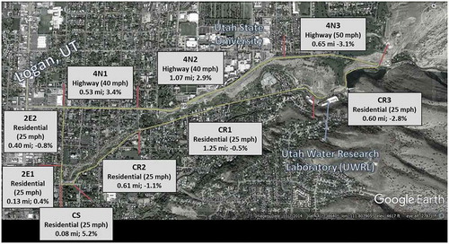
A route was developed over a variety of road types in Logan, UT, USA (see Figure 1). The chosen route contained different speed limits (25, 40, and 50 mph) and variable grades (uphill, downhill, and relatively flat segments). For analysis simplification, the route was divided into nine segments based on commonality of the above parameters as shown in Figure 1. Outside of exiting through the parking lot at the Utah Water Research Laboratory (UWRL), the volunteer drivers were not allowed to practice drive the test vehicle prior to their study drive.

Figure 1. Location of the selected route.

On-road tailpipe emissions of CO, HCs, and NO_x were monitored in real-time with an Autologic Applus 5-Gas Analyzer. The system was frequently calibrated with commercially available standard gases. It should be noted that tailpipe oxygen (O₂) and carbon dioxide (CO₂) were also measured, but these species will not be further discussed herein.

In addition to the pollutant measurements, several supporting parameters were also monitored in real-time. Engine RPM and other operating parameters were monitored using a commercial OBD scan tool. Previous to the on-road experiments, a linear algorithm was developed relating engine RPM to exhaust gas flowrate as measured by a propeller anemometer, accounting for the tailpipe cross-sectional area. This allowed the investigators to convert measured concentrations into units of mass flux. A Garmin eTrex GPS was used to monitor vehicle position, barometric pressure, and as a secondary measurement of vehicle speed. Finally, a series of type K thermocouples, wired to a Campbell Scientific datalogger, were used the monitor exhaust temperature and various other component temperatures (e.g., engine block, catalyst surface, etc.). During each drive, an investigator rode in the backseat of the test vehicle and monitored the data collection. A schematic representation of the system is shown in Figure 2.

Figure 2. Schematic of equipment setup.

Data processing and analysis

The Applus 5-Gas Analyzer reported the tailpipe gas concentrations in mixing ratios (ppm or volume percent). After each run, these mixing ratios were converted into mass concentrations (Seinfeld and Pandis 2016) and subsequently multiplied by the derived tailpipe exhaust flowrate to produce a mass per time emission rate (g/sec). Finally, the overall emissions in grams per mile (g/mi) were calculated by dividing the total emissions of the trip (g) by the total distance traveled (mi). All of the recorded data were collected at a frequency of 1 Hz.

For each run, across all road segments, the vehicle specific power, VSP, was also calculated to assess potential differences in this parameter along with the driver subgroups and the differences among the road segments. The VSP for light-duty vehicles is calculated as shown in eq 1 (Jiménez-Palacios 1999).

(1) $VSP=v\times \left[1.1a+9.81\times grade\left(\mathrm{\%}\right)+0.132\right]+0.000302\times v^3$(1)

where:

VSP = vehicle specific power (kW/t(metric))

v = vehicle speed (m/s)

a = vehicle acceleration (m/s²)

grade = vehicle vertical rise divided by the horizontal run (%)

A MATLAB code was developed to compile, organize, and analyze, as described above, the data from the four different data streams: the Applus emissions monitor, the temperature datalogger, the OBD scan tool, and the GPS system (refer to Figure 2). For the duration of each road test and throughout the nine route segments, the software code analyzed the individual driver results, the combined results for each target grouping, performed statistical analysis (ANOVA – analysis of variance), and produced the resultant graphs and tables.

Results and discussion

A representative example of the vehicle speed profile, compared to roadway elevation is shown in Figure 3. Additionally, the named roadway segments are also indicated. As shown, the roadway was segmented where there were consistent breakpoints in the driving routine, usually traffic control points or changes in grade or allowable speed limits. In addition, Figure 3 shows an overview look at concentration of the three pollutants (CO, HC, and NO_x) as the drivers move along the route for a typical driver. This figure shows that the concentrations vary considerably as the car moves along the route, especially the NO_x concentrations even for the same driver. The higher values of NOx are attributed to more loading of the engine, especially in the uphill and high-speed segments. The figure also shows the variability of the VSP along the route for that same driver.

Figure 3. Variations in elevation, speed, concentration of the three pollutants (CO, HC, and NO_x), and VSP in the route segments for a typical driver. Note: the bottom plot (VSP vs. position) is a binned plot that shows the median values and the inter-quartile range.

To test the statistical differences between emissions from young and experienced drivers, a simple one-way-ANOVA was performed. Figure 4 presents box-plots and the p-value for the F-statistic. If the p-value for the F-statistic is smaller than the significance level (usually 5%), then the test rejects the null hypothesis that all group means are equal and concludes that at least one of the group means is different from the others. The box-whisker plots of Figure 4 show that while there is no significant difference between the groups in terms of CO emissions, HC and NO_x emissions from experience drivers are significantly higher than those from the control driver, which is not the case for young drivers. This difference could be attributed to the fact that experienced drivers are more aggressive in general and tend to accelerate and load the engine more (Zheng et al. 2017). For the young drivers, the CO, HC, and NO_x emissions averaged 0.59 ± 0.69 g/mi, 0.060 ± 0.047 g/mi, and 0.083 ± 0.072 g/mi, respectively. While for the experienced drivers the same emissions averaged 0.888 ± 1.289 g/mi, 0.091 ± 0.072 g/mi, and 0.124 ± 0.132 g/mi, respectively. The uncertainty represents the 95% confidence interval about the mean.

Figure 4. CO, HC, and NOx results for young vs experienced drivers. On each box, the central mark indicates the median, and the bottom and top edges of the box indicate the 25th and 75th percentiles, respectively. The whiskers extend to the most extreme data points not considered outliers, and the outliers are plotted individually using the ’+’ symbol.

The second ANOVA test was performed to check the statistical differences between emissions from female and male drivers. As shown in Figure 5, emissions from male drivers are significantly higher than emissions from the control driver in terms of NO_x, and very nearly so for HC (p = .054). The male drivers were found to have CO, HC, and NO_x emissions averaging 1.00 ± 1.35 g/mi, 0.081 ± 0.049 g/mi, and 0.122 ± 0.141 g/mi, respectively. Comparatively, the female drivers were found to have emissions averaging 0.475 ± 0.317 g/mi, 0.071 ± 0.077 g/mi, and 0.085 ± 0.047 g/mi for CO, HC, and NO_x, respectively.

Figure 5. CO, HC, and NO_x results for male vs female drivers.

As can be seen in Figure 6, examination of the compiled data to the four target subject groups showed that there was no significant difference between the groups in terms of CO emissions. On the other hand, experienced male drivers were found to emit more HC and NO_x than the control driver. The box-whisker plots of Figure 6 also show that the variability among the young female was found to be the minimum across all of the pollutants. This may be attributed to the fact that in this group was the most homogeneous group in terms of age and driving experience. It also shows that the emissions in this group were the lowest because they may drive safer and at lower speed as suggested by Moè, Cadinu, and Maass (2015). The young female drivers were found to have average CO, HC, and NO_x emissions of 0.348 ± 0.276 g/mi, 0.046 ± 0.014 g/mi, and 0.085 ± 0.054 g/mi, respectively, while same emissions for the young male drivers averaged 0.832 ± 1.505 g/mi, 0.087 ± 0.093 g/mi, and 0.127 ± 0.160 g/mi, respectively. The experienced female drivers averaged CO, HC, and NO_x emissions of 0.603 ± 0.597 g/mi, 0.103 ± 0.166 g/mi, and 0.124 ± 0.078 g/mi, respectively, and experienced male drivers averaged 1.174 ± 3.106 g/mi, 0.089 ± 0.086 g/mi, and 0.206 ± 0.294 g/mi, respectively.

Figure 6. CO, HC, and NO_x results for the four groups.

Significant differences were noted among emissions from the target driver groups, with young and female drivers statistically showing the lowest emissions, particularly for NO_x and HC emissions. As previously referenced (Jiménez-Palacios 1999; Frey et al. 2015; Yao et al. 2013; Zhai et al. 2017; and others) and as was indicated in Figure 3, differences in on-road engine load in terms of Vehicle Specific Power (VSP) were reflected in difference in pollutant emissions. The overall VSP for each of the target driver groups was determined to look for insight on the observed emission differences. As can be seen in Figure 7, however, no significant differences were observed across the driver groups via ANOVA analysis (p = .1643). This is not unexpected as the designed roadway pattern included variable road types, speed limits, and grades with commensurate large variability in single driver VSP (−18.5–10.5 kW/t). More detailed examinations of the pollutant emissions and VSP values for different roadway segments for each of the driver groups were conducted in an attempt to more completely explain the observed differences.

Figure 7. Comparison of Overall VSP among the target driver group.

As previously discussed, the route was divided into nine segments based on stops, grade, and speed limit as was shown in Figures 1 and 3. Three representative segments, which were typically found to have high and low emissions, were chosen for further examination:

• 2E2, which is a 25 mph, residential, flat segment (−0.8 grade, 0.4 mi)

• 4N1, which is a 40 mph, highway, uphill segment (+3.4 grade, 0.53 mi)

• 4N3, which is a 50 mph, highway, downhill segment (−3.1 grade, 0.65 mi)

Confirming the differing engine workloads across the different road segments can be seen in the mean VSP as calculated for each of the road segments. As averaged across all driver groups, Figure 8 shows the uphill 4N1 segment had significantly higher VSP values, averaging 7.01 ± 0.82 kW/t and the downhill 4N3 had significantly lower VSP values, averaging −11.8 ± 0.76 kW/t, thereby supporting at least some the observed differences in the segmented pollutant emissions shown in Figure 9. The drivers on the flatter and slower road segment 2E2 were found to have an overall average VSP of −1.46 ± 0.14 kW/t.

Figure 8. Composite CO, NOx, and HC emissions for road segments 2E2, 4N1, and 4N3.

Figure 9. Comparison between VSP among the selected road segments.

Figure 9 shows that there were no significant differences in CO emissions among the three targeted segments. However, the HC emissions were significantly lower in the high speed, downhill 4N3 segment and the NOx emissions were significantly higher in the uphill, moderate speed 4N1 segment. As described by Kean, Harley, and Kendall (2003) and elsewhere, NOx emissions are known to increase as speed and engine load increase. Similarly, Pierson et al. (1996) and others have described increases in HC emissions as engine load decreased.

Tables 1–3 show comparisons of the mean VSP, pollutant emission rates, and the statistical level at which differences between the mean emission rates for each pollutant and each of the driver groups for roadway segments 2E2, 4N1, and 4N3, respectively. The “3σ” statistical significance guideline, or a 68% confidence interval, was used as the definition of acceptable significance. As an example, Table 1 shows that for road segment 2E2, average VSP for the five replicate drives by the control (Cntrl) driver was −1.47 kW/t, which was significantly different, at the 89% confidence level, from the experienced female (EF) driver group which showed an averaged VSP for the same road segment of −1.21 kW/t. From Table 1, it can also be seen that the EF group’s VSP mean was significantly lower than young female (YF) and experienced male (EM) driver groups.

Table 1. The average road segment 2E2 VSP and CO, NOx, and HC emission rates and statistical level at which the mean group emission rate becomes significantly different between the test groups. Note: Cntrl = control driver, YM = young male driver group, YF = young female driver group, EM = experienced male driver group, and EF = experienced female driver group.

Table 2. The average road segment 4N1 VSP and CO, NOx, and HC emission rates and statistical level at which the mean group emission rate becomes significantly different between the test groups. Note: Cntrl = control driver, YM = young male driver group, YF = young female driver group, EM = experienced male driver group, and EF = experienced female driver group.

Table 3. The average road segment 4N3 VSP and CO, NOx, and HC emission rates and statistical level at which the mean group emission rate becomes significantly different between the test groups. Note: Cntrl = control driver, YM = young male driver group, YF = young female driver group, EM = experienced male driver group, and EF = experienced female driver group.

Examining the CO, NOx, and HC emissions data shown in Table 1, ignoring comparisons with the Cntrl since the ultimate goal was to examine comparisons between the driver groups, it can be seen that the EF CO emissions were significantly different (higher) than the EM CO emissions. Similarly, the YF CO emissions were also found to be significantly higher the EM CO emissions. Furthermore, for road segment 2E2, there were no significant observed NOx emission differences, and only significant HC differences between the EF and YF driver groups. Recall, that of these differences, only the VSP values between the EM and EF driver groups were statistically different, suggesting the VSP differences along road segment 2E2 alone cannot account for differences in the observed emissions. It should also be noted here that using VSP-based emission algorithms developed by Rodríguez et al. (2016) for similar vehicle types produced emission rates generally within an order of magnitude of the values reported in Tables 1–3.

Table 2 shows the VSP values and pollutant emission rates for the higher speed, uphill road segment 4N1. The VSP values ranged from 6.16 kW/t (EM) to 8.12 kW/t (YF), and these two driver groups were the only one in which a significant difference (CI = 73.0%) was observed. Although only the single significant VSP difference was observed, the YF driver group was found to show lower CO emissions than the YM group, lower NOx emissions than the YM group, and lower HC emissions than the YM, EM, and EF groups. Additionally across the 4N1 road segment, the EF group show significantly lower CO emissions than the YM group. As with road segment 2E2, significant differences in VSP were not always reflected in significant emissions differences.

The comparisons for the downhill, higher speed road segment 4N3 are shown in Table 3. The YF and EF driver groups were shown to have lower VSP values compared to the YM group. However, like the roadway segments shown in Tables 1 and 2, the observed VSP differences did not consistently predict statistical differences in emissions between the driver groups. Over the 4N3 segment, the EF drivers were found to have significantly lower CO emissions than the EM drivers, no differences were observed in the NOx emissions, and the YF and YM drivers were found to average lower HC emissions the EM driver group.

Conclusion

To test the impacts of driver’s experience and gender and driving behavior on vehicular emission, an on-road emissions measurement experiment were performed in the city of Logan, UT, USA during the summer of 2016 wherein four different driver groups, driving the same vehicle over the same route were examined: female vs. male, experienced vs. inexperienced. The results showed that experienced drivers and male drivers emitted significantly more HC and NOx than the control driver, which was not the case for young and female drivers. Over the examined roadway segments it was found that young female drivers emitted on average 48% less HC and 58% less NOx than experienced male drivers. The study also showed that overall CO emissions were not significantly dependent on age, gender, nor driving conditions. The results also showed that the Vehicle Specific Power (VSP) was significantly different among the road segments but not among the all different groups. Furthermore, driving through low-speed segments emitted significantly higher HC, while driving through uphill segments emitted significantly higher NO_x. This is somewhat predicted in differences in engine load and resultant VSP.

Examination of individual road segments found more significant differences in some VSP and pollutant emissions, but the differences were not consistent across the examined road segments or target driver groups and did not consistently follow referenced relationship between VSP and emission rates (e.g., Rodríguez et al. 2016). The Young Female (YF) driver group, however, did tend to most frequently show statistically lower pollutant emission rates, especially for the uphill, high-speed road segment.

While the tested driver groups showed some statistical differences in driving behavior (VSP) and pollutant emissions, consistency of the significance was not observed. The study consisted of four categorized driver groups with four individuals in each group, and each individual drove the selected route a single time. To test for more robust statistical significance, a similar study should be initiated with a greater number of test individuals in each group and replicate, at least triplicate, tests for each individual. Although the data presented herein are not definitive, they do suggest that future modeling studies and regulatory scenarios should include gender profiles and driving experience to best estimate real-life, on-road mobile source emissions.

Additional information

Notes on contributors

Abdelhaleem I. Khader

Abdelhaleem I. Khader is an Assistant Professor of Civil and Environmental Engineering at An-Najah National University in Nablus, Palestine. He received his B.S. in Civil Engineering from An-Najah National University in 2004 and his M.S. in Water and Environmental Engineering from An-Najah National University in 2007, and his Ph.D. degree from Utah State University in Logan, Utah, USA in 2012.  He has been at An-Najah since the fall of 2013, prior to that he was a postdoctoral fellow at McMaster University in Hamilton, Ontario, Canada.  His recent research interests center around characterization of urban air quality using low-cost sensors and car emissions.  Dr. Khader’s expertise includes air quality monitoring, solid waste management, groundwater quality, and hydrological modeling.

Randal S. Martin

Randal S. Martin is a Research Associate Professor of Environmental Engineering at Utah State University with a joint appointment at the Utah Water Research Laboratory (UWRL), he also serves as an Associate Director of the Utah Climate Center and serves as a member of the state of Utah’s Air Quality Board.  He received his B.S. in Environmental Engineering at Montana Tech in 1982 and his M.S. and Ph.D. degrees from Washington State University in 1987 and 1992, respectively.  He has been at USU since the summer of 2000, prior to that he taught at New Mexico Institute of Mining and Technology in Socorro, NM.  His research interests center around the measurement and analysis of atmospheric trace species and area and mobile source emissions, most notably the characterization and behavior of ambient fine particulate matter (PM2.5 and PM10), reactive hydrocarbons and related oxidation products (esp. ozone).  Dr. Martin’s expertise includes air pollution photochemistry, air quality monitoring, biogenic emissions measurements, air pollution modeling, advanced oxidation processes for gaseous pollutant control, and source particulate fractionation and measurement.

References

- Ahn, K., H. Rakha, A. Trani, and M. Van Aerde. 2002. Estimating vehicle fuel consumption and emissions based on instantaneous speed and acceleration levels. J. Transp. Eng. 128 (2):182–90. doi:10.1061/(ASCE)0733-947X(2002)128:2(182).
- Austin, T. C., F. J. DiGenova, T. R. Carlson, R. W. Joy, and K. A. Gianolini. 1993. Characterization of driving patterns and emissions from light-duty vehicles in California. Final Report. PB-94-157005/XAB. ARBA932-185. Sacramento, CA: Sierra Research Corporation.
- Baldauf, R. W., C. Bailey, P. T. Rowley, M. Hoyer, and R. Cook. 2006. Impacts of traffic on air quality and health effects near major roadways. Presented at Urban Transport 2006, Prague, Czech Republic. July 12–14.
- Barlow, T. J., S. Latham, I. S. McCrae, and P. G. Boulter. 2009. A reference book of driving cycles for use in the measurement of vehicle road emissions. TRL Limited. Project Report PPR 354. Prepared for Department for Transport, Cleaner Fuels, & Vehicles, United Kingdom. ISSN: 0968-4093.
- Borken, J., H. Steller, T. Meréti, and F. Vanhove. 2007. Global and country inventory of road passenger and freight transportation, their fuel consumption and their emissions of air pollutants in the year 2000. Transp. Res. Rec. 2011. doi:10.314/2011/14.
- Borken-Kleefeld, J. 2013. Guidance note about on-road vehicle emissions remote sensing. Project report prepared for International Council on Clean Transport, San Francisco, CA, USA.
- Brundell-Freij, K., and E. Ericson. 2005. Influence of street characteristics, driver category and car performance on urban driving patterns. Transp. Res-Part D 10:213–29. doi:10.101/j.trd.2005.01.001.
- Dales, R., A. Wheeler, M. Mahud, A. M. Frescurs, M. Smith-Doiron, E. Nethery, and L. Liu. 2008. The influence of living near roadways on spirometry and exhaled nitric oxide in elementary school children. Environ. Health Perspect. 116 (10):1423–27. doi:10.1289/ehp.10943.
- De Genova, F., and T. C. Austin. 1994. Development of an onboard data acquisition system for recording vehicle operating characteristic and emissions. Fourth Annual CRC (Coordinating Research Council) On-Road Vehicle Emissions Workshop, March 14–16, 2014, San Diego, CA, USA, 3-59 to 3-82.
- De Vlieger, I. 1997. On-board emission and fuel consumption measurement campaign on petrol-driven passenger cars. Atmos. Environ. 31 (22):3753–61. doi:10.1016/S1352-2310(97)00212-4.
- De Vlieger, I., D. De Keukeleere, and J. G. Kretzschmar. 2000. Environmental effects of driving behavior and congestion related to passenger cars. Atmos. Environ. 34:4649–55. doi:10.1016/S1352-2310(00)00217-X.
- Ericsson, E. 2000. Variability in urban driving patterns. Transp. Res-Part D 5:337–54. doi:10.1016/S1361-9209(00)00003-1.
- Ericsson, E. 2001. Independent driving pattern factors and their influence on fuel-use and exhaust emission factors. Transp. Res-Part D 6:325–45. doi:10.1016/S1361-9209(01)00003-7.
- Franco, V., M. Kousoulidou, M. Muntean, L. Nziachristos, S. Hausberger, and P. Dilara. 2013. Road vehicle emission factors development: A review. Atmos. Environ. 70:84–97. doi:10.1016/j.atmosenv.2013.01.006.
- Frey, H. C., N. Rouphail, and H. Zhai. 2006. Speed and facility-specific emission estimates for on-road light-duty vehicles on the basis of real-world speed profiles. Transp. Res. Rec. 1987:128–37. doi:10.3141/1987-14.
- Frey, H. C., A. Unal, J. Chen, and S. Li. 2015. Evaluation and recommendation of a modal method for modeling vehicle emissions. Prepared by North Carolina State University for U.S. Environmental Protection Agency, San Diego. https://www3.epa.gov/ttnchie1/conference/ei12/mobile/frey.pdf (accessed March 2018).
- Frey, H. C., A. Unal, J. Chen, S. Li, and C. Xuan. 2002. Methodology for developing modal emission rates for EPA’s multi-scale motor vehicle & equipment emission system. EPA420-R-02-027, Prepared by North Carolina State University for U.S. Environmental Protection Agency, Ann Arbor, MI, USA.
- Granié, M. A., and E. Papafava. 2011. Gender stereotypes associated with vehicle driving among French preadolescents and adolescents. Transp. Res. Part F 14 (5):341–53. doi:10.1016/j.trf.2011.04.002.
- Holmén, B. A., and D. A. Niemeier. 1998. Characterizing the effects of driver variability on real-world vehicle emissions. Transp. Res-Part D 3 (2):117–28. doi:10.1016/S1361-9209(97)00032-1.
- Hung, W.-T., K.-M. Tam, C.-P. Lee, C.-P. Lee, L.-Y. Chan, and C.-S. Cheung. 2006. Characterizing driving patterns for Zhuhai for traffic emissions estimation. J. Air Waste Manag. Assoc. 56 (10):1420–30. doi:10.1080/10473289.2006.10464550.
- Jiménez-Palacios, J. L. 1999. Understanding and quantifying motor vehicle emissions with vehicle specific power and TLDAS remote sensing. PhD dissertation, Massachusetts Institute of Technology, Cambridge, MA, USA. Accessed March, 2018. http://hdl.handle.net/1721.1/44505.
- Kean, A. J., R. A. Harley, and G. R. Kendall. 2003. Effects of vehicle speed and engine load on motor vehicle emissions. Environ. Sci. Technol. 37 (17):3739–46. doi:10.1021/es0263588.
- Kelly, N. A., and P. J. Groblicki. 1993. Real-world emissions from a modern production vehicle driven in Los Angeles. J. Air Waste Manag. Assoc. 43 (10):1351–57. doi:10.1080/1073161X.1993.10467209.
- Koupal, J., M. Cumberworth, H. Micheals, M. Beardsley, and D. Brzezinski. 2003. Designing and implementation of MOVES: EPA’s new generation mobile source emission model. Presented at the International Emission Inventory Conference “Emission Inventories – Applying New Technologies. San Diego, CA, USA. Available https://www3.epa.gov/ttnchie1/conference/ei12/mobile/koupal.pdf (accessed March 2018).
- Li, Q., F. Qiao, and L. Yu. 2016. Vehicle emission implications of drivers’ smart advisory system for traffic operations in work zones. J. Air Waste Manag. Assoc. 66 (5):446–55. doi:10.1080/10962247.2016.1140095.
- Liu, B., and H. C. Frey. 2015. Variability in light-duty gasoline vhecile emission factors from trip-based real-world measurements. Environ. Sci. Technol. 49 (20):12525–34. doi:10.102/acs.est.5b00553.
- Moè, A., M. Cadinu, and A. Maass. 2015. Women drive better if not stereotyped. Accid. Anal. Prev. 85:199–206. doi:10.1016/j.aap.2015.09.021.
- Özkan, T., and T. Lajunen. 2006. What causes the differences in driving between young men and women? The effects of gender roles and sex on young drivers’ driving behaviour and self-assessment of skills. Transp. Res. Part F 9 (4):269–77. doi:10.1016/j.trf.2006.01.005.
- Park, S. S., K. Kozawa, S. Fruin, S. Mara, Y.-K. Hsu, C. Jakober, A. Winer, and J. Herner. 2011. Emission factors for high-emitting vehicles based on on-road measurements of individual vehicle exhaust with a mobile measurement platform. J. Air Waste Manag. Assoc. 61 (10):1046–56. doi:10.1080/10473289.2011.595981.
- Pierson, W. R., A. W. Gertler, and R. L. Bradow. 1990. Comparison of the SCAQS tunnel study with other on road vehicle emission data. J. Air Waste Manag. Assoc. 40 (11):1495–504. doi:10.1080/10473289.1990.10466799.
- Pierson, W. R., A. W. Gertler, N. F. Robinson, J. C. Sagebiel, B. Zielinska, G. A. Bishop, D. H. Steadman, R. B. Zweidinger, and W. D. Ray. 1996. Real-world automotive emissions – Summary of studies in the Fort McHenry and Tuscarora tunnels. Atmos. Environ. 30 (12):2233–56. doi:10.1016/1352-2310(95)00276-6.
- Robert, M. A., S. VanBergen, and M. J. Kleeman. 2007. Size and composition distributions of particulate matter emissions: Part 1—Light-duty gasoline vehicles. J. Air Waste Manag. Assoc. 57:1414–28. doi:10.3155/1047-3289.57.12.1414.
- Rodríguez, R., E. A. Virguez, P. A. Rodríguez, and E. Behrentz. 2016. Influence of driving patterns on vehicle emissions: A case study for Latin American cities. Transp. Res-Part D 43:192–206. doi:10.1016/j.trd.2015.12.008.
- Ross, M., R. Goodwin, R. Watkins, T. Wenzel, and M. Q. Wang. 1998. Real-world emissions from conventional passenger cars. J. Air Waste Manag. Assoc. 48 (6):502–15. doi:10.1080/10473289.1998.10463705.
- Seinfeld, J. H., and S. N. Pandis. 2016. Atmospheric chemistry and physics: From air pollution to climate change, 10–12. 3rd ed. Hoboken, NJ: John Wiley & Sons.
- Smit, R., L. Nziachristos, and P. Boulter. 2010. Validation of road vehicle and traffic emission models – A review and met-analysis. Atmos. Environ. 44:2943–53. doi:10.1016/j.atmosenv.2010.05.022.
- Tong, H. Y., W. T. Hung, and C. S. Cheung. 2000. On-road motor vehicle emissions and fuel consumption in urban driving conditions. J. Air Waste Manag. Assoc. 50 (4):543–54. doi:10.1080/10473289.2000.10464041.
- UDOT. 2016. License drivers by age and sex. United States Department of Transportation Federal Highway Administration. Office of Highway Policy Information. Accessed February, 2018. https://www.fhwa.dot.gov/ohim/onh00/bar7.htm.
- UDOT. 2018. Table 1-11. Number of U.S. aircraft, vehicles, vessels, and other conveyances. United States Department of Transportation Bureau of Transportation Statistics. Accessed February 2018. https://www.rita.dot.gov/bts/sites/rita.dot.gov.bts/files/publications/national_transportation_statistics/html/table_01_11.html.
- USEPA. 2016. Number of people living in counties with air quality concentrations above the level of the NAAQS in 2015. United States Environmental Protection Agency. Accessed August, 2016. https://www.epa.gov/sites/production/files/2016-06/ctypeoplechart2015.png.
- USEPA. 2017. Air pollution emissions trends data: Average annual emissions. United States Environmental Protection Agency. Air Emissions Inventories. Accessed February, 2018. https://www.epa.gov/vehicle-and-fuel-emissions-testing/dynamometer-drive-schedules.
- USEPA. 2018. Dynamometer drive schedules. United States Environmental Protection Agency. Vehicle and Fuel Emissions Testing. Accessed March 2018. https://www.epa.gov/air-emissions-inventories/air-pollutant-emissions-trends-data.
- Utah Division of Air Quality (UDAQ). 2019. Personal communication. Joe Thomas, Inventory Branch, Environmental Program Manager, Salt Lake City, Utah, April 12.
- Wang, H., and L. Fu. 2010. Developing a high-resolution vehicular emission inventory by integrating an emission model and a traffic model: Part 1—Modeling fuel consumption and emissions based on speed and vehicle-specific power. J. Air Waste Manag. Assoc. 60:1463–70. doi:10.3155/1047-3289.60.12.1463.
- Wasielewski, P., and L. Evans. 1985. Do drivers of small cars take less risk in everyday driving? Risk Anal. 5 (1):25–32. doi:10.1111/risk.1985.5.issue-1.
- WHO. 2015. Global status report on road safety. World Health Organization. Accessed March, 2018. http://www.who.int/violence_injury_prevention/road_safety_status/2015/en/. ISBN 978 92 4 156506 6.
- WHO. 2016. Ambient (outdoor) air quality and health: Fact sheet. World Health Organization. Media Center. Accessed February, 2018. http://www.who.int/mediacentre/factsheets/fs313/en/.
- Wyatt, D. W., H. Li, and J. E. Tate. 2014. The impact of road grade on carbon dioxide (CO2) emissions of a passenger vehicle in real-world driving. Transp. Res-Part D 32:160–70. doi:10.1016/j.trd.2014.07.015.
- Yao, Z., H. Wei, H. Liu, and Z. Li. 2013. Statistical vehicle specific power profiling for urban freeways. Presented at the 13th COTA International Conference of Transportation Professionals (CICTP 2013). Procedia Soc. Behav. Sci. 96:2927–38. doi:10.1016/j.sbspro.2013.08.324.
- Yu, L. E., L. M. Hildemann, and W. R. Ott. 1996. A mathematical model for predicting trends in carbon monoxide emissions and exposures on urban arterial highways. J. Air Waste Manag. Assoc. 46 (5):430–40. doi:10.1080/10473289.1996.10467476.
- Zhai, H., H. C. Frey, and N. M. Rouphail. 2011. Development of a modal emissions model for a hybrid electric vehicle. Transp. Res-Part D 16 (6):444–50. doi:10.1016/j.trd.20141.05.001.
- Zhai, Z., G. Song, H. Lu, W. He, and L. Yu. 2017. Validation of temporal and spatial consistency of facility- and speed-specific vehicle-specific power distributions for emission estimation: A case study in Beijing, China. J. Air Waste Manag. Assoc. 67 (9):949–57. doi:10.1080/10962247.2017.1294545.
- Zheng, F., J. Li, H. Van Zuylen, and C. Lu. 2017. Influence of driver characteristics on emissions and fuel consumption. Transp. Res. Procedia 27:624–31. doi:10.1016/j.trpro.2017.12.142.