Observed ozone over the Chesapeake Bay land-water interface: The Hart-Miller Island Pilot Project

ABSTRACT

Enhanced ozone concentrations at land-water interfaces create National Ambient Air Quality Standard (NAAQS) compliance issues across the United States. The northern Chesapeake Bay experiences higher ozone at sites adjacent to the Bay, creating ozone compliance concerns for the state of Maryland. Accordingly, the Maryland Department of the Environment sited an ozone monitor at Hart-Miller Island (HMI) within the northern Chesapeake Bay (NCB) and gathered a continuous ozone and meteorological record over 278 days within the 2016 and 2017 ozone seasons. The representative water site was the highest ozone monitor in the state 28% of all days and 75% when any ozone monitor in the state experienced ozone above the 2015 ozone NAAQS (70 ppbv), known as an exceedance day. In total, 24 exceedance days were observed at HMI. Numerical ozone predictions produced by an operational version of the Community Multi-scale Air Quality (CMAQ) model forecast 52 such days with a high bias of 15.5% in daily maximum ozone concentration during the same period. Trajectory modeling indicated over 70% of exceedance days possessed northwesterly transport over the Baltimore area, with HYSPLIT trajectories descending at least 500 m in greater than 80% of cases toward the NCB surface. These trajectories possessed a button-hook pattern during descent to create southerly surface winds at HMI that may impact coastal sites, creating ozone events at Maryland monitors such as Edgewood. Consequently, the NCB was influenced by the residual layer and from both regional long-range transport and locally sourced ozone precursors. Changes in local meteorology and emissions had a significant impact on over-water ozone concentrations and forecasts. Results of the multi-season ozone pilot study over the Chesapeake Bay provided a conceptual model of high ozone development over water downwind of a large urban center and guidance for future study of the NCB area.

Implications: Multi-seasonal observations of surface ozone and meteorology over the water of the northern Chesapeake Bay showed specific conditions leading to degraded air quality. The novel data set collected offers a deeper understanding of over-water ozone magnitude, occurrence, and transport across the land-water interface and comparison to air quality models not before possible.

Introduction and motivation

Tropospheric ozone is a federally regulated pollutant impacting human health and causing environmental stress. National Ambient Air Quality Standards (NAAQS) set by the United States (U.S.) Environmental Protection Agency (EPA) establish pollutant thresholds which must be met by state and tribal regulatory agencies. Ozone and ozone precursors have been in significant decline over the past decade (Aburn et al. 2015), yet ozone at land-water interfaces continue to present unique air quality challenges. Locations in the U.S. near bodies of water such as Lake Michigan, the Long Island Sound, South Coast, CA, Houston, and the Chesapeake Bay observe and/or model ozone concentrations in excess of the NAAQS. As of 2010, 123.3 million people (39% of the U.S. population) lived in coastal areas with an additional 10 million projected by 2020 (Crossett et al. 2013). Enhanced ozone near these locations exposes this large population to the health impacts of degraded air quality. Despite reductions in the ozone precursors Nitrogen Oxides (NOx = NO2 + NO) and Volatile Organic Compounds (VOCs), 21 coastal areas remain in non-attainment status of the EPA’s 2015 70 ppbv ozone standard. Modeling also projects concentrations above 70 ppbv in future years at monitors near these land-water interfaces (e.g., Ring et al. 2018; Vinciguerra et al. 2017). Observations at these land-water interfaces are therefore vital for evaluating science and policy, as well as for human and environmental health.

Maryland ozone monitors adjacent to the northern Chesapeake Bay (NCB, i.e., the Chesapeake Bay north of 39°N latitude) comprise most monitors not attaining the 2015 ozone NAAQS. The Edgewood, Maryland ozone monitor, for example, had the highest ozone design value (a three-year average of the fourth-highest maximum daily eight-hour ozone concentration) between 2008 and 2013 of all ozone monitors along the United States’ east coast. Marine air over the Bay was implicated for higher ozone concentrations at near-water monitors compared to nearby in-land monitors (Landry 2011) and a reason current observations keep NCB coastal monitors in non-attainment of the 2015 EPA standard. Policy modeling of future year design values using the EPA Community Multi-scale Air Quality (CMAQ) model also projects continued non-attainment at NCB coastal sites. If Maryland non-attainment is due to ozone formation over the NCB moving ashore within land-water thermally induced “bay breezes”, ozone in excess of 70 ppb should be observable over the water prior to impacting coastal sites. Previous observational work confirmed higher ozone concentrations over the Chesapeake Bay than nearby land sites (e.g., Goldberg et al. 2014; Stauffer et al. 2015) but was length-limited for policy application. A longer, persistent record was needed to understand the development of ozone over the NCB and its regulatory impact on these non-attainment coastal sites. While the focus is on the NCB, the scope of the findings presented here has significance for other coastal regions.

Differential heating between land and water is responsible for land-water breeze development around water bodies, the underlying assumed cause of Maximum Daily 8-hour Average Ozone (MD8AO) above the 70 ppbv 2015 ozone NAAQS (henceforth “exceedance day”) at coastal sites. Land-water breezes have been a long-studied phenomenon (e.g., Biggs and Graves 1962; Frysinger, Lindner, and Brueske 2003; Laird et al. 2001; Miller and Keim 2003; Porson, Steyn, and Schayes 2007), as have their impact on air quality (e.g. Lennartson and Schwartz 2002; Lyons 1972; Martins et al. 2012). Referred to as “bay breezes” around the Chesapeake Bay, their impacts on air quality there have also been noted (Goldberg et al. 2014; Landry 2011; Loughner et al. 2014; Sikora, Young, and Bettwy 2010; Stauffer et al. 2015). Martins et al. (2012) found exceedance days were highly correlated to bay breezes in the coastal area near Hampton, Virginia in the southern Chesapeake Bay. They also noted seasonal differences in mean meteorology influenced the number of ozone exceedance days and the number of bay breeze events. Daily and seasonal meteorological influences on bay breeze formation were also evident over the NCB, but bay breeze formation alone did not solely identify exceedance days at those coastal sites.

EPA requires state ozone design values be at or below 70 ppbv to demonstrate attainment of the ozone NAAQS. For coastal areas, investigation of new ozone reduction strategies requires understanding the reasons driving the continued observed and modeled non-attainment. Many factors contribute to the spatial and temporal complexity of ozone distribution around the NCB. Ozone precursors from local emissions in the Washington DC-Baltimore corridor are additive to transported pollution from out of state, which while in significant decline in recent years (Gégo et al. 2007), may add sufficient burden for ozone exceedance days (Aburn et al. 2015). Understanding the spatiotemporal variability and contribution of local emissions to ozone is important for guiding control strategies, but any such strategy needs a conceptual model of land-water interface transport evolution on exceedance days over the NCB. In-situ observations are thus required to identify the circumstances of exceedance days. Once identified, probable source regions of precursor emissions may be located with trajectory analyzes on these exceedance days while meteorological information provides further context and explanation. Local and long-range precursor transport are quantified by aloft measurements in the context of reported emissions. Meteorological and anthropogenic conditions leading to instances of NCB ozone in excess of the NAAQS and any subsequent impacts on land, ozone attainment, and human health may be explained through such retrospective analysis and compared to numerical modeling. However, no such undertaking was possible without a viable, long-term record of over-water measurements.

Model verification over the NCB has immediate application and implications for air quality forecasting, policy, and attainment modeling. However, numerical guidance verification over water is sparsely attempted due to logistical difficulties associated with observations. Apart from short-term intensive research campaigns such as the Deriving Information on Surface Conditions from Column and Vertically Resolved Observations Relevant to Air Quality (DISCOVER-AQ) 2011 campaign in Maryland, surface observations over water are few. Numerical simulations of ozone consistently predict enhanced surface ozone concentrations over the NCB. The non-regulatory, operationally driven daily forecast guidance provided by the National Oceanic and Atmospheric Association (NOAA) CMAQ model was high biased at land sites due to adjacent high ozone at over-water grid cells (Figure 1). Whether high ozone at coastal grid cells was an artifact of the model resolution or a mishandling of reality was unclear. A similar predicament exists within the regulatory version of CMAQ driving state compliance modeling used to calculate future year design values. Prior future year projections were higher than what was later observed at coastal sites. Future year predicted non-attainment is driven by modeled high ozone over water. Previously, verification of modeled enhanced ozone over the NCB surface was only assumed when winds off the NCB impacted a nearby coastal site. Potential verification of exceedance days at coastal sites were irregular and relatively unpredictable. In-situ observations over the NCB would enable a more thorough comparison to models and test high ozone forecast there.

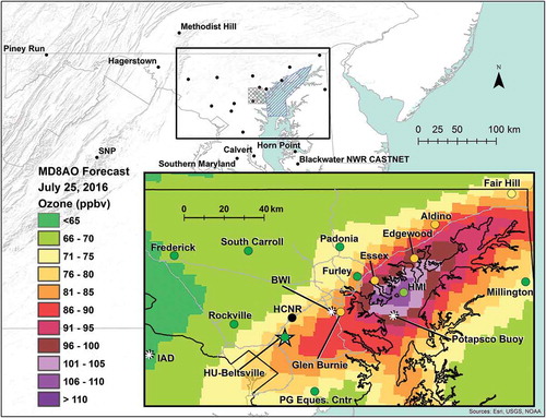
Figure 1. Map of the experimental domain and example CMAQ forecast model output compared to monitored concentrations. Background map: Large scale view of the region. Black dots are ozone monitors within the Maryland ozone network or specifically mentioned through the text, annotated with names when outside the inset map region. The gray cross-hatched area defines the southern Baltimore NOx heavy region mentioned in the text. The Northern Chesapeake Bay (NCB) referred to in the text is defined by the blue hatched area. The study domain and inset map area are defined by the black rectangle. Inset Map: The Maryland ozone monitoring network (circles) are colored by observed maximum daily 8-hour average ozone (MD8AO, ppbv) superimposed on forecast MD8AO from the NOAA operational CMAQ model, 7 am (1200 UTC) run (contoured colors, ppbv) on July 25, 2016. Radar Wind Profilers (RWP) are labeled with stars at collocated monitors. Gray lines are major interstates. Ozone is not measured at the HCNR site (black shading). Forecast MD8AO at Hart-Miller Island (HMI) was 107 ppbv on July 25, 2016 but instrumentation observed 70 ppbv, demonstrating the numerical prediction difficulties of ozone pollution over water, epitomizing the over-water ozone issue.

The Maryland Department of the Environment (MDE) Air Monitoring Program deployed ozone monitoring equipment to the Hart-Miller Island (HMI) site for two summer seasons in 2016 and 2017 to investigate ozone over the NCB. The resulting continuous seasonal datasets of ozone and meteorology allowed an investigation of the frequency, meteorological conditions conducive to, transport, model verification, and emissions during ozone exceedance days over the NCB not before available. The analysis presented here conceptualizes the conditions fostering exceedance days over the two seasons of study. A brief description of the unique observation platform and site used in this study is presented first followed by a description of the non-regulatory CMAQ forecasts used to compare MD8AO. Observational results are summarized next. Conditions leading to ozone exceedance days of the 2015 ozone standard are also examined followed by comparison to model forecasts. Hypotheses addressing phenomena controlling ozone in the NCB are addressed in the discussion and conclusions.

Portable ozone monitor on Hart-Miller Island

MDE deployed a portable ozone monitor (“HMIPOM”) on HMI within the NCB. HMI was an 1100 acre island located approximately 22 km east of downtown Baltimore, roughly 5 km from the main Maryland shore (Figure 1). The HMIPOM was sited at the northeastern most point of the island (39.2572°N, 76.3446°W) on the upper portion of the island retaining dike, approximately 13 m above water level. This site provided a prominent and exposed position near the center of the NCB, representative of the over-water air shed, and within an area where the NOAA operational CMAQ model often projected high ozone (e.g., Figure 1). The HMIPOM was operational 82 days between its placement (July 6) and retrieval (October 4) in 2016 and 211 days (April 13 – November 9) during the 2017 season. Since 2008, 95% of all exceedance days in the state of Maryland fell between May and September with the peak exceedance day period occurring in June and July.

Equipment on the HMIPOM included a 2B Technologies, Inc. (Boulder, CO, USA) ozone monitor (Model 202) and Vaisala WXT536 meteorological instrument, which measured approximately 2.4 and 3 m, respectively, above ground level (AGL). Meteorological parameters included wind, temperature, pressure, humidity, solar irradiance, and precipitation. All federal guidelines were met in the construction and quality control of the HMIPOM, allowing it to be considered a federal equivalent method (FEM) comparable to other Maryland FEM and FRM (federal reference monitor) ozone measurements. Weekly precision checks against a certified level 3 ozone calibrator averaged +0.46% bias over the two seasons.

The NOAA CMAQ model

The National Air Quality Forecast Capability (NAQFC) supported by NOAA provides a chemical forecast across the Continental United States, Alaska, and Hawaii. The NAQFC forecasting system is comprised of an offline coupling of the official North American Mesoscale Forecast System (NAM) and CMAQ using a 12 km horizontal grid spacing. Colloquially referred to as the NOAA CMAQ, the model is a non-regulatory version of CMAQ designed for support of daily operational decision making by providing daily numerical ozone predictions. This model is useful to compare with observations at HMI because of its continuous daily record over multiple years, accessibility, availability, and applicability to air quality forecasting. Daily forecast output was retrieved from the NOAA Operational Model Archive and Distribution System (NOMADS). Numerical ozone forecasts of same-day MD8AO were extracted from the 7 am EST CMAQ initialization model grid cell encompassing the HMIPOM for each MD8AO observation at HMI over the two seasons. The model output was then compared to MD8AO observed at HMI.

Chemistry

The NOAA CMAQ is a specifically configured chemical transport model built from the publicly released EPA software package available from the Community Modeling and Analysis System (CMAS). The CMAQ model version changed from 4.6 to 5.0.2 on June 14 2017 (CMAQ version numbers refer to the EPA version number). In the change, the total advection-subjected species increased from 135 to 157. The major difference in the configuration between these two versions of the NOAA CMAQ laid in the gas-phase mechanism. The gas-phase mechanism was upgraded with improved VOC reactions, particularly with the implicit expressions of the toluene and xylene species. The inclusion of their detailed reaction with chlorine radicals tended to deplete hydroxyl radicals for ozone production and was thought to help reduce the high-bias forecast of surface ozone. Additionally, the so-called organic nitrate (NTR) species responsible for radical recycling in the production of ozone had its total reactivity reduced by splitting the NTR species into seven more explicit species (Sarwar et al. 2013; Schwede, D. CMAS 2014,; Lee et al. 2017). The increase of sophistication in modeling the organic nitrate species was believed to be the primary cause to reduce the overly reactive NTR contribution of ozone production modeled in CMAQ 4.6.

The NOAA CMAQ configuration used the cb05 gas chemistry mechanism. Aerosol chemistry was upgraded from aero4 to aero6 in the 2017 model upgrade. The photolysis rates were all calculated inline utilizing the CMAQ so-called JPROC module based on a tropospheric ultraviolet (TUV) radiative transfer model. Aqueous phase reactions and optical properties calculated were all specified using default options of CMAQ. All other removal and deposition processes had their recommended default setting applied. Newer CMAQ versions starting from version 5.1 include detailed halogen chemistry advantageous to reduce the over-prediction of surface ozone in coastal cities. The NAQFC team was aware of the availability of newer versions of CMAQ, however CMAQ 5.1 was undergoing pre-implementation studies and being evaluated in operational forecasting settings for potential upgrades to the NOAA CMAQ and was therefore not implemented during the HMI pilot project.

Emissions

The U.S. EPA 2011 National Emission Inventory (NEI) version 2 was incorporated into the NAQFC emission projections as baseline emission flux strengths across various sectors. The emission projection methodology is practically considered due to operational forecast constraints. All inventory data were processed using the U.S. EPA Sparse Matrix Operator Kernel Emissions (SMOKE) Modeling System to represent monthly, weekly, daily and holiday/non-holiday variations specific for the forecast year. Point sources, which represent energy generation units (EGU) and other large prominent sources, were projected with observational data acquired within months prior to the forecast time. The EGU and non-EGU U.S. nitrogen oxides (NOx) and sulfur dioxide (SO2) point source strengths were also obtained from EPA. These point sources were updated with the 2014–2015 Continuous Emission Monitoring (CEM) biennial database. EGU projections were computed using the ratios of the emission strengths between measured past years to the forecast year after consulting with the Department of Energy’s energy consumption projection for the forecast year. Mobile sources were a combination of area and line sources. The on-road emission inventory was projected based on the EPA Cross State Air Pollution Rule (CSAPR) (available at: https://www.epa.gov/csapr). Natural and mobile sources were meteorologically modified using the same NEI base year. Biogenic emissions and plume rise for point sources are all inline as the CMAQ version recommends.

The 2011 NEI version 2 was also used for all agricultural ammonia (NH3), railway, class 1 and 2 marine emissions primarily representing non-ocean-going activities, vehicular refueling, oil and gas industry related emissions, residential wood combustion, and off-road emissions. Emissions from wildfires, prescribed agricultural burns, and land clearing fires based on climatology were removed from the area source emissions and replaced with dynamic fire emission forecasting using a version of the U.S. Forest Service BlueSky smoke emission package and the NOAA/NESDIS Hazard Mapping System (HMS) for fire locations and strength. Gas-phase chemistry from wildfire smoke was not included in ozone reactions. The wind-blown dust module was set to use the Fengsha module and sea-salt spray module was set to use the standard defaults accompanied by standard ocean files applicable for NAQFC during the study periods. For offshore large point sources, the U.S. EPA 2008 offshore emission inventory was used.

Meteorology and data assimilation of meteorological observations

The NOAA CMAQ uses forecast meteorology from the NAM, a major variation from meteorology used in retrospective State Implementation Plan (SIP) assessment applications of the CMAQ model. The NAM is based on the Non-hydrostatic Multiscale Model (Janjić and Gall 2012) with Arakawa B grid-staggering (NMMB) model covering all 50 states and territories of the U.S. As the nation’s official meteorological forecast model, it has access to the most comprehensive meteorological data assimilation and observation acquisition systems available. Regional data assimilation systems were used to assimilate meteorological and land-surface observational data and provide initial conditions: NAM Data Assimilation System (NDAS) (Wu, Purser, and Parrish 2002), and the NCEP Oregon State University, Air Force and Hydrologic Research Laboratory (Noah) Land Surface Model (LSM) based Data Assimilation System (NLDAS) provides land states (Mitchell et al. 2004). The Mellor-Yamada-Janjić planetary boundary layer (PBL) was used to determine the boundary layer height that was used as a governing parameter for determining the convective mixing of pollutants by the Asymmetrical Convective Model (Pleim 2007).

Results

General ozone observations on HMI

Observations at HMI showed the NCB susceptible to ozone in excess of the NAAQS more frequently than other sites but also that the island site was not consistently highest in the state, even when other monitors experienced exceedance days. Overall the HMI site was the highest monitor in the state on 28% of the 278 days with a valid MD8AO. The HMIPOM recorded 24 exceedance days, 13 and 11 during the 2016 and 2017 ozone seasons, respectively, though the HMIPOM was the highest monitor in Maryland on 18 of the 24. Six exceedance days occurred solely at HMI, but there were also nine days the NCB did not have MD8AO exceeding 70 ppbv even though other exceedance days occurred at other Maryland monitors (e.g., Figure 1).

There were 125 days identified in the study period with a maximum temperature at Baltimore-Washington International Airport (BWI, 39.177°N, 76.667°W; 29 km WSW of HMI) equal to or greater than 85°F. The temperature-ozone correlation has been well established (e.g. Bloomer, Konstantin, and Dickerson 2010; Rasmussen et al. 2012) and BWI provided meteorological data over land to compare to the HMI site. BWI has also historically served as a regional meteorological reference for analyzes conducted by the state of Maryland. Among days ≥85°F at BWI, the HMIPOM had the highest MD8AO in the state ~35% of the time. Thus, even during warm days, the HMIPOM did not consistently report the highest ozone concentration in the state.

Meteorological differences account for the greater number of exceedance days in 2016 despite a shorter observation period. While the HMIPOM was deployed there were 41 days of maximum temperatures at BWI of at least 90°F in 2016 with only 31 in 2017. Slightly cooler overall temperatures in 2017 (85.3°F vs. 84.2°F for JJA in 2016 and 2017, respectively) were accompanied by overall slightly windier conditions based on North American Regional Reanalysis data (retrieved from the NOAA Physical Sciences Division). Northwest synoptic flow within the boundary layer, representing an orthogonal component to the NCB, had a similar frequency between the years (31% in 2016 and 35% in 2017 of all study days of each year). However, during days with ≥85°F at BWI, trajectories came from the northwest 23 of 27 days in 2016 and 22 of 53 days in 2017. The contextual importance of this finding will be elaborated later.

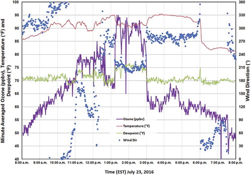
Enhanced ozone at HMI occurred primarily with southerly winds with intense gradients suggested by 10+ ppbv changes accompanied by wind shifts (Figure 2). In a dramatic example, 5-minute averaged ozone concentrations at the HMIPOM on July 23, 2016 increased from 68 ppbv at 1:11 pm Eastern Standard Time (EST) with winds from 276° to 93 ppbv with winds from 218° at 1:24 pm EST. Ozone later dropped with a similar wind shift in reverse going from 84 ppbv to 66 ppbv between 2:55 and 3:02 EST as winds changed from 213° to 290°. The wind speed increased from an average of 6.6 mph from 12:40 pm to 1:11 pm to 9.0 mph between 1:11 pm and 2:57 pm EST, with a 1-minute maximum of 13.3 mph (1:28 pm) as ozone concentrations peaked. As was the case on July 23, 2016, wind shifts associated with greater ozone were also, in general, accompanied by decreased temperature and increased dewpoint characteristic of marine air.

Figure 2. Minute average temperature (°F, red line), dewpoint (°F, green line), wind direction (°, blue dots) and ozone (ppbv, purple line) at Hart-Miller Island (HMI) on July 23, 2016. Ozone both increased and decreased by approximately 20 ppbv with shifts in wind direction accompanied by a drop in temperature and increase in dewpoint.

Ozone over the NCB exhibited an apparent weekly cycle (Table 1). Considering all days over the two seasons, MD8AO at HMI peaked on Wednesday and was lowest on Sunday with an 8.3 ppbv difference between the daily means. However, statistical tests failed to show significance between any days, even the large apparent disparity between Sunday and Wednesday. Ozone observed at HMI correlated most closely with Essex (r = 0.973) and least with the EPA Blackwater NWR CASTNET monitor (r = 0.637) on the southern Eastern Shore of Maryland. Essex, which was also the closest spatially to HMI, mimicked the average weekly pattern of all study days but remained 2.6–4.5 ppbv lower. Ten of the 21 sites across the state also peaked on Wednesday with the other 11 peaking on Thursday. The lowest average ozone during the week fell on either Saturday or Sunday at 14 of 21 monitors.

Table 1. Day of the week average ozone concentration at Hart-Miller Island for all valid Maximum Daily 8-hour Average Ozone (MD8AO) days in 2016 and 2017 and all valid MD8AO days with a maximum temperature ≥85°F at BWI airport in 2016 and 2017. Standard deviations and number of samples for each data set are also provided. The number of times HMI had Maximum Daily 8-hour Average Ozone (MD8AO) in excess of 70 ppbv per day of the week is provided in the final column. The highest concentrations occurred midweek. Sundays observed the lowest concentrations and exceedances.

	Ozone [ppbv]
	All Days			Max Temp ≥85°F			MD8AO
Day of the week	Mean	St. Dev	Samples	Mean	St. Dev	Samples	>70 ppbv
Sunday	48.5	10.9	36	54.5	11.4	18	1
Monday	52.1	14.5	35	60.1	11.9	17	3
Tuesday	53.5	15.0	35	64.3	13.1	16	5
Wednesday	56.8	17.1	36	64.2	17.2	20	6
Thursday	54.9	11.4	36	60.4	10.9	18	3
Friday	52.2	14.7	36	60.5	15.3	17	4
Saturday	50.6	12.3	36	58.3	9.9	19	2

Considering only days with a maximum temperature ≥85°F at BWI, day of the week ozone distribution was similar to all days with no statistical significance between days. Essex again had the highest correlation to the HMIPOM among these days (0.975) but remained 2.8–4.8 ppbv lower. Of 21 Maryland sites 15 reached their peak on either Tuesday or Wednesday. Saturday and Sunday exhibited the lowest amount of ozone at HMI with a nearly 10 ppbv disparity between Tuesday and Sunday. Other sites in Maryland observed a similar pattern, with 17 of the 21 sites observing their lowest concentrations over the weekend, with 16 on Sunday alone. The lowest average temperature in this group occurred on Sunday (89.6°F) and greatest was Friday (91.8°F).

Mean diel profiles

Mean hourly ozone concentration by hour of the day for all observation days indicated the largest differences between HMI and nearby NCB coastal monitors were during pre-dawn hours and on exceedance day afternoons. Over all days, ozone remained as much as 12 ppbv greater overnight at HMI than the nearest land sites (i.e., Edgewood, Essex, and Glen Burnie, c.f. Figure 1) and concentrations over the NCB were 4–5 ppbv higher than the next highest monitor by late afternoon (4–5 pm EST).

Greater ozone concentrations and faster ozone increases were noted during warm days (BWI maximum temperature ≥85°F) and on exceedance days (Figure 3). Interestingly, while there was greater ozone during warm non-exceedance days at HMI compared to the average of all days, ozone concentrations declined through the afternoon at both HMI and land sites (Figure 3a). In contrast, exceedance day profiles exhibited sustained and increasing ozone concentrations after 12–1 pm EST (Figure 3b). The differences were most pronounced at HMI where the ozone peak at 3 pm EST was 9.4 ppbv greater than the next highest nearby land site.

Figure 3. Diel profiles of ozone concentration averaged by hour at HMI and the surrounding MDE sites of Essex, Glen Burnie and Edgewood for (a) non-exceedance days at HMI with “warm” (≥85°F) temperatures at BWI [100 days] and (b) for those days where HMI had a maximum 8-hour average ozone greater than 70 ppbv [24 days]. Diel profiles of hourly rates of change (ppbv/hr) in (c) for the non-exceedance days found in (a), and (d) the exceedance days at HMI from (b).

Diurnal ozone increases were delayed and initially slower at HMI than nearby land sites on both warm non-exceedance days (Figure 3c) and exceedance days (Figure 3d). While early morning ozone concentrations at HMI were notably higher than adjacent land sites, ozone concentrations at land sites matched that at HMI by mid-morning (9–11 am EST). The hourly rate of ozone increase at land monitors peaked on exceedance days between 7:00 am and 9:00 am EST between 10.1 and 13.0 ppbv hr⁻¹ but remained only 3.9– 6.3 ppbv hr⁻¹ at HMI (Figure 3d). Peak ozone increases at HMI instead occurred between 9:00 am and 10:00 am when ozone jumped 10 ppbv per hour during exceedance days. Thereafter, rates and concentrations at HMI surpassed those at nearby land monitors.

Ambient conditions observed during HMI ozone exceedance days

Surface

Diurnal increases in ozone in 21 of the 24 (~88%) exceedance days at HMI were associated with southerly surface winds (Table 2). However, the mean wind direction during the daily peak ozone on these days (191°) was close to the mean daytime (9 am – 5 pm EST) wind direction for all days over the two-season study (166°). Wind speed at the same hour during those 21 days varied widely between 1.7 to 10.3 mph, averaging approximately 4.3 mph, which was calmer than average daytime conditions (5.3 mph) for the entire study period. Average daytime wind speed measured by the HMIPOM during exceedance days (4.7 mph) and non-exceeding days with temperatures ≥85°F (6.1 mph) were statistically different. No statistical difference existed at HMI between exceedance and warm non-exceedance days (temperatures ≥85°F at BWI) for dewpoint (70.1°F, 69.9°F; exceedance, non-exceedance, respectfully), maximum daily temperature (84.9°F, 84.3°F) or mean relative humidity (60.4%, 62.7%).

Table 2. Conditions at Hart-Miller Island on days with MD8AO > 70 ppbv in the 2016 and 2017 ozone seasons. The three observations denoted with an asterisk (*) were not included in the wind direction averaging and were considered “anomalous” or “easterly” cases within the text.

	HART-MILLER ISLAND
Date	MD8AO	Max Ozone		Hour	Temperature	Wind		RH	Dewpoint
Date of the exceedance	(ppbv)	Hour Average (ppbv)	Minute Average (ppbv)	(EST) **	Average (°F) **	Direction (°) **	Speed Average (mph) **	Average (%) **	Average (°F) **
7/19/2016	75	84	89	16	85.0	188	6.3	50	64.3
7/21/2016	72	75	80	12	83.5	190	7.4	55	65.6
7/22/2016	88	102	110	13	87.1	215	11.9	63	73.0
7/23/2016	72	87	95	14	91.2	212	7.9	59	74.9
7/26/2016	91	109	115	16	88.8	204	5.6	58	72.1
7/27/2016	109	120	127	16	88.6	184	4.9	54	69.8
7/29/2016	78	88	100	19	82.7	231	5.5	65	69.7
8/27/2016*	71	74	80	13	83.9	23*	4.1	55	66.0
8/29/2016	74	78	81	19	83.3	215	2.2	69	72.1
9/7/2016	73	99	103	16	82.5	211	6.2	64	69.1
9/14/2016	91	111	121	16	83.7	201	4.2	60	68.3
9/22/2016*	71	76	79	14	79.1	53*	7.6	56	62.1
9/23/2016	88	99	107	15	80.7	211	7.3	58	64.6
5/17/2017	72	80	85	13	73.0	191	3.1	70	62.6
6/11/2017	77	86	91	14	81.0	189	4.0	64	67.7
6/12/2017	84	97	102	12	82.0	196	3.4	67	70.0
6/13/2017	92	105	110	13	83.0	188	3.9	71	72.6
7/3/2017	76	86	91	16	85.0	175	2.5	56	67.6
7/4/2017*	75	92	96	15	85.0	85*	2.7	58	68.6
7/19/2017	81	102	118	13	86.0	162	1.9	64	72.4
7/20/2017	89	110	123	12	88.0	138	2.1	60	72.4
7/21/2017	73	83	95	15	89.0	161	2.1	50	68.0
8/1/2017	71	91	113	15	83.0	196	3.1	56	65.7
8/16/2017	72	91	97	14	80.0	155	2.1	75	71.4
Mean	79.8	92.7	100.3	14.6	84.0	191.1*	4.7	60.7	68.8
Median	75.5	91.0	98.5	14.5	83.6	189.5	4.1	59.5	68.8
Max	109.0	120.0	127.0	19.0	91.2	231.0	11.9	75.0	74.9
Min	71.0	74.0	79.0	12.0	73.0	23.0	1.9	50.0	62.1

Notes. **during maximum hour of observed ozone

Land-water properties

The land-water temperature difference has a direct impact on bay breeze development and strength (Zhang et al. 2011). NCB water data was available through the National Data Buoy Center (NDBC) with data retrieved in the first quarter of 2018. The water temperature was measured at the Patapsco River moored buoy (39.152°N 76.391°W, Station 44,043), 12.5 km south-southwest of the HMIPOM, 0.5 m below the water surface. The afternoon water temperature was >80°F on 19 of the 24 exceedance days. The shallow water depth of the NCB allowed the water temperature to vary daily, increasing as much as 4.6°F during a single day. To assess the potential bay breeze strength, morning and afternoon average water temperatures were compared to the daily minimum and maximum 2 m air temperature, respectively, at BWI (Table 3) during the 24 ozone exceedance days at HMI. The land-water temperature differential averaged −11.3°F in the morning and +11.1°F in the afternoon during exceedance days. However, no statistical significance existed in the land-water contrast between non-exceedance days ≥85°F at BWI and exceedance days at HMI.

Table 3. Land (BWI) & water (Potapsco Buoy – Station 44043) temperature contrast summary statistics for the northern Chesapeake Bay (NCB) for the 24 ozone exceedance days.

	BWI & Buoy Data
	BWI Temperatures (°F)			NCB Water Temp (°F)		BWI – NCB Tdiff (°F)
	Morning Temperature minimum	Temperature during max O3 Hour	Dewpoint	Morning (4-8am avg.)	Afternoon (4-8pm avg.)	Morning Difference	Afternoon Difference
Mean	68.2	92.9	65.2	79.5	81.8	−11.3	11.1
Median	69.0	93.0	66.0	81.1	83.7	−10.7	9.9
Max	78.0	100.0	73.0	84.7	86.2	−19.2	26.6
Min	55.0	84.0	55.0	62.2	66.4	−5.6	4.7

Aloft

The nearest upwind upper air rawinsonde was in Sterling, VA (IAD; 38.9765°N, 77.4863°W) and was representative of the regional meteorological vertical profile. Upper air data for IAD were retrieved from the National Center for Environmental Information in 2018. Vertical profiles observed west-northwest to northwest winds on 20 of 24 exceedance days on the 7:00 am EST (1200 UTC) morning rawinsondes in the 925 hPa to 850 hPa layer. The wind direction averaged ~311° (median: 315°) at 925 hPa, and ~304° at 850 hPa and ranged from west-southwest to northerly at both heights over the 20 days. Average wind speed at both levels was between 11 and 17 mph.

The MDE Radar Wind Profiler (RWP) at the HU-Beltsville site (Figure 1) provided near-continuous, vertical wind profile observations of the lowest 4 km of the troposphere in closer proximity to the NCB, representing the sub-regional scale during the study period. RWP data was retrieved from the MDE data archive. The RWP collected data on 17 of the 24 exceedance days at the same hour of peak ozone at HMI and was consistent with rawinsondes from IAD showing northwest flow within the PBL. Excluding the three anomalous exceedance days without southerly surface winds in the NCB, the 0.5–1.5 km layer average wind direction observed by the RWP was 286° at 9 mph. Thus, winds turned over 100° on average in the 17 days examined between the water surface and the 0.5–1.5 km layer. Even the three anomalous exceedance days had wind shear of approximately 71° on average between the surface wind and 0.5–1.5 km layer average wind.

Pollutant transport on high ozone days

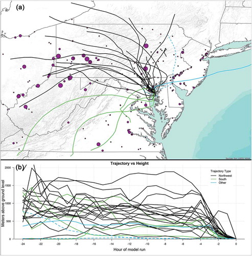
Backward trajectories originating over the HMIPOM at 10m height above the NCB were modeled for 24 hours from the hour of peak ozone on each HMI exceedance day using the Air Resource Laboratory’s (ARL) Hybrid Single Particle Lagrangian Integrated Trajectory (HYSPLIT) model (Rolph, Stein, and Stunder 2017) using the 3 km resolution High Resolution Rapid Refresh (HRRR) meteorological dataset. Consistent with other aloft measurements, air parcels on 17 of 24 (71%) days came from the north and/or northwest, four (17%) came from the south, and the remaining three exceedance days were easterly or localized recirculating air. The veering winds observed between the surface and the 0.5–1.5 km PBL was manifest as a directional inflection or trajectory button-hook as air entered the NCB, particularly evident within the northwest trajectories (Figure 4a). The northwest trajectories entered the NCB and turned as they descended to approach the island from the south explaining the disparity between surface and aloft wind direction. A majority (83%) of exceedance day trajectories showed at least 500 m of subsidence before reaching the surface of the Chesapeake Bay (Figure 4b). Two of the four days not showing at least 500 m subsidence were from coarse NAM 12 km meteorology, which was required on two days due to unavailable HRRR HYSPLIT files.

Figure 4. 24-hour backwards trajectories for all 24 days in which HMI MD8AO exceeded 70 ppbv in an east-west plan view (a) and vertical cross section (b). Black trajectories fell within the north/northwest grouping, green trajectories were within the southerly group and blue fell in neither category but were loosely classified as easterly and/or “anomalous”. The two dashed trajectories used NAM meteorology (12 km). All other trajectories used HRRR meteorology (3 km). Colored circles in (a) showed average daily NOx emissions sized proportionately by magnitude in 2016 from electrical generating units in select states.

High elevation ozone observations

Diurnal mixing of the residual layer played a key role in MD8AO concentrations in Maryland historically (e.g. Aburn et al. 2015; Dreessen, Sullivan, and Delgado 2016; Ryan et al. 1998). A residual layer with low pollutant load will dilute surface layer pollutants via vertical mixing while a residual layer with greater pollutant load may lead to higher MD8AO as mixed pollutants sustain surface concentrations. This study suggests similar reasoning applies to the NCB as well. Ozone monitors at high elevation can serve as a continuous quantitative measure of pollutant load in the nocturnal residual layer. Three sites offer such observations around Maryland: Shenandoah National Park, Virginia (SNP; 38.52° N, −78.43° W; 1070 m above sea level (ASL)), Piney Run, Maryland (39.71° N,-79.01° W; 766 m ASL), and Methodist Hill, Pennsylvania (39.96° N,-77.48° W; 622 m ASL). MD8AO for all days at HMI correlated (r) well with MD8AO at Piney Run (0.51) and SNP (0.47), though saw no correlation with the lowest site, Methodist Hill (0.04). Correlation with elevated ozone samples was intuitive given trajectory subsidence into the NCB from at least 500 m, implying the residual layer likely influenced surface ozone concentrations of the NCB.

Additional elevated measurements were available with vertical profiles provided by ozonesondes launched at Howard University’s Beltsville, Maryland Research Campus (HUBRC; 39.055°N, 76.878°W) co-located with the MDE HU-Beltsville monitor. Between 2016 and 2017, there were 16 days on which ozonesondes were launched while the HMIPOM was deployed. Mean layer concentrations from 0.5– 1.5 km using predawn (1:00– 3:30 am EST) ozonesondes quantified the ozone within the residual layer impacting later-day ozone production. There were 13 pre-dawn ozonesondes launched on a day with a maximum temperature ≥85°F at BWI with mostly sunny conditions. These 13 were split between exceedance (eight) and non-exceedance days (five) at HMI (Figure 5a). The average residual layer concentrations were 45.2 ppbv for non-exceedance days and 52.8 ppbv for exceedance days. The MD8AO difference observed on the surface at HMI between these days was 23 ppbv: 58 ppbv on non-exceedance days, 81 ppbv on exceedance days.

Figure 5. (a) Morning ozonesondes (1:00–3:30 am EST) launched from the Howard University (HU-) Beltsville Campus. Blue represents ozonesondes launched on days with HMI not exceeding 70 ppb. Red represents ozonesondes during days with HMI MD8AO above 70 ppb. Fine lines are individual profiles while the bold lines show the average of the group. The ozonesonde from September 28, 2017, was not included in the non-exceedance day ozonesonde average profile. (b) Hourly ozone concentrations on May 15–18, 2017 observed at the elevated (1070 m) monitor in Shenandoah National Park (SNP) in Virginia. Ozone at the site dropped during the early morning hours on May 18 keeping HMI from exceeding.

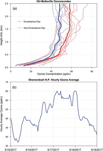
Direct examples of the residual layer influence on HMI were obvious. On May 17, 2017 transported smoky air was associated with peak ozone concentrations of 65 ppbv at SNP as the polluted air arrived in Maryland during the early morning hours (Figure 5b). The SNP observations were corroborated and consistent with a concurrently launched ozonesonde at HUBRC. The MD8AO at HMI on May 17 was 72 ppbv, an exceedance of the NAAQS despite air temperatures reaching only 73°F at HMI. Residual layer ozone concentrations quickly dropped on May 18 (Figure 5b) to reflect cleaner regional background conditions (40–50 ppbv) by midday on May 18. Despite peak MD8AO concentrations reaching 90 ppbv at other monitors in Maryland on May 18, HMI reached only 65 ppbv for its MD8AO, 25 ppbv lower than the highest monitor in Maryland with essentially identical trajectories both days. Similar circumstances existed on September 28, 2017 when a predawn ozonesonde measured residual layer concentrations of 62.3 ppbv yet MD8AO at HMI was 41 ppbv. Again consistent with the ozonesonde, hourly surface ozone at SNP was 64 ppbv from 1–2 am EST. However, concentrations at SNP decreased to 41 ppbv by 9 am EST, influencing the MD8AO that day at HMI in similar behavior to the May 17–18, 2017 case.

The impact of wind direction on HMI ozone

Nine exceedance days in Maryland did not simultaneously support sustained ozone at HMI and elsewhere in the state, providing a unique comparative opportunity (Table 4). Only Hagerstown in western Maryland exceeded on June 15, 2017. However, because Hagerstown was within polluted air along a back-door frontal convergence zone and not within the same post-frontal airmass as HMI, it was not considered further. The remaining eight exceedance days all had supportive meteorological conditions for exceedance days over the NCB but did not result in or sustain ozone in excess of 70 ppbv at the HMI site. Seven of the eight days featured trajectories from the south or southwest. The remaining day was narrowly an exceedance day (MD8AO of 70 ppbv) but had relatively weak 0.5–1.5 km northwest wind speeds and a clear convergence boundary and/or trough axis west of the NCB, some distance from HMI on radar (July 6, 2016; not shown). June 10 and 11, 2017 showcased significantly different ozone spatial patterns seemingly dictated by the wind direction. Hot temperatures and a southwesterly wind at 50 and 500 m on Saturday, June 10 resulted in an exceedance day at Glen Burnie, Aldino, and Fair Hill, but not at HMI. On Sunday, June 11 trajectories switched to the northwest with an ozone exceedance day only at HMI. The eight cases showed that in otherwise ozone conducive conditions, wind speed and direction relative to the NCB land-water interface impacted the amount of ozone at HMI.

Table 4. Conditions during days when Maryland monitors exceeded exclusive of HMI. “DOW” was day of the week, “MD High” was the highest MD8AO concentration seen in Maryland, which can be compared to the MD8AO at Hart-Miller Island “HMI”. “Traj Direct” was the main direction the trajectory approached the greater Baltimore/HMI area from according to HRRR and/or NAM data. The temperature difference was the approximate land-water temperature differential between BWI and the Patapsco Buoy. SNP was utilized as a proxy measurement of the ozone load within the residual layer. Greater concentrations within the residual layer historically have led to greater surface MD8AO.

			MD8AO (ppb)			Traj Direct		Temperature Diff (°F)
DATE	DOW	BWI Tmax	MD High	HMI	SNP	50m	500m	Morning	Afternoon
7/6/2016	Wed	92	74	70	36*	NW	NW	9.1	−11.9
7/16/2016	Sat	92	71	67	47	SW	W	15.3	−8.7
7/25/2016	Mon	100	77	70	43	SW	W	9.5	−14.5
8/31/2016	Wed	91	73	67	49	S	S	18.8	−7.2
5/18/2017	Thu	92	90	65	49	SW	SW	−7.0	−27.1
6/10/2017	Sat	89	73	65	54	SW	SW	15.9	−16.1
6/15/2017	Thu	85	71	51	46	E-SE	E	14.5	−5.5
6/22/2017	Thu	88	71	70	46	S	W	12.4	−7.6
9/25/2017	Mon	89	75	54	53	SE	SE	15.5	−9.5

Notes. *Hours missing during day

Model comparisons

Comparison of surface MD8AO in CMAQ with observations at HMI revealed the NOAA CMAQ had overall root mean square error (RMSE) of 10.3 ppbv and a 4.5 ppbv high bias, representing an 8.1% higher forecast averaged for all days, with a maximum over-prediction of 37 ppbv on July 25, 2016 (e.g., Figure 1) and greatest under-prediction of 22 ppbv on September 23, 2016 (Figure 6). The under-prediction missed an exceedance day while the over-prediction was a false alarm (a situation with predicted values above 70 ppbv and observations at or below 70 ppbv) at HMI, highlighting some model difficulties over water. Of the 21 Maryland ozone monitors in operation over the same period, HMI had the second-highest number of false alarms. The highest false alarm rate occurred at a land/water grid site (Horn Point) far from the Baltimore-Washington DC corridor. The HMI RMSE and bias were not the highest of Maryland sites, but HMI remained in the top half of monitors for bias, and in the top third for RMSE. For all 24 observed exceedance days at HMI, the RMSE of the model was 11.6 ppbv with only 0.8 ppbv bias. Greatest over and under-predictions were both 22 ppbv. While there were only 24 exceedance days observed at HMI, the CMAQ model forecast 52. For these 52 days the CMAQ model had RMSE of 16.2 ppbv and a 12.8 ppbv high bias representing a forecast 15.5% greater than observed. In these circumstances, HMI bias and RMSE were both second only to Horn Point within the Maryland monitoring network.

Figure 6. Scatter plots of Maximum Daily 8-hour Average Ozone (MD8AO) concentration at HMI against CMAQ forecast MD8AO concentration in 2016 and 2017. A least squares line of best fit to the data is shown for each year. The bottom time series showed daily model error (modeled MD8AO minus HMI observation) at HMI over the two-year study period, with 2016 in red, and 2017 in blue. Positive numbers are model over-prediction, negative numbers show under-predictions. Overall the model over predicts at the site.

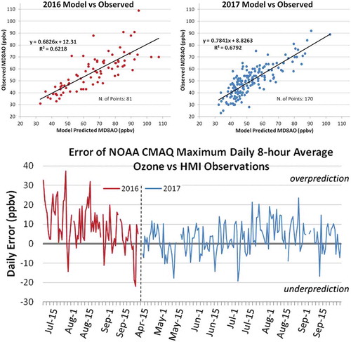
Disparity existed between 2016 and 2017 in the model performance. RMSE and bias were 13.9 ppbv and +8.5 ppbv in 2016, respectively, but only 8.1 ppbv and +2.6 ppbv in 2017. As previously mentioned, 2016 was warmer overall and presented more cases with northwest winds supportive of transport across the land-water interface of the NCB while conditions were ozone supportive. These circumstances partially explained the disparity in forecast accuracy between the years. The better forecasted, larger 2017 dataset likely also bettered the overall model performance statistics due to the shorter but more meteorologically supportive 2016 dataset. However, the forecast model upgrade in 2017 adds uncertainty.

Emissions

EGUs and Point Sources

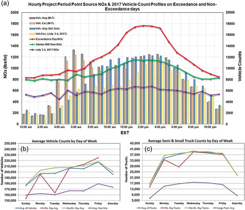
There were several significant NOx point sources in the southern Baltimore region (cross-hatched area in Figure 1) including several EGUs and municipal waste combustor (MWC). These five facilities reported daily aggregate NOx emissions in a range of 2.3–22.0 tons during the two seasons of study within a relatively dense spatial area. Among the 24 exceedance days at HMI, there were two when these five Baltimore point sources had emissions 50% lower, ~2 standard deviations, than the exceedance day group mean (purple line, Figure 7a). Due to their distinctive NOx profile and the coincidental timing with a holiday, these July 3 and 4, 2017 exceedance profiles were treated separately. The daily average difference between the remaining 22 exceedance and 100 non-exceedance days when the high temperature at BWI was at least 85°F was ~2 tons with 0.98 tons of the difference occurring between 9 am and 3 pm EST. Furthermore, there were 23 days which had northwesterly trajectories not impacted by clouds or storms, and which the high temperature at BWI was at least 85°F but were not exceedance days at HMI. Both daily and midday (9 am – 3 pm EST) emissions were statistically different between this non-exceedance subgroup (green line, Figure 7a) and the HMI exceedance day group (red line, Figure 7a) with a daily NOx emissions difference of approximately 2.8 daily tons, 53% (1.5 tons) of which occurred 9 am-3 pm EST. Thus, greater aggregated southern Baltimore region point source NOx emissions during northwest flow were coincidental with greater ozone at HMI.

Figure 7. (a) Average aggregate diurnal hourly NOx output from Baltimore area point sources (lines) during HMI exceedance days (red), minus two exceedance days with uncharacteristically low emissions during a holiday period (purple) compared to the average NOx profile during warm days with northwest flow (green). The number of cars on I-95 counted at the MDE Near-Road Site located between Baltimore and Washington DC (bars) for weekday and weekend/holiday, average and exceedance day subgroups was also provided. “Exc.” indicates an exceedance day group and “Avg” indicates average of all car count days. (b) Graph of average vehicle counts by day of the week for entire 2017 May-September (“average”, blue), day of week average on exceedance days (“Exc. Average”, red), warm, non-exceedance days (“Non-Exc. Average”, green) and day of the week average for passenger cars/pickup trucks only, over the entire May-September 2017 period (“Avg Cars Only”, purple). (c) Similar to graph in b, except for combination truck (“semi-truck”) day of the week averages over the entire period (blue), exceedance days (red), warm non-exceedance days (green) and a separately counted category of smaller, non-passenger truck vehicles. No exceedance day occurred on a Saturday in 2017.

Mobile

A Wavetronix SmartSensor HD traffic sensor at the MDE near-road site adjacent to Interstate-95 between Baltimore and Washington DC (Figure 1) used K-band radio frequency to track vehicle counts, speed, and vehicle type in high temporal frequency since 2017. Regional vehicular volume may be represented by these vehicle counts. To investigate possible connections between mobile emissions and ozone concentrations, vehicle counts from May through September 2017 provided a quantitative comparison between exceedance and non-exceedance days as well as average conditions within the second season of the study. Vehicle statistics included all mobile units, from small cars to multi-unit trucks.

A large disparity in vehicle counts existed between weekday (Monday – Friday) and weekend (Saturday, Sunday)/holidays (July 4) requiring treatment of these two groups separately (Figure 7a). An insignificant 1.1% decrease in total cars existed on weekday exceedance day mornings compared to the average of all other weekday mornings (4 am-9 am EST) and a 3.7% significant decrease compared with other warm non-exceedance days. Total vehicles counted, of which passenger cars and trucks comprised the overwhelming majority, was lowest on Sunday and greatest on Friday, with a general increase exhibited through the week (Figure 7b). Large combination (“semi”) trucks and smaller classified trucks (e.g., dump trucks) comprised much of the difference between passenger cars and the total vehicle count. Both truck categories had a peak in activity on Wednesday with counts on Saturday and Sunday nearly one-third of the peak (Figure 7c). Like total vehicles, little difference existed between average conditions and exceedance day truck counts. The small truck category had counts below the seasonal daily average during high ozone days.

Marine

Counts of commercial marine vehicles (i.e., cargo ships) entering the Port of Baltimore were provided by the Maryland Port Authority. No correlation was found between ship counts and MD8AO concentrations at HMI. However, neither ship type nor information regarding length in port was analyzed. Additionally, no observational data on small pleasure craft was known to the authors. Pleasure craft was hypothesized to be a pertinent issue, as exceedance days occurred at HMI on July 3 and 4, 2017, during a significant drop in vehicular counts (117,107 total vehicles on July 4; seasonal daily weekday average was ~205,000 vehicles) and EGU emissions (Figure 7a). Hard data on operating pleasure craft was not collected, but the Department of Natural Resource police report the Independence Day holiday drastically increased the number of recreational boaters in the NCB (personal communication). Pleasure craft emissions have been implicated previously (Henry 2013). It was therefore plausible the HMI exceedance days during the Independence Day holiday were due to pleasure craft, but additional data and investigation are needed.

Discussion

Analysis of exceedance days at HMI exhibited three distinct features: 1) northwest flow in the PBL flowing past Baltimore toward the NCB, 2) descending air toward the surface of the NCB south of HMI, 3) southerly surface winds at HMI coincident with the highest ozone concentrations and/or the onset of increasing ozone concentrations. Northwest flow by itself was insufficient but needed augmented ozone or precursor load within the regional PBL or enhanced local emissions near Baltimore to exceed the ozone NAAQS over the NCB. Mountain-top and balloon-borne measurements observed greater ozone aloft on days with higher ozone concentrations at HMI, consistent with the descending trajectories transporting enhanced ozone from at least the 0.5–1.5 km layer to the surface. Descending air in the bay breeze circulation then caused mass adjustments that induced southerly surface winds at HMI, associating them with increased ozone as NCB land-water thermal circulations matured. This primary exceedance day model may be influenced by the evolution of the bay breeze circulation, which itself was impacted by several factors including the geography of the coastline and the synoptic wind, consistent with Miller et al. (2003). The vertical exchange within this primary exceedance day archetype indicated that the NCB would be directly impacted by both local emissions and long-range transport.

Land-sea breeze three-dimensional dynamics partially explains daily and intra-day ozone variability in the NCB. As the orthogonal component of the wind to the coastline decreases, marine air in the landward moving surface branch of the bay breeze circulation may progress further in-land, while the elevated waterward branch is simultaneously weakened and displaced landward removing the transport of land-based emissions from the center of the NCB. Weaker northwest flow on July 6, 2016 decreased precursor transport over the NCB, removing them from subsidence over the central NCB, keeping HMI from exceeding. A wind from the southwest (with nominal orthogonal wind component) would cause a NCB coast-parallel elevated return branch of the bay breeze. In such a case, the bay breeze circulation becomes corkscrew-like (Miller et al. 2003; Steele et al. 2013) along the coast south of Baltimore and local emissions from Baltimore never move over the NCB. Oscillations in the wind could therefore produce oscillations in the chemical fields.

Furthermore, marine meteorology may explain the unique diel behavior of ozone over water. Ozone was more than 9 ppbv higher in the afternoon on average at HMI than nearby land sites during exceedance days. The morning ozone development also was consistently delayed. Stagnation and aggregation of precursors overnight due to a weakening or reversal of the bay breeze may predispose the NCB to high ozone due to its spatial proximity to sources in Baltimore. While a likely occurring scenario, ozone remained as much as 12 ppbv higher overnight over the water, indicating a lack of titration and that fresh emissions were unlikely reaching the water surface near HMI. Lacking NOx titration and ozone deposition over water as compared to land sites have been well-established explanations for higher ozone over water (e.g., Goldberg et al. 2014), yet exceedance day morning profiles were similar to other average days, suggesting little change between days prior to sunrise. Therefore, while a previous day’s ozone and chemical composition may persist over the water overnight and into the early morning, the surface air appeared to be separate from air above or adjacent to it, including the titrating effects from stagnating air and aggregating precursors over land.

Persistence of the surface air over the water independent from that over land could explain the delay in ozone development. Assuming that nominal ozone titration over water indicates no new emissions or addition of precursors, the morning delay in ozone development could have resulted from the delayed introduction of precursors held above the surface layer. Another plausible explanation may be a delay in thermal decoupling of reservoir NOx species due to delayed air temperature increases over the water. However, it is interesting that the delay in surface ozone development at HMI coincides well with the typical time of bay breeze initiation, making the prior explanation more plausible.

In the delayed recoupling of the NCB surface layer scenario just discussed, northwest winds in the PBL would transport local emissions and/or polluted residual layers toward the NCB where subsidence within a mature bay breeze circulation would introduce pollutants into the NCB surface layer. In this scenario, release height, transport height, and proximity to water become fundamentally important. Abundant thermal mixing on land that disperses NOx plumes does not exist within the stratified, subsiding air into NCB. Hindered dispersion over the NCB would sustain higher NOx concentrations, particularly within locally emitted plumes immediately adjacent to the NCB. The greater localized NOx concentration results in enhanced ozone in the NOx limited air. It is assumed the NCB water temperature does not prohibitively stabilize the marine air and prevent downward transport to the surface layer and may explain why exceedance days favored warmer water. The decoupling of the near-surface with that above could also explain why, in certain circumstances, Bay air was cleaner compared to other polluted sites in the region as occasionally noted by air quality forecasters: transported pollutants never entered the marine surface layer but remained vertically adjacent to it. A shallow surface layer independent of the air vertically adjacent to it could also suggest an explanation to some of the HMI-only exceedance days. For instance, surface-emitting pleasure craft would support high ozone only over the NCB.

Increased performance of the NOAA CMAQ model was noted between 2016 and 2017. While mean weather between the seasons accounts for some model performance differences, improvements in VOC reactions and in the activation of NTR-cycling for ozone production was believed to be partially responsible for lower forecast error at HMI 2017. This was a potentially significant finding if certain NOx reservoir species (such as NTR or PAN) explained the morning delay in ozone production at HMI. PAN, the most abundant species of Acyl Peroxy Nitrate, experiences prolonged life-time in cooler marine PBLs than in adjacent land PBLs as delayed heating over the water reduces thermal decoupling (Seinfeld and Pandis 1998), delaying photochemical production of ozone upon sunrise. In such a case, the marine air shed acts as a reservoir of reservoirs of the previous day’s pollution. Note the surface chemical reservoir here was different than the elevated residual layer described earlier and the reservoir described in He et al. (2014). While a vertical exchange mechanism discussed previously is the favored explanation for the delay, it is still reasonable to assume the surface layer may act as a reservoir and may account for the delayed ozone onset in some cases. Future speciated observations will answer these questions.

Finally, exceedance days at HMI had increasing afternoon ozone concentrations relative to declining concentrations on non-exceedance days. Additional ozone precursors on exceedance day afternoons likely explain this finding. In the NOx limited regime (Goldberg et al. 2014), decreased NOx dispersion in the stratified marine air and/or increased NOx emissions from southern Baltimore would increase ozone concentrations within the marine layer relative to land sites. The bay breeze circulation typically reaches maturity during the afternoon and could deliver ozone laden air to the NCB surface. Relatively minor enhanced NOx emissions and local transport during critical hours of the afternoon could be sufficient to sustain ozone for the required 8 hours for an exceedance. This would be particularly true in the non-dispersed, NOx limited air of the NCB if emitted above the surface along the coast. Slight changes in EGU profiles would fulfill this requirement.

The NOAA CMAQ model captured high ozone over the water during observed events at HMI, showing the model adequately portrays ozone development over water. The primary issues were the high bias and proclivity to false alarm. This may be due to several reasons. If the emissions are not adequately transported over the water or quantified from the urban area, ozone may appear too aggressive. A 12 km grid spacing is too coarse to adequately resolve the fine-scale meteorology and transport occurring. Loughner et al. (2011) showed finer resolution better resolves the bay breeze. Consistent with Loughner et al., MDE forecasters have noted 12 km operational meteorological models do not resolve the bay breeze as well as finer-scale models. Thus, it may be that the coarse resolution improperly resolves the chemical transport within the operational model. Consequently, an over-estimation of nearby land sites is apparent. For instance, even accurately forecast ozone over water in a situation similar to Figure 1 will cause nearby coastal sites to be overestimated due to the inability at 12 km resolution to adequately resolve ozone gradients of tens of ppbv over less than a kilometer. While the model more closely matches reality when observed ozone is above 70 ppbv over water, a high bias over water for all days inadequately portrays coastal sites in SIP type seasonal averaging. This is not to discount the NOAA CMAQ, but illustrate the shortcomings of a 12 km model for state compliance modeling. Indeed, in a forecasting context, situational awareness and knowledge of the conceptual model of exceedances over the NCB makes the 12 km resolution NOAA CMAQ model an effective and irreplaceable decision support tool.

Varying wind direction presented southern Baltimore as a pivot point during ozone exceedance days. For example, southwest winds on June 10, 2017 were associated with exceeding ozone monitors northeast of southern Baltimore (Figure 1 cross-hatched area) but outside of the NCB. Then northwest winds on June 11, 2017 were associated with an ozone exceedance day nowhere but at HMI. A significant number of NOx point sources operated across southern Baltimore, with EGUs and a MWC comprising the majority of emissions mass. Statistical tests suggested the amount and timing of NOx emissions from some of the largest point sources from this area was the primary difference between exceedance and non-exceedance days at HMI. Additional afternoon NOx likely sustained the afternoon ozone concentrations observed on the diurnal profiles during exceedance days. The initial assessment implicated hourly NOx emission mass from local point sources under favorable winds as a primary driving factor for sustained ozone concentrations greater than 70 ppbv over the NCB in this study. Though evidence exists, it remains possible these connections are circumstantial. Other non-EGU point sources exist in this southern Baltimore region but emissions are reported on an annual basis. Little is known about the daily variability of these sources. Future satellite retrievals will be useful in that regard. While overall a single large facility may inexorably cause an exceedance day, this study suggests aggregate NOx is key. This study also strongly suggests that key components to the NCB ozone issue lie in the chemistry occurring immediately over and downwind of southern Baltimore.

The mobile sector contributes to ozone at HMI, but the lack of variability in vehicle counts and discrimination between exceedance and non-exceedance days suggests vehicles, under normal driving conditions, are not sufficient for high ozone at the HMI site. Greater ozone during the work week than on the weekend was assumed to be a consequence of commuting vehicles since their numbers have significant disparity between work week and weekend. However, no statistical significance was found. The relatively consistent daily number of work week vehicles (9.3% change from Monday to Friday for the 2017 period) unlikely solely explained ozone variability at HMI. There was some indication that truck traffic influenced the weekly cycle, but it too was not significant. The analysis suggested vehicles provide an accumulated ozone background. This study did not look at vehicle speed or driving conditions. It is also possible the HCNR site did not capture vehicle count variability where needed, such as near Baltimore industry.

Conclusions

This study produced the first multi-season ozone record over the NCB documenting the frequency of, meteorological conditions conducive to, transport patterns on, model verification of, and representative emissions during exceedance days at HMI. In total, 24 exceedance days of the EPA 70 ppbv NAAQS were observed at HMI. MD8AO concentrations at HMI were most frequently the highest in the state but not exclusively so. These observations were consistent with previous studies that reported higher ozone over the NCB than nearby coastal sites but documented specific conditions that commonly led to ozone in excess of 70 ppbv NAAQS over the NCB water.

A button-hook transport pattern accounted for at least 71% of exceedance days over the NCB. HYSPLIT trajectory modeling demonstrated an archetype exceedance day with northwesterly transport over the greater Baltimore area, after which trajectories descended toward the NCB surface. During the descent, these trajectories turned to be from the south, creating a button-hook pattern and southerly surface winds at HMI. Surface ozone at HMI exhibited ozone increases primarily during southerly winds, sometimes with changes of over 10 ppbv in 10 minutes. Most trajectories impacting HMI descended over 500 m and passed by abundant precursor sources of southern Baltimore. Thus the transport pattern linked the southerly surface winds observed during high ozone at HMI with northwest winds concurrently observed in the 0.5–1.5km layer. Consequently, locally sourced or long-distance transport of ozone and ozone precursors may be delivered to the NCB from in this primary exceedance archetype. This air may continue to coastal sites, creating ozone laden bay breezes at Maryland monitors. As such, historically critical bay breeze ozone events at Edgewood, Maryland were likely manifestations of long-range transport exacerbated by the Baltimore plume.

Distinguishing between local and long-distance transport will be vital to the state to ensure that ozone exceedance days continue to decrease. In the contemporary NOx limited regime, increased NOx sensitivity means local emissions play an increasingly important role in driving ozone concentrations and distributions in the Maryland region. Locally heightened NOx emissions were evident on exceedance days as evidence pointed to Baltimore area stationary sources as potential contributors necessary to sustain ozone concentrations on exceedance days within the NCB on 22 of 24 days. Evidence of mobile source contribution existed as well but was not statistically significant. However, exceedance days were also observed at HMI with low emissions from point and mobile sources, suggesting potential influence from pleasure boats on these holiday exceedances. Ultimately, ozone over the NCB depended on the morphology of the bay breeze circulation, ozone precursor release, and horizontal and vertical transport across the NCB land-water interface. While southern Baltimore was identified as a culpable source region of precursors, observations of VOCs and NOy/NOx were needed to further apportion attribution by sector.

For the first time, a multi-season verification of a CMAQ model over the water was possible. A high bias was noted for the operational 12 km NOAA CMAQ model. Though 24 exceedance days were observed, 52 such days were forecast by the NOAA CMAQ, collectively 15.5% higher than that observed over the water during these days. The model did better when exceedance days were observed at HMI but same-day MD8AO was 8.1% high over all days for both seasons of the study. The NOAA CMAQ was non-regulatory, but matches the resolution mandated by the EPA for state modeling. The over-prediction noted in this operational model may represent over-prediction to be found within state and federal SIP modeling framework with ramifications which may potentially create flawed control strategies. The coarse resolution in the model does not capture the sharp gradients noted in the study, showing that even in circumstances of high ozone over the NCB, the smearing across grid cells may not appropriately account for the heterogeneity found along the coast line, disproportionately allocating ozone to coastal monitors. Additionally, if models cannot adequately capture the vertical processes or resolve the sharp gradients found in this study, a model should neither be expected to adequately characterize source attribution at coastal sites.

This study serves as guidance to the OWLETS-2 campaign and other future studies of ozone development over the NCB. The OWLETS-2 follow-up campaign will support high-resolution observations and modeling. Study of the vertical structure of ozone and wind over the Bay is also paramount to fully understand the exchange occurring, given the vertical transport observed at HMI in this study. Continuous vertical measurements of ozone and meteorology are paramount to confirm this vertical transport exchange. Future work should focus on specific observations which will best support policy needs at the state level, such as differentiating and quantifying the contribution between local and regional sources. If possible, measuring pollutant species and VOCs which can serve as tracers to source sector and pollutant age at HMI would be ideal. Retrospective analysis using the latest policy driven version of CMAQ, meteorology, and emissions will be utilized.

Acknowledgments

The authors extend sincere gratitude to the Maryland Port Authority and Maryland Environmental Services for their invaluable assistance and cooperation in facilitating transport to and from Hart-Miller Island for the duration of the project. The authors also thank reviewers for their valuable input to improve this work. This project was made possible through the work of the Maryland Department of the Environment (MDE) with equipment funded through an EPA state and tribal work grant. Views expressed in this paper are those of the authors and do not necessarily reflect those of MDE or NOAA.

Disclosure statement

No potential conflict of interest was reported by the authors.

Additional information

Notes on contributors

Joel Dreessen

Joel Dreessen is senior meteorologist at the Maryland Department of the Environment within the air monitoring program in Baltimore, MD.

Daniel Orozco

Daniel Orozco is an air quality researcher at the Maryland Department of the Environment within the air monitoring program in Baltimore, MD.

James Boyle

James Boyle is a meteorologist at the Maryland Department of the Environment within the air monitoring program in Baltimore, MD.

Jay Szymborski

Jay Szymborski is a lead for technical support and special projects with the Maryland Department of the Environment within the air monitoring program in Baltimore, MD.

Pius Lee

Pius Lee is a physical scientist in NOAA Air Resources Laboratory responsible for leading research for the US National Air Quality Forecasting Capability.

Adrian Flores

Adrian Flores is a research technician at the Howard University Beltsville Campus conducting atmospheric research for NOAA Cooperative Science Center in Atmospheric Sciences and Meteorology (NCAS-M) and GCOS Reference Upper-Air Network (GRUAN).

Ricardo K. Sakai

Ricardo K. Sakai is the senior research scientist at Howard University, Beltsville Campus.

References

- Aburn, G., R. R. Dickerson, J. C. Hains, D. King, R. Salawitch, T. Canty, X. Ren, A. M. Thompson, and M. Woodman. 2015. Ground level ozone: A path forward for the eastern United States. E.M., May, 18–24. http://pubs.awma.org/flip/EM-May-2015/aburn.pdf.
- Biggs, W. G., and M. E. Graves. 1962. A lake breeze index. J. Appl. Meteorol. 1 (4):474–80. doi:10.1175/1520-0450(1962)001<0474:ALBI>2.0.CO;2.
- Bloomer, B. J., Y. V. Konstantin, and R. R. Dickerson. 2010. Changes in seasonal and diurnal cycles of ozone and temperature in the eastern US. Atmos. Environ. 44 (21–22):2543–51. doi:10.1016/j.atmosenv.2010.04.031.
- Crossett, K., B. Ache, P. Pacheco, and K. Haber. 2013. National coastal population report, population trends from 1970 to 2020. NOAA State of the Coast Report Series, US Department of Commerce, Washington. Accessed May 15, 2019. https://aamboceanservice.blob.core.windows.net/oceanservice-prod/facts/coastal-population-report.pdf.
- Dreessen, J., J. Sullivan, and R. Delgado. 2016. Observations and impacts of transported Canadian wildfire smoke on ozone and aerosol air quality in the Maryland region on June 9 –12,2015. J. Air Waste Manage. Assoc. 66 (9):842–62. doi:10.1080/10962247.2016.1161674.
- Frysinger, J. R., B. L. Lindner, and S. L. Brueske. 2003. A statistical sea-breeze prediction algorithm for Charleston, South Carolina. Weather Forecast. 18 (4):614–25. doi:10.1175/1520-0434(2003)018<0614:ASSPAF>2.0.CO;2.
- Gégo, E., P. S. Porter, A. Gilliland, and S. T. Rao. 2007. Observation-based assessment of the impact of nitrogen oxides emissions reductions on ozone air quality over the eastern United States. J. Appl. Meteorol. Climatol. 46 (7):994–1008. doi:10.1175/JAM2523.1.
- Goldberg, D. L., C. P. Loughner, M. Tzortziou, J. W. Stehr, K. E. Pickering, L. T. Marufu, and R. R. Dickerson. 2014. Higher surface ozone concentrations over the Chesapeake Bay than over the adjacent land: Observations and models from the DISCOVER-AQ and CBODAQ campaigns. Atmos. Environ. 84:9–19. doi:10.1016/j.atmosenv.2013.11.008.
- He, H., C. P. Loughner, J. W. Stehr, H. L. Arkinson, L. C. Brent, M. B. Follette-Cook, M. A. Tzortziou, K. E. Pickering, A. M. Thompson, D. K. Martins, et al. 2014. An elevated reservoir of air pollutants over the Mid-Atlantic States during the 2011 DISCOVER-AQ campaign: Airborne measurements and numerical simulations. Atmos. Environ. 85:18–30. doi:10.1016/j.atmosenv.2013.11.039.
- Henry, R. F. 2013. Weekday/weekend differences in gasoline related hydrocarbons at coastal PAMS sites due to recreational boating. Atmos. Environ. 75:58–65. doi:10.1016/j.atmosenv.2013.03.053.
- Janjić, Z., and R. Gall. 2012. Scientific documentation of the NCEP nonhydrostatic multiscale model on B grid (NMMB). Part 1 dynamics. NCAR Technical Note NCAR/TN-489+STR: 80.
- Laird, N. F., D. A. Kristovich, X. Liang, R. W. Arritt, and K. Labas. 2001. Lake Michigan lake breezes: Climatology, local forcing, and synoptic environment. J. Appl. Meteorol. 40 (3):409–24. doi:10.1175/1520-0450(2001)040<0409:LMLBCL>2.0.CO;2.
- Landry, L. 2011. The influence of the chesapeake bay breeze on maryland air quality. Paper presented at the annual MARAMA Data Analysis Workshop, College Park, MD, January 19–20. http://www.marama.org/presentations/2011_DataAnalysis/LLandry_MARAMA-20110120.pdf.
- Lee, P., J. McQueen, I. Stajner, J. Huang, L. Pan, D. Tong, H. Kim, Y. Tang, S. Kondragunta, M. Ruminski, et al. 2017. NAQFC developmental forecast guidance for fine particulate matter (PM2. 5). Weather Forecast. 32 (1):343–60. doi:10.1175/WAF-D-15-0163.1.
- Lennartson, G. J., and M. D. Schwartz. 2002. The lake breeze–Ground‐level ozone connection in eastern Wisconsin: A climatological perspective. Int. J. Climatol. 22 (11):1347–64. doi:10.1002/joc.802.
- Loughner, C. P., D. J. Allen, K. E. Pickering, D. L. Zhang, Y. X. Shou, and R. R. Dickerson. 2011. Impact of fair-weather cumulus clouds and the Chesapeake Bay breeze on pollutant transport and transformation. Atmos. Environ. 45 (24):4060–72. doi:10.1016/j.atmosenv.2011.04.003.
- Loughner, C. P., M. Tzortziou, M. Follette-Cook, K. E. Pickering, D. Goldberg, C. Satam, A. Weinheimer, J. H. Crawford, D. J. Knapp, D. D. Montzka, et al. 2014. Impact of bay-breeze circulations on surface air quality and boundary layer export. J. Appl. Meteorol. Climatol. 53 (7):1697–713. doi:10.1175/JAMC-D-13-0323.1.
- Lyons, W. A. 1972. The climatology and prediction of the Chicago lake breeze. J. Appl. Meteorol. 11 (8):1259–70. doi:10.1175/1520-0450(1972)011<1259:TCAPOT>2.0.CO;2.
- Martins, D. K., R. M. Stauffer, A. M. Thompson, T. N. Knepp, and M. Pippin. 2012. Surface ozone at a coastal suburban site in 2009 and 2010: Relationships to chemical and meteorological processes. J. Geophys. Res. 117 (D05306). doi: 10.1029/2011JD016828.
- Miller, S. T. K., and B. D. Keim. 2003. Synoptic-scale controls on the sea breeze of the central New England coast. Weather Forecast. 18 (2):236–48. doi:10.1175/1520-0434(2003)018<0236:SCOTSB>2.0.CO;2.
- Miller, S. T. K., B. D. Keim, R. W. Talbot, and H. Mao. 2003. Sea breeze: Structure, forecasting, and impacts. Rev. Geophys. 41 (3). doi: 10.1029/2003RG000124.
- Mitchell, K. E., D. Lohmann, P. R. Houser, E. F. Wood, J. C. Schaake, A. Robock, B. A. Cosgrove, J. Sheffield, Q. Duan, L. Luo, et al. 2004. The multi-institution North American Land Data Assimilation System (NLDAS): Utilizing multiple GCIP products and partners on a continental distributed hydrological modeling system. J. Geophys. Res. 109:D07S90. doi:10.1029/2003JD003823.
- Pleim, J. E. 2007. A combined local and nonlocal closure model for the atmospheric boundary layer. Part I: Model description and testing. J. Appl. Meteorol. Climatol. 46 (9):1383–95. doi:10.1175/JAM2539.1.
- Porson, A., D. G. Steyn, and G. Schayes. 2007. Formulation of an index for sea breezes in opposing winds. J. Appl. Meteorol. Climatol. 46 (8):1257–63. doi:10.1175/JAM2525.1.
- Rasmussen, D. J., A. M. Fiore, V. Naik, L. W. Horowitz, S. J. McGinnis, and M. G. Schultz. 2012. Surface ozone-temperature relationships in the eastern US: A monthly climatology for evaluating chemistry-climate models. Atmos. Environ. 47:142–53. doi:10.1016/j.atmosenv.2011.11.021.
- Ring, A. M., T. P. Canty, D. C. Anderson, T. P. Vinciguerra, H. He, D. L. Goldberg, S. H. Ehrman, R. R. Dickerson, and R. J. Salawitch. 2018. Evaluating commercial marine emissions and their role in air quality policy using observations and the CMAQ model. Atmos. Environ. 173:96–107. doi:10.1016/j.atmosenv.2017.10.037.
- Rolph, G., A. Stein, and B. Stunder. 2017. Real-time environmental applications and display system: READY. Environ. Model. Softw. 95:210–28. doi:10.1016/j.envsoft.2017.06.025.
- Ryan, W. F., B. G. Doddridge, R. R. Dickerson, R. M. Morales, K. A. Hallock, P. T. Roberts, D. L. Blumenthal, J. A. Anderson, and K. L. Civerolo. 1998. Pollutant transport during a regional O3 episode in the mid-Atlantic states. J. Air Waste Manage. Assoc. 48 (9):786–97. doi:10.1080/10473289.1998.10463737.
- Sarwar, G., J. Godowitch, B. H. Henderson, K. Fahey, G. Pouliot, W. T. Hutzell, R. Mathur, D. Kang, W. S. Goliff, and W. R. Stockwell. 2013. A comparison of atmospheric composition using the carbon bond and regional atmospheric chemistry mechanisms. Atmospheric Chem. Phys. 13 (19):9695–712. doi:10.5194/acp-13-9695-2013.
- Schwede, D. 2014. Improvements to the characterization of organic nitrogen chemistry and deposition in CMAQ. Paper presented at the Community Modeling and Analysis System (CMAS) conference, Chapel Hill, October 27. https://www.cmascenter.org/conference//2014/slides/donna_schwede_improvements_treatment_2014.pptx.
- Seinfeld, J. H., and S. N. Pandis. 1998. Atmospheric chemistry and physics: From air pollution to climate change, 205–06. New York, NY: John Wiley & Sons. doi:10.1063/1.882420.
- Sikora, T. D., G. S. Young, and M. J. Bettwy. 2010. Analysis of the western shore Chesapeake Bay bay-breeze. Paper presented at the 17th Conference on Air Sea Interaction, September 28. https://ams.confex.com/ams/17Air17Sat9Coas/techprogram/paper_173944.htm.
- Stauffer, R. M., A. M. Thompson, D. K. Martins, R. D. Clark, D. L. Goldberg, C. P. Loughner, R. Delgado, R. R. Dickerson, J. W. Stehr, and M. A. Tzortziou. 2015. Bay breeze influence on surface ozone at Edgewood, MD during July 2011. J. Atmos. Chem. 72 (3–4):335–53. doi:10.1007/s10874-012-9241-6.
- Steele, C. J., S. R. Dorling, R. Von Glasow, and J. Bacon. 2013. Idealized WRF model sensitivity simulations of sea breeze types and their effects on offshore windfields. Atmospheric Chem. Phys. 13 (1):443. doi:10.5194/acp-13-443-2013.
- Vinciguerra, T., E. Bull, T. P. Canty, H. He, E. Zalewsky, M. Woodman, G. Aburn, S. Ehrman, and R. R. Dickerson. 2017. Expected ozone benefits of reducing nitrogen oxide (NOx) emissions from coal-fired electricity generating units in the eastern United States. J. Air Waste Manage. Assoc. 67 (3):279–91. doi:10.1080/10962247.2016.1230564.
- Wu, W. S., R. J. Purser, and D. F. Parrish. 2002. Three-dimensional variational analysis with spatially inhomogeneous covariances. Mon. Weather Rev. 130 (12):2905–16. doi:10.1175/1520-0493(2002)130<2905:TDVAWS>2.0.CO;2.
- Zhang, D., Y. Shou, R. R. Dickerson, and F. Chen. 2011. Impact of upstream urbanization on the urban heat island effects along the Washington–Baltimore corridor. J. Appl. Meteorol. Climatol. 50 (10):2012–29. doi:10.1175/JAMC-D-10-05008.1.