Comparisons of forward-in-time and backward-in-time Lagrangian stochastic dispersion models for micro-scale atmospheric dispersion

ABSTRACT

Lagrangian stochastic dispersion models are sometimes run in backward mode to estimate air emissions from different types of sources including area sources. The forward-in-time and backward-in-time Lagrangian stochastic (fLS and bLS) dispersion models may not result in the same estimates. The two models were compared under different atmospheric conditions in micro-scale applications. They are equivalent in a steady-state and horizontally homogeneous atmosphere in many features including estimating concentration at a point, using surface receptor, and prerunning the models. Although bLS shows better computational efficiency, it has a larger uncertainty in results due to the use of surface receptors. In a non-steady-state wind field, the two models show opposite transition trends when the wind fields experience a step change. Under sinusoidal-varying winds, the two models show different shapes of the predicated concentration curves. The normalized differences of the mean concentrations mainly increase with the receptor height when the source-receptor distance is fixed. A controlled methane release experiment was conducted to investigate the behaviors of the two models driven by real wind fields. The correlation coefficient between model-predicted concentrations is 0.95. The model-predicted (forward model) and measured concentrations show similar trend with a correlation coefficient of 0.70. The bLS model estimates larger peak concentrations than that fLS model under the same emission rate. The best-fitted results of the fLS and bLS models give recovery ratios of 1.1558 and 0.9675, respectively, which are better than that using a constant 15-min averaged wind (0.7922).

Implications: There are large uncertainties and difficulties in quantification of fugitive air emissions from area sources such as landfills, agriculture, and industry sections. Lagrangian stochastic dispersion model is a versatile tool for these applications with the capability of near-field description and good efficiency. Backward models are usually used to estimate emission rates from area sources due to high computing efficiencies. But they may not result in the same estimate as the forward models due to factors involving model realization and input parameters. It is necessary to investigate the discrepancies to select the best model with minimal uncertainty in the results.

Introduction

Lagrangian stochastic (LS) dispersion model is a versatile tool in modeling diffusion of passive tracers in the turbulent atmospheric boundary layer. It is simple in concept by mimicking particle motion and treating turbulent dispersion as a stochastic process (Stohl et al. 2005). It has advantages of correctly describing the mean concentration field even in the near field from the sources and rationally incorporating all available statistical information about the wind velocity field (Thomson and Wilson 2012). Unlike Eulerian models which are based on grids that are fixed in space, LS models calculate the random path of each particle and update the path at every time step. They are independent of a computational grid and have an infinitesimally high resolution (Stohl et al. 2005). LS models are presently used to treat atmospheric transport and dispersion problems from microscale to global scale (Hegarty et al. 2013; Lin, Brunner, and Gerbig 2011).

LS dispersion models can run in backward-in-time or forward-in-time modes (Flesch, Wilson, and Yee 1995; Seibert and Frank 2004). In forward-in-time LS (fLS) model, particles are released at the source and travel to the receptor location. While in backward-in-time LS (bLS) model, particles are released at the receptor location and travel backward-in-time to the source location. Forward models are usually used to simulate the dispersion of tracers from their sources, while backward models are used in inverse-dispersion technique to determine emission rates from known sources (Stohl et al. 2005), or in the source term estimation (STE) methods to estimate parameters of unknown sources (locations and strengths) (Bieringer et al. 2017). There are several advantages to run the model in backward mode (Eckhardt et al. 2017): (1) It could estimate the concentration at a point without assuming horizontal homogeneity of the flow (Schmid 2002); (2) BLS models show good computational efficiency when the receptor number is less than the source number. Due to these advantages, bLS models were commonly used to estimate ground-air exchange, especially to quantify the emission rate from area sources like landfills, animal feedlots, waste lagoons, etc. (Flesch et al. 2016; Goodrick et al. 2013; Harper et al. 2009; McGinn et al. 2007; Riddick et al. 2016; Wilson, Flesch, and Harper 2001). In the STE applications, the dispersion models need to be combined with estimation algorithm (e.g., optimization or probabilistic approaches) to find the best solution. In the applications of emission quantification, the location and size of the source are usually known, in which case a unique solution can be derived without using estimation algorithm.

Theoretically, the backward and the forward models should result in identical estimates (Batchelder 2006; Kljn et al. 2004). The equivalence between them was proven (Flesch, Wilson, and Yee 1995; Gifford 1959). However, initial comparison studies found that discrepancies may exist due to factors in three categories: the stochastic nature of the models, model realization (e.g., surface reflection scheme, parameterization schemes), and input parameters (e.g., wind fields, source-receptor configurations) (Cai et al. 2008; Hegarty et al. 2013; Kljn et al. 2004; Seibert and Frank 2004). Kljn et al. (2004) compared the concentration footprints predicted by fLS and bLS models in a wind-tunnel test using the same model core. They found good correspondence between these two approaches at low measurement heights (i.e., the receptor near the surface), but significant differences were incurred for measurements higher above the surface (i.e., aloft receptor). They also found differences between peak locations of the footprints for any of the measurement heights. Seibert and Frank (2004) compared the fLS and bLS models in several different tests. They showed the equivalence between forward and backward calculations in simple tests, but different results were obtained when applying them to calculate the concentration of Cs-137 at Stockholm that was emitted from the Chernobyl area. An interesting result is that the forward simulation performs worse according to the calculated correlation coefficient, which, as they concluded, might be related to source-receptor configuration. Hegarty et al. (2013) compared the forward and backward results calculated by Stochastic Time-Inverted Lagrangian Transport (STILT) in simulated 6- or 24-hr tests with particles released from a height of 50 m. The models were driven by wind data from WRF (weather research and forecasting) models. They used the ranking method of Draxler (2006) to evaluate the model performance. They showed that the average backward rank was slightly higher than its forward counterpart in one case but slightly lower in another case. Lin et al. (2003) assessed the time reversibility of STILT model and showed that deviations from backward and forward methods might be attributed to violation of mass conservation in the available analyzed meteorological fields. Cai et al. (2008) evaluated backward and forward Lagrangian footprint models by comparing with three Eulerian analytical footprint models. The simulation was conducted in microscale in the surface layer under five different stability conditions. They showed that the discrepancy in the concentration footprints estimated by forward and backward LS models was caused by the improper treatment of turbulence inhomogeneity and surface reflection. With proper treatment of turbulence inhomogeneity and surface reflection, quantitative equivalence was achieved.

In the literature, discrepancies between the forward and backward models were reported that resulted from accumulated effects due to many factors. But it is still unclear how the discrepancies are affected by each factor. In this study, we conducted comprehensive comparisons between the bLS and fLS models under different conditions. First, they are compared under steady-state condition. Then, several important factors are evaluated by using simulated time-varying winds to drive both models. Finally, a controlled release experiment using methane was undertaken to compare the differences between the two models in the real wind field. This study is useful to better understand the discrepancies caused by different factors. It also helps the users to choose a proper model in real-world applications.

Comparisons in steady-state atmosphere

Lagrangian stochastic dispersion model

Lagrangian stochastic dispersion model mimics particle dispersion using a generalized Langevin equation, which is a first-order stochastic differential equation (Thomson 1987)

(1) $d{u}_i=a_i\left(\mathbf{x},\mathbf{u},t\right)dt+b_{ij}\left(\mathbf{x},\mathbf{u},t\right)d{W}_j\left(t\right).$(1)

(2) $d{x}_i=u_{i}dt.$(2)

where the subscripts i, j take values of 1, 2, and 3 to represent the three components of the Cartesian coordinates. x (x, y, z), and u (u, v, w) are particle position and velocity (along-wind, crosswind, and vertical components), respectively. $d{W}_j\left(t\right)$ is an incremental Wiener process, which is Gaussian with zero mean and variance dt. The change of the particle velocity is due to a drift term (first term on the right side of Equation (1)) caused by the viscous drag force and a diffusion term (second term on the right side of Equation (1)) caused by the turbulent motion. The coefficient b_ij can be derived based on Kolmogorov’s similarity theory for the statistics of velocity increments over a small time interval. The coefficient a_i satisfies the Fokker–Planck equation (FPE) but is not uniquely defined under multidimensional conditions (Rodean 1996). Under well-mixed condition, Thomson (1987) gave a solution for three-dimensional, nonstationary, inhomogeneous diffusion in Gaussian turbulence.

In this paper, the backward-in-time Lagrangian stochastic (bLS) dispersion model follows the simplified form by Flesch et al. (2004), which was derived with the following assumptions: local stationarity, horizontally homogeneous atmosphere with an average vertical velocity W = 0, and average crosswind velocity $V=⟨u^{\prime }{v}^{\prime }⟩=⟨v^{\prime }{w}^{\prime }⟩=0$, $⟨u^{\prime }{w}^{\prime }⟩=-u_{\ast }^2$, with u_*, ${\sigma }_u^2$, ${\sigma }_v^2$ are constants with height, but allowing ${\sigma }_w^2$ to be height dependent. Thomson’s solution reduces to

$a_u=\frac{-1}{2\left({\sigma }_u^2{\sigma }_w^2-u_{\ast }^4\right)}{b}_u^2\left[{\sigma }_w^2\left(u-U\right)+u_{\ast }^{2}w\right]+w\frac{\mathrm{\partial }U}{\mathrm{\partial }z}.$

$a_v=-b_v^2\frac{v}{2{\sigma }_v^2}.$

$a_w=\frac{-1}{2\left({\sigma }_u^2{\sigma }_w^2-u_{\ast }^4\right)}{b}_w^2\left[u_{\ast }^2\left(u-U\right)+{\sigma }_u^{2}w\right]+\frac{1}{2}\frac{\mathrm{\partial }{\sigma }_w^2}{\mathrm{\partial }z}$

(3) $\frac{+1}{2\left({\sigma }_u^2{\sigma }_w^2-u_{\ast }^4\right)}\left[u_{\ast }^2\frac{\mathrm{\partial }{\sigma }_w^2}{\mathrm{\partial }z}\left(u-U\right)w+{\sigma }_u^2\frac{\mathrm{\partial }{\sigma }_w^2}{\mathrm{\partial }z}{w}^2\right].$(3)

(4) $b_u=b_v=b_w=\sqrt{C_0\epsilon }.$(4)

where ${\sigma }_u^2,{\sigma }_v^2,{\sigma }_w^2$ are Eulerian velocity variances in the x, y, and z coordinates, and u_* is friction velocity.

The bLS model developed by Flesch, Wilson, and Yee (1995), (2004) is distributed as a sophisticated software named WindTrax (Thunder Beach Scientific, Nanaimo, Canada), which has been used by many research groups to estimate emission rate especially from an area source in micro-scale dispersion. But the model only accepts constant wind speed and direction, and it does not run in forward mode for calculating emission from area sources. To use time-varying parameters, we programmed the bLS and fLS models based on the model used by WidnTrax. They use the same formulas as that in Flesch et al. (2004) to calculate the parameters in the coefficients in Langevin equation, e.g., average wind velocity profile, velocity variance, Lagrangian timescale. Discretization is the same as the implicit scheme described by Flesch, Wilson, and Yee (1995). Particles are released at a point with a random velocity chosen from the Eulerian probability density distribution. Source division, plume translation, and resampling methods are used. The ground surface is set at the surface roughness z₀ and treated as a perfect reflector. Particles touching the ground surface are bounced back and the signs of the along-wind and vertical velocity fluctuation are reversed (to retain proper u-w correlation) (Wilson and Flesch 1993).

Source-receptor configuration

To verify our fLS and bLS models, a comparison was conducted with WindTrax under the same configuration. The configuration of the area source and line sensors (the laser paths between the turnable diode laser and the retroreflector) is shown in Figure 1. Based on the typical values in our field test,   a small area source (2.0 m × 2.0 m) is simulated whose left-bottom corner is located at (−1.0 m, −1.0 m). The anemometer is located at (−2.0 m, 0.0 m) with a height of 2.0 m. Near-neutral stability condition is used. The averaged wind speed is 1.0 m.s⁻¹. Obukhov length L = 50 m. surface roughness z₀ = 0.02 m. Path 1 passes through the source area while paths 2–6 are downwind the source. The heights of the paths are 0.2 m, 0.5 m, and 1.0 m in different simulations. Emission rate F is given as 1 g.s⁻¹. Concentration C is unknown and needs to be calculated. To achieve a balance between the computation time and uncertainty, 50,000 particles are released in each model run. The simulations ran on a computer with 2.6 GHz CPU, 8.0 GB memory, and Windows 10 OS.

Figure 1. The configuration of the source and six laser paths. The source area is 2.0 m × 2.0 m. Coordinates of the TDL analyzer (at bottom of the line) and the mirror (at top of the line) are labeled (in meter).

Accuracy and computational efficiency

Different heights and wind directions are tested for all six paths. Figure 2a–c show the concentrations for paths with heights of 0.2 m, 0.5 m, 1.0 m and wind direction of 270°. Figure 2d shows the concentrations for paths with the height of 1.0 m and wind direction of 230°. The vertical line at each concentration point is the standard deviation of the concentration calculated by WindTrax.

Figure 2. Path-integrated concentrations calculated by WindTrax, bLS and fLS models for six laser paths with different heights: (a) Height = 0.2 m. (b) Height = 0.5 m. (c), (d): Height = 1.0m. (a), (b), (c) Wind direction = 270°. (d) Wind direction = 230°. Vertical line represents the standard derivation of the WindTrax value.

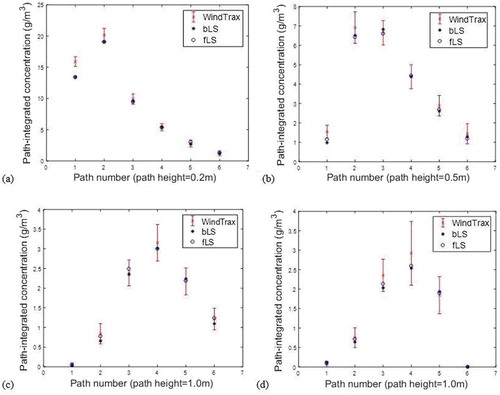
The concentrations calculated by the bLS and fLS models are inside the ranges of mean ± standard deviation (i.e., from mean – standard deviation to mean + standard deviation) calculated by WindTrax, except for the first path in the first setting (height of 0.2 m). This discrepancy was reported as a result of different initial particle velocities (Kljun, Rotach, and Schmid 2002). In our program, initial velocities follow a normal distribution. This treatment is simple because the correlation of the streamwise and vertical velocity components is neglected. As a result, unrealistic individual particle velocities may be produced. To solve this problem, a spin-up routine could be used (Kljun, Rotach, and Schmid 2002). The influence of initial velocities decreases with increasing dispersion distance. When that distance is larger than 0.5 m, all concentrations are inside the ranges of mean ± standard deviation calculated by WindTrax.

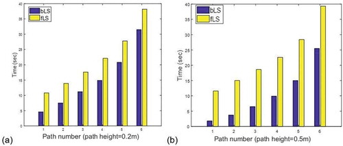
Figure 3 shows the computation time of the fLS and bLS models for different laser paths. The heights of laser path are 0.2 m in Figure 3a and 0.5 m in Figure 3b. For each path configuration, the fLS model is slower than the bLS model. Two factors affected the differences in the computation time. The first factor is the height difference between the source and the sensor. The source is located at ground level, which is a boundary where the wind speed is smaller than that at a higher level. Particles released from this ground-level surface spend longer time moving around the boundary area than released at a higher level. In contrast, particles released from sensor location at a higher level spend shorter time to move toward the source area. Another factor affecting the difference is the source-sensor distance. As the distance increases, the relative computation time difference caused by different releasing heights is reduced.

Figure 3. Computation time of bLS and fLS models for six laser paths with different heights: (a) Height = 0.2m. (b) Height = 0.5.

Problem of using “surface receptor”

Both bLS and fLS models can use a surface receptor, which is more accurate than using a box receptor due to the infinitely small height of the surface receptor (Flesch, Wilson, and Yee 1995). However, we found a constantly larger concentration calculated by bLS than that by fLS when running the simulation multiple times.

To get the average concentration and standard deviation, 8 simulations (each includes 500 repeated runs) were conducted using the bLS and fLS models, respectively. The source-receptor settings are the same as the configuration shown in Figure 1. Path 3 with a height of 0.5 m was used as the line sensor. In each run, 50,000 particles were released (a balance between the computation time and uncertainty). Figure 4a shows the average concentration and standard deviation for eight simulations. It shows that the standard deviation calculated by the bLS model is approximately two times larger than that by the fLS model.

Figure 4. (a) Average concentrations and standard derivations from 8 simulations for the bLS and fLS models (b) 500 concentration outputs (blue line) and the average concentration (red line) in one simulation.

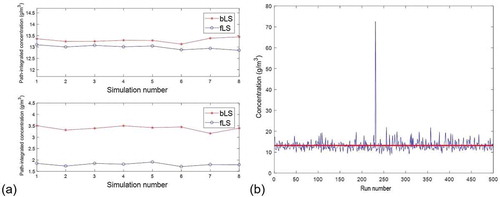
Figure 4b shows the concentrations calculated by the fLS model during 500 repeated runs with the same set of input parameters. It shows that there is an unusually large concentration value during the 225th run. To investigate this phenomenon, we checked the formulas for calculating the concentration, which is calculated as the ensemble-average particle “residence time”. Area sources can be represented using a volume with infinitely small height dh. The time duration that a particle passes through the source volume is $Min\left(\left|\frac{w}{u_j}\right|,\left|\frac{l}{v_j}\right|,\left|\frac{dh}{w_j}\right|,dt\right)=\frac{dh}{w_j}$. The concentration is (Flesch, Wilson, and Yee 1995)

(5) $C\left(\mathbf{x}\right)=\frac{1}{A_{src}dh}\frac{Q{A}_{src}}{N}\sum _{i=1}^N\sum _{j=0}^{M_i}\left|\frac{dh}{w_j}\right|=\frac{Q}{N}\sum _{i=1}^N\sum _{j=0}^{M_i}\left|\frac{1}{w_j}\right|.$(5)

where Q (g.m⁻².s⁻¹) is the mass flux of the area source, A_src is the area of the source, N is the total particle number, M_i is the times that the i^th particle appears inside the sensor volume. In this formula, dh is canceled and $\left|\frac{1}{w}\right|$ is used to calculate the concentration. In this case, an extremely low w generated from the random function may result in a large concentration value. In fact, a physical receptor must have a certain height dh. Particles will stay inside the receptor volume during one time step dt if they cannot pass through the receptor volume in dt. The chance that it will continue to keep this extremely small vertical velocity is very small, so we consider the constraint of $\left|\frac{dh}{w}\right|\le dt$ during one timestep. To decide a maximum value of $\left|\frac{1}{w}\right|$, a minimum value of dh has to be assigned. If a value of 10⁻⁶ m was used, this kind of outlier disappeared.

By assigning a certain height to a surface receptor, some unreasonable concentration values are removed. However, some values still tend to be larger than the normal values. We can see from Figure 4b that the variance above the line of mean concentration is larger than that below it. This is caused by using the source area as receptor in bLS model. When the particles touch the ground, they are bounced back into the air above the ground, in which case a particle passes the surface twice each time when it touches the ground. Therefore, the concentration is (Flesch, Wilson, and Yee 1995).

(6) $C\left(\mathbf{x}\right)=\frac{Q}{N}\sum _{i=1}^N\sum _{j=0}^{M_i}\left|\frac{2}{w_j}\right|.$(6)

Because $\left|\frac{2}{w}\right|$ is used in the backward model, the standard deviation is also approximately two times larger than that of the forward model.

Comparisons in non-steady-state atmosphere

Simulations with step-varying winds

In the simplest case, the simulated step-varying winds are used to drive the models. A point receptor is located at (5.0 m, 0 m, 0.5 m). The wind field is assumed to be horizontally homogeneous. 50,000 particles are released every 1.0 s during a period of 100 s. The concentration is calculated every second.

In Figure 5a, wind speed changes from high to low (2 m.s⁻¹ to 1 m.s⁻¹). The concentration generated by the fLS model decreases first then rises up to the level it should be in lower wind speed, while the concentration generated by the bLS model shows an opposite trend. In Figure 5b, wind speed changes from low to high (1 m.s⁻¹ to 2 m.s⁻¹). Opposite trends comparing to the high-to-low changing winds are shown.

Figure 5. Time-varying concentrations calculated using step-varying winds as model inputs: (a) Wind speed experiences a step change from 2.0 m/s to 1.0 m/s. (b) Wind speed experiences a step change from 1.0 m/s to 2.0 m/s.

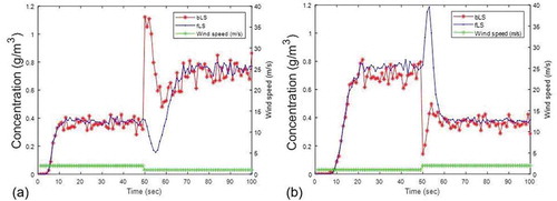
Because particles in the bLS model experience inverse time (from the future to the past), the common trend for both models is when the particles experience a low-to-high changing wind (Figure 5b for fLS and Figure 5a for bLS), the concentration increases first then decreases. This might be because more particles accumulated in the air between the source and receptor when at low wind speed than when at high wind speed. As soon as the wind speed rises, these particles reach the receptor quickly and cause an increase in the concentration. After they pass through, concentration drops back to normal value.

Simulations with sinusoidal-varying winds

Sinusoidal-varying winds are used to simulate a continuously varying wind. The wind speeds were generated using the following formula

(7) $U=Asin\left(2\pi ft\right)+B.$(7)

where U is the wind speed, A is the magnitude, f is the frequency, B is the offset.

When the magnitude, frequency and offset of the simulated winds are all fixed (1m/s, 0.05 Hz, 1.5 m/s). We found differences in the mean and the variation of the concentrations between the backward and forward models. Figure 6a shows an example of the calculated concentrations (source height is z₀, receptor height is 0.5 m). Figure 6b shows the 20 s moving window averaged concentration curves, in which the mean difference is exhibited. To investigate how each factor affects the differences, the height of the receptor, the magnitude and frequency of the winds are changed separately in the following simulations.

Figure 6. (a) Concentrations calculated by the bLS and fLS models with sinusoidal-varying winds as inputs. (b) 20 s moving window averaged concentrations in (a). (c) Normalized difference of mean concentrations between the bLS and fLS models (with fLS’ mean as reference) at different laser path heights. (d) Coefficients of variation of the concentrations of the bLS and fLS model at different laser path heights.

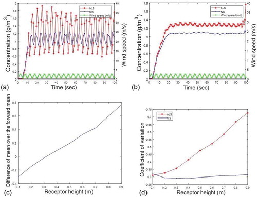
First, the height of the point receptor varied from 0.1 m to 0.9 m. In Figure 6c, the differences of mean concentrations (mean of backward concentrations minus mean of forward concentrations) relative to the mean of forward concentrations are plotted versus the receptor heights. When the height is below 0.3 m, the forward mean concentrations are larger than the backward concentrations. When the height is higher than 0.3 m, an opposite trend is shown. The relative difference of the means shows an increasing trend, which varies from −0.3 to 0.8, with increasing receptor height.

When the receptor height is increased, the variations of the concentrations show different trends. Figure 6d exhibits the coefficient of variation (CV, standard deviation over the mean) of the concentrations. The CV of forward concentrations shows a small variation, while that of backward concentrations shows a rapid increasing trend.

Second, the magnitude A changes from 0.0 to 1.4 m/s with other parameters fixed (f = 0.05 Hz, B = 1.5 m/s, receptor height = 0.5 m). In Figure 7a, the mean concentrations of the bLS model are larger than that of the fLS model. In Figure 7b, the relative difference of mean varies from 0.0 to 0.3, and a rising trend is shown. Figure 7b also shows the relative differences calculated with a receptor height of 0.9 m. In this case, the relative difference varies from 0.0 to 1.1.

Figure 7. (a) Mean concentrations calculated by the bLS and fLS models with different magnitudes of the sinusoidal varying winds. (b) Relative differences of mean concentrations between the fLS and bLS models with different magnitudes of the sinusoidal varying winds at heights of 0.5 m and 0.9 m. (c) Mean concentrations calculated by the bLS and fLS models with different frequencies of the sinusoidal varying winds. (d) Relative differences of mean concentrations between the fLS and bLS models with different magnitudes of the sinusoidal varying winds.

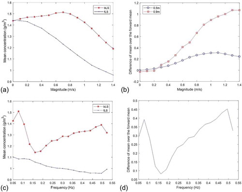
Third, the frequency of the winds changes from 0.05 to 0.5 Hz with other parameters fixed (A = 1.0 m/s, B = 1.5 m/s, receptor height = 0.5 m). In Figure 7c, the forward mean concentrations show a decreasing trend, while the backward mean concentrations does not have a monotonic trend. In Figure 7d, the relative difference of means shows a decreasing trend when the frequency is lower than 0.15 Hz. It increases from 0.05 to 0.45 when the frequency is larger than 0.15 Hz.

In these tests, the differences between the models are affected by the receptor height, magnitude, and frequency of the sinusoidal winds. The mean concentrations of the fLS model show decreasing trends with increasing receptor height, magnitude, and frequency of the sinusoidal winds. But the bLS model exhibits more complicated trends.The differences between the backward and forward mean concentrations generally show growing trends (when the frequency of the winds is larger than a critical value).

Methane release experiment

A methane release experiment was conducted in Okotoks, Canada to investigate the behaviors of the models driven by real wind fields, which is a part of the author’s project to quantify methane from fugitive area sources using optical remote sensing (ORS) and air dispersion modeling approach. The experiment is designed to simulate emissions from an area source under well-controlled conditions and uses open-path tunable diode laser (OP-TDL) as a line sensor which is deployed very close to the source (2–50 m). The path-integrated concentration (PIC) and the wind data with a high frequency were recorded.

The ORS system consists of an OP-TDL methane analyzer (Boreal Gas Finder 3), a pan-tilt positioner, and a retroreflector array. The simulated area source (4.0 m × 4.0 m) was constructed by polyvinyl chloride (PVC) pipes with a diameter of 18 mm. Small holes were drilled along the pipe with a diameter of 1 mm and 0.3 m spacing between the holes. A methane cylinder with a 99.9% purity was connected to the manifold through a regulator and flowmeter. The flow rate was controlled at 2 L/min. The cylinder valve was manually adjusted every 1–2 min to maintain a constant flow rate.

Wind speeds were recorded with a three-dimension sonic anemometer (Campbell Scientific CSAT3B) located at the height of 1.35 m with a sampling frequency of 20 Hz. Path-integrated concentrations (PICs) of methane were measured by the OP-TDL methane analyzer with a sampling frequency of 1 sample per 4 s. The releasing process lasted for 30 min. The weight of the cylinder was measured before and after the release to calculate an averaged emission rate Q_m. Background methane concentration (C_b) was also measured before and after the release.

First, the emission rates were calculated with one 15-min averaged wind. Parameters are summarized in Table 1, which are calculated following the formulas in Flesch et al. (2004). The emission rates calculated by the fLS and bLS models are the same: Q_model = 0.0244 g/m².s. The recovery ratio Q_model/Q_m is 0.7922. This means the model overestimates the emission rate about by 20%. This trend is in agreement with the tests reported by Gao, Desjardins, and Flesch (2009), under the condition that the source-receptor distance is short.

Table 1. Parameters of the controlled-release experiment. ${\sigma }_{u,v,w}/u^{\ast }$ are turbulent fluctuations.

Parameter	value	Parameter	value
Along-wind velocity (U)	1.6334 m.s^−1	Friction velocity (u*)	0.4014 m.s^−1
Wind direction	108.3867°	σu/u*	2.0848
Temperature (T)	26.0917°	σv/u*	1.5664
Obukhov length (L)	55.4 m	σw/u*	1.2827
Roughness length (z0)	0.1195 m	Measured emission rate (Qm)	0.0308 g.m^−2.s^−1
Measured concentration (Cm)	3.58 ppm	Background concentration (Cb)	1.8 ppm
Path length	57 × 2 m	TDL & mirror location	(0 m, -49 m, 2.0 m), (0 m, 8 m, 2.0 m)
Source area	4 × 4 m^2	Source location (Left-bottom corner)	(3.0 m, -0.8 m, z0)

Next, time-varying winds were used to drive the bLS and fLS models. The average interval of wind is set to 30 s, as the source-receptor distance is very short (2 m to 50 m). The averaged winds change every 4 s according to TDL’s sampling interval. The calculated and measured time-varying concentrations are shown in Figure 8. The outputs from the fLS and bLS model have correlation coefficient of 0.95. The correlation coefficient between the model calculated and measured values is 0.70.

Figure 8. Measured and model-predicted concentrations.

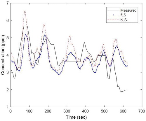
The emission rates are determined through a least square fit between the measured curve and model-predicted curve. The bLS model estimates 10–35% larger peak concentrations than that by the fLS model under the same emission rate. The differences between the two predicted concentrations relative to the concentrations predicted by the fLS model vary from −0.1 to 0.3. This means the relative differences are within ±30% of the fLS predicted values. For the fLS model, the best-fitted Q_f is 0.0356, and the recovery ratio is 1.1558. For the bLS model, the best-fitted Q_b is 0.0298, and the recovery ratio is. 0.9675. (Q_b -Q_f)/Q_f ×100% is −4%. These results are better than when using a constant 15-min averaged wind as input (recovery rate is 0.7922).

Conclusion

We compared the fLS and bLS models in micro-scale dispersion processes under different atmosphere conditions. In a steady-state wind flow, with the assumption of uniform source and horizontally homogeneous atmosphere, the two models are equivalent with each other in many features, including estimating the concentration at a point, using surface receptor, and calculating concentration footprints before knowing the source and receptor geometry. The bLS model has better computational efficiency by releasing particles from a higher level above the ground. However, the standard deviation of the concentration calculated by the bLS model is approximately two times larger than that of the fLS model, which is caused by using a “surface” receptor with zero thickness.

In non-steady-state conditions, the differences between these two models are affected by many factors (receptor height, fetch, wind speed, wind direction, wind patterns, etc.). It is difficult to evaluate the differences caused by all these factors at the same time, and the comparisons are usually case-specific. Instead, we investigate the influences of each individual factor. In the simplest case, step-varying winds are simulated to drive the models. Concentrations calculated by the two models show opposite trends during the step-change process. Then, sinusoidal-varying winds are simulated to investigate the influences of the receptor height, magnitude, and frequency of the wind. The normalized differences of the means concentration mainly increase with the receptor height.

In applications, the differences between these two models are caused by the superposition effects due to all the factors. Model behaviors driven by a real wind field were studied through a controlled methane release experiment. Time-varying winds were recorded and used to drive the models. Predicted concentrations from both models show similar trends with the correlation coefficient of 0.70 between the measured concentrations by the two models. The emission rates are determined through a least square fit between the measured curve and model-predicted curve. The bLS model estimates larger peak concentrations than that by the fLS model under the same emission rate. The differences of the concentrations are within 30% of the fLS predicted values under the experiment setting. The best-fitted results of the fLS and bLS models have recovery ratios of 1.1558 and 0.9675, respectively, which are better than that using a constant 15-min averaged wind (0.7922). The relative difference between the recovery ratios is only 4%. Based on these results, we conclude that the bLS model generally agrees with the fLS model driven by real wind fields in the micro-scale dispersion.

Acknowledgment

The work was supported by the following grants: John R. Evans Leaders Fund (JELF) and Infrastructure Operating Fund (IOF) from Canada Foundation for Innovation (CFI), University Research Grant Committee (URGC) seed grant, and the New Faculty Start-up grant from University of Calgary.

Disclosure statement

No potential conflict of interest was reported by the authors.

Additional information

Funding

This work was supported by the Canada Foundation for Innovation [35468]; University of Calgary [1050666].

Notes on contributors

Sheng Li

Sheng Li ([email protected]) is a Ph.D. candidate in Environmental Engineering at the University of Calgary, Calgary, Canada.

Ke Du

Ke Du ([email protected]) is an associate professor at the Department of Mechanical and Manufacturing Engineering, University of Calgary, Calgary, Canada.

References

- Batchelder, H. 2006. Forward-in-time-/backward-in-time-trajectory (fitt/bitt) modeling of particles and organisms in the coastal ocean. J. Atmos. Oceanic Technol. 23 (5):727–41. doi:10.1175/JTECH1874.1.
- Bieringer, P. E., G. S. Young, L. M. Rodriguez, A. J. Annunzio, F. Vandenberghe, and S. E. Haupt. 2017. Paradigms and commonalities in atmospheric source term estimation methods. Atmos. Environ. 156:102–12. doi:10.1016/j.atmosenv.2017.02.011.
- Cai, X., G. Peng, X. Guo, and M. Y. Leclerc. 2008. Evaluation of backward and forward Lagrangian footprint models in the surface layer. Theor. Appl. Climatol. 93:207–23. doi:10.1007/s00704-007-0334-0.
- Draxler, R. R. 2006. The use of global and mesoscale meteorological model data to predict the transport and dispersion of tracer plumes over Washington, DC. Weather Forecast 21 (3):383–94. doi:10.1175/WAF926.1.
- Eckhardt, S., M. Cassiani, N. Evangeliou, E. Sollum, I. Pisso, and A. Stohl. 2017. Source–receptor matrix calculation for deposited mass with the Lagrangian particle dispersion model FLEXPART v10.2 in backward mode. Geosci. Model Dev. 10:4605–18. doi:10.5194/gmd-10-4605-2017.
- Flesch, T. K., J. D. Wilson, and E. Yee. 1995. Backward-time lagrangian stochastic dispersion models and their application to estimate gaseous emissions. J. Appl. Meteorol. 34:1320–32. doi:10.1175/1520-0450(1995)034<1320:BTLSDM>2.0.CO;2.
- Flesch, T. K., J. D. Wilson, L. A. Harper, B. P. Crenna, and R. R. Sharpe. 2004. Deducing ground-to-air emissions from bbserved trace gas concentrations: A field trial. J. Appl.Meteorol. 43:487–502. doi:10.1175/1520-0450(2004)043<0487:DGEFOT>2.0.CO;2.
- Flesch, T. K., V. S. Baron, J. D. Wilson, D. W. T. Griffith, J. A. Basarab, and P. J. Carlson. 2016. Agricultural gas emissions during the spring thaw: Applying a new measurement technique. Agric. Forest Meteorol. 221:111–21. doi:10.1016/j.agrformet.2016.02.010.
- Gao, Z., R. L. Desjardins, and T. L. Flesch. 2009. Comparison of a simplified micrometeorological mass difference technique and an inverse dispersion technique for estimating methane emissions from small area sources. Agric. For. Meteorol. 149:891–98. doi:10.1016/j.agrformet.2008.11.005.
- Gifford, F. A. 1959. Computation of pollution from several sources. Int. J. Air Poll. 2:109–10.
- Goodrick, S. L., G. L. Achtemeier, N. K. Larkin, Y. Liu, and T. M. Strand. 2013. Modelling smoke transport from wildland fires: A review. Int. J. Wildland Fire 22:83–94. doi:10.1071/WF11116.
- Harper, L. A., T. K. Flesch, J. M. Powell, W. K. Coblentz, W. E. Jokela, and N. P. Martin. 2009. Ammonia emissions from dairy production in Wisconsin. J. Dairy Sci. 92:2326–37. doi:10.3168/jds.2008-1753.
- Hegarty, J., R. R. Draxler, A. F. Stein, J. Brioude, M. Mountain, J. Eluszkiewicz, T. Nehrkorn, F. Ngan, and A. Andrews. 2013. Evaluation of Lagrangian particle dispersion models with measurements from controlled tracer releases. J. Appl. Meteorol. Climatol. 52 (12):2623–37. doi:10.1175/JAMC-D-13-0125.1.
- Kljn, N., P. Kastner-Klein, E. Fedorovich, and N. W. Rotach. 2004. Evaluation of Lagrangian footprint model using data from wind tunnel convective boundary layer. Agric. Forest Meteorol. 127:189–201. doi:10.1016/j.agrformet.2004.07.013.
- Kljun, N., N. W. Rotach, and H. P. Schmid. 2002. A three-dimensional backward Lagrangian footprint model for a wide range of boundary-layer stratifications. Boundary-Layer Meteorol. 103:205–26. doi:10.1023/A:1014556300021.
- Lin, J. C., C. Gerbig, S. C. Wofsy, A. E. Andrews, B. C. Daube, K. J. Davis, and C. A. Grainger. 2003. A A near‐field tool for simulating the upstream influence of atmospheric observations: The Stochastic Time‐Inverted Lagrangian Transport (STILT) model.J. Geophys. Res. 108 (D16):4493. doi:10.1029/2002JD003161.
- Lin, J. C., D. Brunner, and C. Gerbig. 2011. Studying atmospheric transport through Lagrangian models. Eos Trans. AGU. 92 (21):177. doi:10.1029/2011EO210001.
- McGinn, S. M., T. K. Flesch, B. P. Crenna, K. A. Beauchemin, and T. Coates. 2007. Quantifying ammonia emissions from a cattle feedlot using a dispersion model. J. Environ. Qual. 36:1585–90. doi:10.2134/jeq2007.0167.
- Riddick, S. N., S. Connors, A. D. Robinson, A. J. Manning, P. S. D. Jones, D. Lowry, E. Nisbet, R. L. Skelton, G. Allen, J. Pitt, et al. 2016. Estimating the size of a methane emission point-source at different scales: From local to landscape. Atmos. Chem. Phys. 17:7839–51. doi:10.5194/acp-17-7839-2017.
- Rodean, H. 1996. Stochastic Lagrangian models of turbulent diffusion. Meteor. Mon. 48:1–84. doi:10.1175/0065-9401-26.48.1.
- Schmid, H. P. 2002. Footprint modeling for vegetation atmosphere exchange studies: A review and perspective. Agric. Forest Meteorol. 113:159–83. doi:10.1016/S0168-1923(02)00107-7.
- Seibert, P., and A. Frank. 2004. Source-receptor matrix calculation with a Lagrangian particle dispersion model in backward mode. Atmos. Chem. Phys. 4:51–63. doi:10.5194/acp-4-51-2004.
- Stohl, A., C. Forster, A. Frank, P. Seibert, and G. Wotawa. 2005. Technical note: The Lagrangian particle dispersion model FLEXPART version 6.2. Atmos. Chem. Phys. 5:2461–74. doi:10.5194/acp-5-2461-2005.
- Thomson, D. J. 1987. Criteria for the selection of stochastic models of particle trajectories in turbulent flows. J. Fluid Mech. 180:529–56. doi:10.1017/S0022112087001940.
- Thomson, D. J., and J. D. Wilson. 2012. History of the Lagrangian stochastic model for turbulent dispersion. Lagrangian Model. Atmos. American Geophys. Union 200:19–36.
- Wilson, J. D., and T. K. Flesch. 1993. Flow boundaries in random flight dispersion models: Enforcing the well-mixed condition. J. Appl. Meteor. 32:1695–707. doi:10.1175/1520-0450(1993)032<1695:FBIRFD>2.0.CO;2.
- Wilson, J. D., T. K. Flesch, and L. A. Harper. 2001. Micro-meteorological methods for estimating surface exchange with a disturbed windflow. Agric. Forest Meteorol. 107:207–25. doi:10.1016/S0168-1923(00)00238-0.