Assessment of mobile source air toxics in an Environmental Justice Denver community adjacent to a freeway

ABSTRACT

Air pollutant concentrations are often higher near major roadways than in the surrounding environments owing to emissions from on-road mobile sources. In this study, we quantified the gradient in black carbon (BC) and air toxics concentrations from the I-70 freeway in the Elyria-Swansea environmental justice neighborhood in Denver, Colorado, during three measurement campaigns in 2017–2018. The average hourly upwind-downwind gradient of BC concentrations from the roadway was 500–800 ng/m³, equal to an increment of approximately 30-80% above local background levels within 180 m of the freeway. When integrated over all wind directions, the gradients were smaller, approximately 150–300 ng/m³ (~11-18%) over the course of nearly four months of measurements. No statistically significant gradient in air toxics (e.g., benzene, formaldehyde, etc.) was found, likely because the uncertainties in the mean concentrations were larger than the magnitude of the gradient (<25%). This finding is in contrast to some earlier studies in which small gradients of benzene and other VOCs were found. We estimate that sample sizes of at least 100 individual measurements would have been required to estimate mean concentrations with sufficient certainty to quantify gradients on the order of ±10% uncertainty. These gradient estimates are smaller than those found in previous studies over the past two decades; more stringent emissions standards, the local fleet age distribution, and/or the steady turnover of the vehicle fleet may be reducing the overall impact of roadway emissions on near-road communities.

Implications: Gradients of near-road pollution may be declining in the near-road environment as tailpipe emissions from the vehicle fleet continue to decrease. Near-road concentration gradients of mobile source air toxics, including benzene, 1,3-butadiene, and ethylbenzene, will require higher sample sizes to quantify as emissions continue to decline.

Introduction

In recent years, near-road air quality has been the focus of many monitoring and modeling studies (Barzyk et al. 2015; Bates et al. 2018; Ginzburg et al. 2015; Parvez and Wagstrom 2019; Saha, Khlystov, and Grieshop 2018a) due to the potential negative health impacts of air pollution from major roadways and the large portion of the population residing close to major roadways (Brugge, Durant, and Rioux 2007; Ghosh et al. 2017, 2016; Health Effects Institute 2010; Health Effects Institute Air Toxics Review Panel 2007; Wilhelm et al. 2011). Several studies have shown that daytime pollutant concentrations can be many times greater than background concentrations within 150 m of a major roadway, while decreasing rapidly with increasing distance from the roadway. (Baldauf et al. 2008; Hagler et al. 2009; Jeong et al. 2019; Oakes et al. 2016; Parvez and Wagstrom 2019; Riley et al. 2014; Saha et al. 2018b; Zhu et al. 2002b, 2004). Observational studies have shown that there is a significant gradient of black carbon (BC), ultrafine particles, and nitrogen dioxide (NO₂) concentrations next to roadways, and a smaller gradient of fine particulate matter (PM_2.5) (Karner, Eisinger, and Niemeier 2010; Saha et al. 2018b). Furthermore, concentrations of certain pollutants measured in the near-road environment are heavily influenced by the fleet mix of vehicles traveling on the adjacent roadway; for example, ultrafine particles and BC concentrations are positively correlated to diesel-fueled vehicles (Brown et al. 2014; Dallmann et al. 2012; Dallmann and Harley 2010; Kleeman et al. 2009; Patterson and Harley 2019; Riddle et al. 2008). Several studies have also found significant negative health impacts, such as reduced lung function, low birth weights, and increased asthma and risk of heart failure, for individuals living within 300 m of major roadways (Brandt et al. 2014; Ghosh et al. 2016; Health Effects Institute 2010; Urman et al. 2014).

Hazardous air pollutants (HAPs), also called air toxics, are ambient air pollutants that pose a wide range of threats to human health. Section 112 of the Clean Air Act (CAA), as amended in 1990, lists 189 HAPs and mandates regulations to control their emissions. Scientific studies have shown that a number of these air toxics are carcinogenic, and many are associated with a wide variety of negative health impacts, including adverse effects on reproductive, developmental, and neurological health (Clark-Reyna, Grineski, and Collins 2016; Loh et al. 2007; Rosenbaum et al. 1999; Wilhelm et al. 2011; Woodruff et al. 1998, 2000). Mobile source air toxics are air toxics that are emitted through the combustion cycle of motor vehicles. The 2014 National Air Toxics Assessment provides an overview of which HAPs provide the greatest carcinogenic exposure risk, and which emissions sources contribute to that risk – showing that mobile source emissions from light duty vehicles, heavy duty vehicles, and diesel vehicles remain a significant contributor to cancer risk (U.S. Environmental Protection Agency 2014b, 2015a). Benzene is a key hazardous air pollutant and mobile source air toxic (MSAT) that is the focus of the measurements and modeling here, as it classified as a known human carcinogen for all routes of exposure under the proposed revised Carcinogen Risk Assessment Guidelines (Fruin et al. 2001; Health Effects Institute Air Toxics Review Panel 2007; Skov et al. 2001; Smith 2010; U.S. Environmental Protection Agency 1996, 2018; Woodruff et al. 1998). Other potentially important sources of benzene and other HAPs in the area include emissions from manufacturing, petrochemical and chemical facilities, waste incinerators, non-road mobile sources, and stationary engines.

Mobile source emissions have been a regulatory target of successive rulemaking procedures following the statutory mandate of the 1990 amendments to the CAA (https://www.epa.gov/mobile-source-pollution/regulations-reduce-mobile-source-pollution). Between 2000 and 2014, the U.S. Environmental Protection Agency (EPA) promulgated three major regulations: Tier 2 Motor Vehicle Emissions Standards and Gasoline Sulfur Control Requirements; Control of Hazardous Air Pollution from Mobile Sources; and Tier 3 Motor Vehicle Emission and Fuel standards (U.S. Environmental Protection Agency 2000, 2014a, 2007). Implementation of Tier 3 standards for motor vehicle emissions and fuel composition are ongoing, and tailpipe emissions standards “generally phase in between model years 2017 and 2025.” This regulatory framework has led to significantly lower emissions from the traffic sector overall (McDonald et al. 2013; Reid et al. 2016).

A review study by Karner et al. examined the spatial gradient of pollutant concentrations over a 500-meter distance from the edge of the roadway, relative to the background and relative to the edge of the roadway, synthesizing results from numerous studies prior to 2010 (Karner, Eisinger, and Niemeier 2010). They found that some volatile organic compounds (VOCs), including ethane, propane, n-butane and n-hexane, showed a rapid decline in concentration (>50%) starting 150 meters from the roadway. They also present a black carbon gradient of ~50%, 150 meters from the roadway, and show that total PM_2.5 has a much weaker gradient, 15% over 150 meters. Other studies have focused on the modeled and measured gradient of vehicle emissions versus distance to road, showing gradients of benzene, BC, and ultrafine particles, generally focused on downwind conditions only (Baldauf et al. 2008; Chang et al. 2015; Parvez and Wagstrom 2019; Riley et al. 2014; Saha et al. 2018b; Zhu et al. 2002b, 2004).

As the health effects from environmental exposure to criteria pollutants in the United States have been substantially reduced over the past four decades (U.S. Environmental Protection Agency 2019), an increased focus has been placed on the equity of exposure and to the environmental and health-related outcomes related to the location of emissions sources as reflected in environmental justice concerns. Nationally, 19% of the population lives within 500 meters of high traffic volume roads, which are defined as having greater than 25,000 annual average daily traffic (AADT) based on 2010 census data (Rowangould 2013). Studies have found inequities of exposure to air toxics in the near-road population with respect to race, community segregation, and socioeconomic status (Houston, Krudysz, and Winer 2008; Morello-Frosch and Shenassa 2006) as well as race and income (Apelberg, Buckley, and White 2005; Miranda et al. 2011; Pope and Dockery 2006; Rowangould 2013).

The Elyria-Swansea neighborhood is an environmental justice community located in central Denver near the convergence of Interstate Highways 70 and 25. I-70 runs east-west through the neighborhood, and a major rail line runs southwest-northeast through the neighborhood. The community in the vicinity of Swansea Elementary school is the domain of this study and ranks in the 86th percentile for PM_2.5 exposure, 96th percentile for diesel PM exposure, and in the 97th percentile for traffic proximity and volume, according to EPA’s EJScreen EJ Index data (available interactively through https://ejscreen.epa.gov/mapper/). Higher percentiles mean that the census blocks of the Elyria-Swansea neighborhood are among the worst in the U.S. for these pollution categories (U.S. Environmental Protection Agency 2017). Total AADT on I-70 is 153,000. A major redevelopment project was proposed to change the roadway configuration of I-70 as it transits this neighborhood (see https://www.codot.gov/projects/i70east). Currently, I-70 is an elevated viaduct approximately 30 feet higher than the surrounding communities. As part of the I-70 redevelopment project beginning in 2019, the I-70 viaduct will be replaced with a 30 foot below-grade highway. A 990 foot long stretch adjacent to Swansea Elementary School will be covered by a 4-acre cap and ground-level parkland. One of the major goals of this study is to provide baseline concentration measurements of pollution gradients around the elevated roadway configuration prior to redevelopment. It is anticipated that a second monitoring study will be performed after completion of the I-70 redevelopment project to attempt to quantify the changes in pollution concentrations.

In this work, we present results from measurements of black carbon and air toxics at multiple temporary community sites perpendicular to I-70 in the Elyria-Swansea neighborhood, focused on the area at and around Swansea Elementary School. We use these measurements to determine concentrations of BC and air toxics, and the extent to which concentrations are higher with increasing proximity to the freeway. Measured results are compared to modeling of benzene with AERMOD. As part of work to understand the impact of a future expansion of I-70, the Denver Department of Public Health and Environment (DDPHE) conducted modeling of PM_2.5, NO₂, and benzene for the Elyria-Swansea neighborhood. This was presented in The Going One Step Beyond in North Denver study (Thomas, Williams, and Bain 2007), which is a combined neighborhood and project scale modeling assessment, to compare a 2011 baseline year with 2035 predicted conditions for the expanded and fully built out I-70 (Central 70) project. Benzene in Denver is mostly emitted from motor vehicle exhaust in addition to other sources such as gasoline service stations, oil and gas activities and refining, and wood burning.

Experiments

Spatial domain

Air pollution monitoring of air toxics (carbonyls, VOCs, and BC) was conducted over three campaigns on a north-south axis along Elizabeth Street and Thompson Court perpendicular to I-70, focused on the area at and around Swansea Elementary School, which employed a playground adjacent to I-70. Monitoring stations were sited on or near the Swansea Elementary School campus north of the highway and at sites on rooftops and in parks south of the highway. Figure 1 shows the study domain along with monitoring site locations for Campaigns I, II, and III. Monitoring site locations for Campaigns I and II are shown in blue, and those for Campaign III are shown in red.

Figure 1. Monitoring site locations for Campaigns I and II (left) and Campaign III (right)

Monitoring campaigns

The study involved three monitoring periods. Campaigns I and II had identical monitoring methods and site locations. Campaign III deployed measurements at different site locations as a result of logistical constraints. In all cases, the goal was to identify concentrations in the near-road environment that were representative of concentration exposures experienced in the community and elementary school during school periods.

• Campaign I was run from October 25, 2017, through November 25, 2017.

• Campaign II was run from February 2, 2018, through March 2, 2018.

• Campaign III was run from September 14, 2018, through October 29, 2018.

Table 1 lists the site locations, elevations, names, and measurement methods deployed in Campaigns I and II. Table 2 lists the site locations, elevations, names, and measurement methods deployed in Campaign III. Note that in Campaign III, site 2N_a only operated from September 14 through 25, 2018. That site was then relocated to the site labeled 2N_b, which operated from September 26 through October 29, 2018. BC was measured by microAeths at five near-roadway sites in Campaigns I and II. Sites 1S and 1N were closest to the roadway (within 20 meters of the nearest lane of traffic on I-70). Sites 2S, 3N, and 5N were all more than 100 meters from the nearest lane on I-70. Site 2S was located on top of a building and is elevated relative to other sites in the measurement study.

Table 1. Site locations and measurements deployed in Campaigns I and II

Site Name	Distance from I-70 (m)	Latitude	Longitude	Elevation (m)	MicroAeth	Carbonyls	Met
1N	17	39.78034	104.9564	1582	x	x
1S	16	39.77983	104.95488	1583	x	x
2N	146	39.78066	104.9561	1582	x	x
2S	127	39.77877	104.9547	1586	x	x
3N	102	39.78111	104.95611	1582	x	x
4N	177	39.78137	104.9554	1582		x	x
5N	177	39.78178	104.9561	1581	x	x

Table 2. Site locations and measurements deployed in Campaign III

Site Name	Distance from I-70 (m)	Latitude	Longitude	Elevation (m)	MicroAeth	VOCs	Met
1S	16	39.779834	104.95488	1583	x	x
1N*	91	39.781	104.9554	1582	x	x	x
2N_a	146	39.781	104.9559	1582	x	x
3N	102	39.7811	104.9561	1582	x	x
2N_b	148	39.7815	104.956	1582	x	x
4N	177	39.7818	104.9561	1582	x	x

Notes. *Site 1N was not at the same location as in Campaigns I and II due to inaccessibility of the location on the school playground during Campaign III.

Monitoring methodology

Four unique measurement methods were employed during the campaigns.

1. BC measurements were made in all three campaigns using microAethalometers. BC concentrations are corrected for optical attenuation using the approach documented in Kirchstetter and Novakov (2007).

2. Meteorological measurements were made in all three campaigns, most importantly including wind speed and wind direction.

3. Carbonyl cartridge samples were collected in Campaigns I and II using EPA method TO-11.

4. Summa canisters were used to collect VOCs in Campaigns I–III and analyzed using GC-MS EPA method TO-15 (U.S. Environmental Protection Agency 1999b).

VOC results from Campaign I, identified midway through campaign II (Feb 2018), were suspected to be of questionable accuracy due to a laboratory issue. Three split samples to different laboratories late in campaign II confirmed this. This was a primary driver for conducting Campaign III, since VOC concentrations are important to the surrounding communities.

Black carbon – BC concentrations were determined using the Aethlabs AE51 personal microAeth Aethalometers. The microAeth samplers are fully self-contained instruments with a built-in pump, flow control, and data-storage; see https://aethlabs.com/microaeth/ae51/overview. Data were collected at five-minute intervals in all campaigns but have been aggregated up to hourly means for hours with at least 75% completeness of valid measurements (status indicator = 0, concentration ≥ 0 ng/m³). Cai et al. found high reproducibility among six microAeth units (relative standard deviation of 8%) and good agreement with the rack-mounted Aethalometer AE33 unit (R = 0.92, slope = 1.01) (Cai et al. 2014) Cheng and Lin found differences between the AE51 and an AE31 model Aethalometer of up to 14% but overall good agreement (R² = 0.97 without AE31 data treatment) (Cheng and Lin 2013). Viana et al. found similar results comparing the AE51 to elemental carbon measurements from a Thermo Multi-Angle Absorption Photometer (MAAP), with R² values between five AE51s and the MAAP ranging between 0.75 and 0.85 with slopes between 0.75 and 1.15 (Viana et al. 2015). The AE51 has been used in multiple studies for determining personal exposure as well as BC concentrations inside residences and in ambient environments (Lovinsky-Desir et al. 2018; Rivas et al. 2016).

Meteorology – A standard suite of meteorological measurements were collected at one monitoring site during each campaign. Meteorological data collected included resultant wind speed, resultant wind direction, relative humidity, barometric pressure, and temperature. We note that the siting for the meteorological station did not necessarily meet EPA requirements for siting due to a limited fetch and obstructions from nearby trees and buildings.

Carbonyls – Carbonyl compounds were analyzed from samples collected on an every-other-day and weekly schedule using dinitrophenylhydrazine (DNPH)-coated sorbent cartridges following EPA’s Method TO-11a (U.S. Environmental Protection Agency 1999a). These samples were sent to an analytical laboratory for analysis using high-performance liquid chromatography (HPLC).

VOCs – VOCs were collected for 24 hours on an every-other-day schedule using SUMMA stainless steel canisters following EPA method TO-15 (U.S. Environmental Protection Agency 1999b). Collected samples were sent to a local university laboratory for analysis using gas chromatograph mass spectrometry (GC-MS).

Modeling methodology

The AERMOD dispersion model was used to estimate benzene concentrations from both polygon (area and nonroad) and link-based (highway) sources. Most assumptions and model settings were kept the same as in the 2016 North Denver study (Thomas, Ogletree, and Clay 2016). Polygon emissions were calculated by allocating the 2011 NEI county benzene emissions to the polygon transportation analysis zones (TAZs). The allocation surrogates, obtained from the Denver Regional Council of Governments (DRCOG) data, included vehicle miles traveled (VMT), population and/or population density, number of oil and gas wells, and miles of railroad tracks. Area sources were assumed not to change between 2011 and 2018 in the model; this assumption is likely to result in a negligible impact on total emissions in each polygon (~1–2% difference in total emissions if NEI 2014 rates were used). The 2004 meteorological data used in this study were collected at the nearby Rocky Mountain Arsenal (surface) and the former Denver Stapleton Airport (upper air) and were again used in this model.

In the 2016 North Denver study, the Motor Vehicle Emission Simulator (MOVES2014) model was used to estimate county level annual emissions of benzene (as well as PM_2.5 and NO_x) for 2011, 2015, 2020, 2025, 2030, and 2035 (U.S. Environmental Protection Agency 2015b, 2016). Since the year 2018 was not explicitly modeled, the 2018 county annual emissions of benzene were calculated by interpolation between 2015 and 2020. The MOVES results showed that the 2011 on-road emissions of benzene were reduced by 57% in 2018. This reduction factor was used to estimate the polygon 2018 benzene emissions. Benzene emissions from non-road, railroad and upstream oil and gas sources were assumed to be reduced from 2011 to 2018. Reduction factors based on professional judgment were used: 10% reduction in non-road, 10% reduction in railroad emissions, and 25% reduction in upstream oil and gas emissions. There are relatively few emissions from upstream oil and gas in Denver County as compared to counties to the north (20–90 miles away). The AERMOD-modeled impacts in Denver from upstream oil and gas are negligible. There is an oil refinery approximately 1.5 miles to the north of the monitoring study area. Given that prevailing winds are more frequently from the south, the influence of the oil refinery is expected to be intermittent; chemical fingerprint analysis is used to attempt to identify possible source impacts from this the refinery. Given both 2035 and 2018 (interpolated) annual benzene emissions from MOVES, as well as link emissions for 2035, the link emissions for 2018 were estimated using a linear relationship. For onroad emissions, the project links were modeled explicitly based on forecast VMT. However, there are also emissions from local roads and other sectors in the city not captured in forecasts. For transportation analysis zones (TAZs) bordering the area around Swansea Elementary school, all emissions were included (onroad, nonroad, area, and point). For TAZs where the I-70 on-network highway links fell within that TAZ, 10% of previously processed onroad emissions were retained to account for estimated contributions from traffic on local roads and connectors, mainly in the surrounding neighborhood. The link-based on-road emissions were then modeled on top of the remaining emissions.

The study estimated emissions and concentrations of PM_2.5, NO₂, and benzene for two scenarios: winter (January) and summer (July) concentrations. Benzene results are presented here.

It is important when interpreting the results from this project to understand the local meteorology. The South Platte River is about one mile west of the project boundary shown in Figure 1. Typically, winds are from the south during the overnight and early morning hours, following the river drainage. Therefore, locations north of the highway are expected to see higher impacts during those times. As the mountains to the west of Denver absorb sunlight and the temperature rises, a low pressure zone is created (i.e., the Denver Cyclone) and winds start originating from the northeast by early afternoon, especially during the warmer months. On average, it is more likely that a site north is downwind of the highway in the early morning hours and then upwind of the highway in the afternoon and early evening hours. This will mask concentration gradients from the highway unless concentrations are binned by wind direction.

Results

Black carbon in Campaigns I, II, and III

Near-road gradients can be examined as either acute phenomena that occur within the context of a local wind field, or as a cumulative chronic gradient that integrates over all possible wind directions. Both types of exposures can be important, as people living, working, and going to school next to roadways have different activity patterns that may be affected as a result of their movements. We examined both the chronic integrated exposures and the acute maximum gradients when winds are from the roadway.

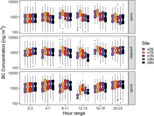
Diurnal patterns of BC concentrations segregated into three wind bins are shown in Figures 2 and 3. Wind bins are 120 degree arcs―winds from the north, winds in two 60-degree arcs from the east or west parallel to the freeway, and winds from the south. Hours are binned in 4 hour aggregates to increase the sample size, reduce notch sizes, and better illustrate central tendencies in patterns. The concentration gradients were characterized across all hours when segregated by wind direction and are shown in Tables 3 and 4 for Campaigns I and II, and Campaign III, respectively. Boxplots were generated using the R tidyverse ggplot2 library (https://ggplot2.tidyverse.org/reference/geom_boxplot.html); boxes correspond to the interquartile range (IQR), whiskers extend to 1.5*IQR, and individual outliers are outside the 1.5*IQR. Notches are 1.58*IQR/sqrt(n), which gives a roughly 95% confidence interval for comparing medians.

Table 3. Summary average BC concentrations for Campaigns I and II, segregated by wind direction

		Average BC Concentration (ng/m^3)
Site	Distance (m) from I-70	Winds from the South	Parallel Winds	Winds from the North	All Wind Directions
1S	16	1946	1842^a	1944	1916^a
2S	127	1646	1271	1496	1490
1N*	17	2133^c	1581	1340	1694^b
3N	102	2191^c	1481	1229	1644
5N	177	2031^c	1292	1190	1519

Notes. ^aThe distribution of concentrations for Site 1 S was significantly higher at the 95% confidence level than for all other sites.

^bThe distribution of concentrations for Site 1N was significantly higher at the 95% confidence level than for Site 2S and Site 5N.

^cThe distribution of concentrations for Sites 1N, 3N, and 5N were all higher than for Sites 1S and 2S at the 95% confidence level.

Table 4. Summary average BC concentrations for Campaign III, segregated by wind direction

		Average BC Concentration (ng/m^3)
Site	Distance (m) from I-70	Winds from the South	Parallel Winds	Winds from the North	All Wind Directions
1S	16	1390^a	1586^a	1798^a	1578^a
1N	91	1970	1197	1006	1483
2N	146	2065	1216	1004	1436
3N	102	1610	1051	903	1254^b
4N	177	1727	1072	949	1334

Notes. ^aThe distribution of concentrations for Site 1S was significantly higher at the 95% confidence level than for all other sites when winds blew from the north, were parallel, and under All Wind Directions. It was statistically significantly lower when winds blew from the south.

^bThe distribution of concentrations for Site 3N was significantly lower at the 95% confidence level than for Site 1S and 1N.

Figure 2. Campaign I and II gradients in hourly average binned BC concentrations (ng/m³) measured by microAeths when winds are from the north (top), parallel (middle), and south (bottom)

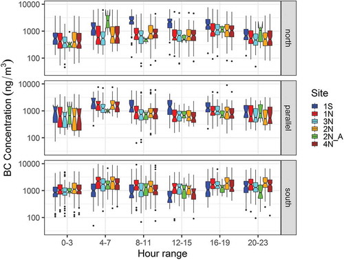
Figure 3. Campaign III gradients in hourly average binned BC concentrations (ng/m³) measured by microAeths when winds are from the north (top), parallel (middle), and south (bottom)

Mann-Whitney U-Tests were run on wind bin aggregated datasets from Campaigns I/II and III by site (i.e., not segregated by hour-range as shown in Figures 2 and 3) to determine whether the distributions of concentrations were statistically significant at the 95% confidence level. Note that the Mann-Whitney U-Test is non-parametric so does not assume anything about the shape of the concentration distribution. Concentration distributions at Site 1S were significantly higher than those at other sites farther from I-70 in both Campaigns I/II and Campaign III.

Gradients stratified by wind bins in the 120-degree arcs relative to the roadway were statistically significant across many of the comparisons in both the Campaign I/II and Campaign III datasets. When winds were perpendicular to I-70, statistically significant gradients of 500–800 ng/m³ were found at all downwind sites. The higher downwind concentrations cause higher exposures for people downwind of I-70 during those periods; BC was significantly higher than at upwind sites during these conditions.

Thus, we find that proximity to the highway is the most important contributor to exposure over long time periods, but wind direction relative to I-70 is the most important contributor for shorter-term exposure periods. These shorter-term exposure periods can be grouped into activity exposure periods to determine whether children attending elementary schools are downwind of I-70 during school hours, for example, and to assess whether their relative exposures will be higher than those of children attending nearby schools located farther from major roadways.

VOC sampling in Campaign III

In Campaign III, VOC samples were collected on 22 days. Individual samples from each site were compared to daily mean concentrations to determine the relative increments at each site. The average increments at individual sites were never statistically significantly larger than at other sites, largely as a result of large standard deviations in the population means. Supplemental Table 1 shows the summary statistics for all pollutants collected during Campaign III that had valid above-detection-limit samples with more than 75% of samples collected. Given that the sample size was only 22 days, the uncertainty in mean concentrations was larger than any concentration differences across sites. For example, the percentages of the standard deviations for most of the hydrocarbons (not the chlorofluorocarbons) were usually larger than 40%, resulting in 95% confidence intervals of around 20% for most site-pollutant means. When compared to 95% confidence intervals, all pollutants’ mean increments were statistically significantly indistinguishable from a mean value of 100%; i.e., none of the results are indicative of a population mean that is higher than the overall average with statistical significance. To detect gradients of less than 15% (i.e., the magnitude calculated for aggregated BC gradients) across sites with the temporal variability in concentrations that were observed day-to-day, at least 80 daily samples at each site would be needed to get confidence intervals down to the 10% level. Note: this does not imply that there is no gradient or that the gradient is ~15% across sites; we are simply stating that a gradient of less than 30% relative magnitude could not be detected with statistical confidence based on the limited number of samples, the uncertainty in the measurement method, and the shifting winds over a 24-hr period of sample collection.

Two independent methods were used to identify potential emissions sources influencing the near-road sites for VOCs. In the first, we used enrichment ratio plots. Enrichment ratio plots normalize concentrations of two pollutants on the x-axis and y-axis by dividing them by the concentration of a third pollutant; this method helps to remove some of the meteorological variability from the standard scatter plot of two pollutants. In the second method, positive matrix factorization (PMF) was run on the combined data from all sites for VOCs to identify “factors” that correspond to emissions sources with covariant pollutant concentrations.

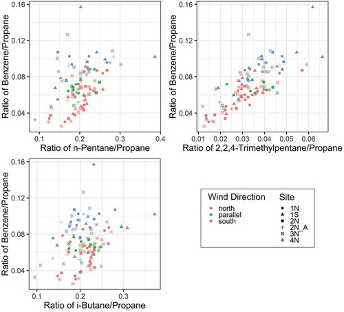
Enrichment ratio plots segregated by wind direction bin provide some evidence that multiple sources are affecting VOC concentrations at the near-road sites. Figure 4 shows the enrichment ratio plots for benzene and n-pentane divided by propane; benzene and 2,2,4-trimethlypentane divided by propane; and benzene and i-butane divided by propane. In the top left panel (benzene, n-pentane), the wind direction bins are clearly separated into a cluster of blue points indicating that higher ratios of benzene/propane occur when the wind blows from the south, whereas lower ratios of benzene/propane occur when the wind blows from the north. In contrast, in the top right panel, the relative ratios remain the same but the wind direction bins are aligned linearly. Finally, the bottom left panel shows benzene/propane and i-butane/propane; similar to n-pentane propane, the samples are clustered by wind direction with clear bifurcation of the patterns between southerly and northerly winds. The contrast between the three sets of figures clearly indicates a second hydrocarbon source in addition to mobile source emissions influencing the near-road sites.

Figure 4. Enrichment ratio scatter plots of (top, left) benzene and n-pentane divided by propane, (top, right) benzene and 2,2,4-trimethylpentane divided by propane, and (bottom, left) benzene and i-butane divided by propane. All figures are colored by wind direction bins, and sites are indicated by different shapes

Source apportionment using PMF on VOCs has been performed on data collected in areas such as Los Angeles, California; Houston, Texas; and Edmonton, Alberta (Brown, Frankel, and Hafner 2007; Buzcu and Fraser 2008; Field et al. 2015; McCarthy et al. 2013; Miller et al. 2002; Rappenglück et al. 2013; Watson, Chow, and Fujita 2001). PMF requires only ambient data, and assumptions regarding the numbers or types of sources or specific source profiles are not explicitly needed because PMF generates a set of factor profiles and contributions based on the input data and selected factor number (Brown et al. 2015; Paatero 1999). Multiple PMF scenarios were run to examine the potential number of emissions sources that could be identified using PMF. Scenarios were run with 3-, 4-, and 5-factor solutions. Initial runs that included isoprene always included a factor with isoprene as the dominant VOC, representing biogenic emissions. Isoprene was then excluded from the analysis because biogenic emissions sources were not of interest. In subsequent 3- and 4-factor runs, 3-factor solutions were as stable as 4-factor solutions with regard to bootstrapping (88% reproducibility for 3-factor solutions; 86% reproducibility for 4-factor solutions). These bootstrapping results are consistent with a relatively small matrix of total records (~120 samples and 50 species). The 3-factor solution results are classified in Table 5 and shown in Figure 5. Selecting a 4-factor solution split the mobile source factor into two separate categories with a long-chain alkane component with key tracers of n-decane and n-nonane; this may be representative of diesel exhaust emissions.

Table 5. Factors identified and key pollutants used to classify emissions sources in PMF

Factor	Factor Name	Key Pollutants in Factor
Factor 1	Mobile Source	Acetylene, ethene, toluene, 2,2,4-trimethylpentane, xylenes
Factor 2	Background	Carbon tetrachloride, Freons
Factor 3	Short-Chain Alkanes	Ethane, propane, n-butane, i-butane, n-pentane

Figure 5. Percent of pollutants identified in each factor with a 3-factor PMF solution excluding isoprene

Aldehyde sampling in Campaigns I and II

Daily carbonyl samples were collected over 36 days at six sites during Campaigns I and II. Analysis of the aggregate data showed that no gradients were statistically significant, with mean normalized site concentrations of formaldehyde and acetaldehyde varying by less than 15% across sites, significantly lower than the approximately 18-20% 95% confidence interval in the normalized mean. In other words, any gradients would not be statistically distinguishable unless they were much larger in magnitude than the small differences seen. To detect gradients of less than 15% across sites with the temporal variability in concentrations observed day-to-day, at least 120 daily samples at each site would be needed to get confidence intervals down to the 10% level. Daily concentration statistics for the carbonyls are provided in Supplemental Table 2.

AERMOD modeling results

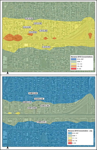
The AERMOD model was run separately for TAZ and link sources. The benzene concentrations from both models were then summed to calculated the predicted ambient benzene concentrations. Figure 6 (top) displays the spatial pattern of modeled benzene concentrations for the month of January in the study area. The exact model and monitor values are shown on the figure (shown as model(monitor)) and model to monitor ratios range from 0.83 to 1.38. Figure 6 (bottom) shows the model estimates of average benzene concentrations during the month of July as a representative of summer season. Model-to-monitor ratios range from 0.40 to 0.7 with most ratios less than a factor of 2. It is important to note that even though the benzene measurements were collected during September and October, comparison of these measurements with the model estimates of January and July showed good model performance. When applying what we know about meteorology and climatology by season/month in Denver, the modeled concentration for the Sep-Oct 2018 monitoring study would fall somewhere between January and July; midway would be a reasonable assumption. If that assumption is correct, then model-to-monitor ratios would range from 0.61 to 1.04, which would be considered excellent model performance. Overall, the model gradient (>0.5 ppb) in concentration is much larger than that observed in the measurements.

Figure 6. Predicted 24-hour averages of benzene concentrations during the month of January 2018 (top) or July 2018 (bottom) and the observed benzene measurements (24-hour averages) collected from September 15 through October 28, 2018. The values on the map are shown as: Model (Monitor)

Discussion

For this study, multiple temporary monitoring stations were deployed in the environmental justice community of Elyria-Swansea in the vicinity of Swansea Elementary School. Monitoring stations were within 200 m of I-70, a large freeway with AADT of 153,000 vehicles.

MicroAethalometer measurements of BC provided statistically significant concentration gradients for the near-road environment in the community. Over the three campaigns, under downwind conditions, hourly average BC concentrations at downwind sites were on the order of 500–800 ng/m³ higher than those upwind of I-70 during the same hours. This increment was 30-80% higher than average concentrations of BC upwind of I-70. However, aggregation of the concentrations over the entire campaign timeframe with winds alternating between upwind and downwind significantly reduced the total expected exposures of persons living or working next to I-70. Maximum increments observed at sites within 20 m of I-70 were 150–300 ng/m³ higher than those observed at sites 150 m from I-70 during the same time period. Aggregate increments were reduced relative to the wind-segregated bins due to the shifting winds relative to I-70’s east-west orientation. These total increments were only 11-18% higher than concentrations observed 100–150 m from I-70 under the same wind conditions. This apparent reduction may be an important consideration when modeling exposures and expected health impacts for persons living or working in the near-road environment.

In contrast to previous work in this area, we found that integrated gradients in concentrations in the near-road environment were relatively small. The classic work by Zhu et al. (2002a) showed an exponential decrease in roadway BC concentrations in Los Angeles, and many follow-up studies in the 2000s showed that BC gradients were large relative to background, i.e., > 80% (Woodruff et al. 1998). Saha et al. (2018b) show a BC gradient around 500–800 ng/m³ above background (400 m upwind site) in the wintertime, using measurements that are primarily downwind. This study found a comparable BC downwind gradient on the order of 500–800 ng/m³, relative to the upwind site (16 meters upwind). In contrast to the study by Saha et al. (2018b) this study found a small BC gradient of 150–300 ng/m³, over 150 meters from the roadway. This could be due to differences in dispersion related to wind speed in Denver, or because the sampling time of the measurements was integrated over longer periods for this study. While total upwind versus downwind gradients were as large as a 40% increment on the downwind side of the highway, the integrated gradients over all wind directions and samples were small, only 15%. This means that hours when receptors are downwind of a freeway BC concentrations are well above background, and that when integrated over multiple months, BC concentrations are 15% higher next to the freeway than at greater distances from the freeway. The smaller gradients observed here may be due to cleaner diesel vehicles resulting from tighter emissions standards as the vehicle fleet becomes cleaner over time. This is consistent with an overall observed decreasing trend in black carbon in near-road and urban settings (Dallmann and Harley 2010; McDonald et al. 2013; Milando, Huang, and Batterman 2016; Rattigan et al. 2013) Alternately, the smaller gradient may be due to the longer time period and integrated measurement relative to most shorter-term studies (Saha et al. 2018b), or it could be a local fleet with a younger age distribution than in other study locations. It is also possible that the emissions are a result of a shifting emissions profile, with lower black carbon emissions and higher amounts of other pollutants that were not measured in this study (e.g., ultrafines). Finally, the smaller gradient may be partly attributable to the elevated roadway configuration (Heist, Perry, and Brixey 2009; Steffens et al. 2014).

Following up on the BC comparison, the VOCs and carbonyls provided no quantitative gradients that could be significantly distinguished from the concentrations at other sites. While this may appear to be a null result, we can constrain the possible size of gradient that could be present given our confidence in our ability to measure the concentrations of the VOCs and carbonyls. Our typical 95% confidence intervals for the individual site-parameter combinations were on the order of ±20%. Propagating uncertainty across multiple sites, we can estimate that concentration gradients on the order of 29% would be theoretically detectable with a 95% confidence level. Note that the 29% value is derived from the comparison of two mean concentrations at two separate sites that each have an individual uncertainty of ±20%; the combined uncertainty is larger because the two means have independent uncertainties that are combined in quadrature. None of the individual sites or parameters displayed a 30% gradient in concentrations, as shown in the supplemental tables. Therefore, we can quantitatively state that if there are gradients in concentrations of these species in the near-road environment, they are smaller than 20% in magnitude, i.e., essentially as small as or smaller than the gradients in BC. In addition, we can state that with typical day-to-day variance in meteorology (wind speed and wind direction), we would need at least four times as many samples to theoretically quantify gradients on the order of 10% (similar to the size of the aggregated gradient observed for BC). This may be a useful guideline for future studies considering near-road gradient analyses.

Model performance was excellent in terms of all monitors predicting benzene concentrations at levels within a factor of two of observed measured concentrations. We note that the winds observed at the Rocky Mountain Arsenal site used for the modeling are significantly higher in speed than those observed at the Swansea monitoring site, and this may bias the model concentration estimates lower than what would be expected with wind speeds more characteristic of the urban area.

Conclusion

Air pollutant concentrations are often higher near major roadways than in the surrounding environment owing to the proximity of emissions from on-road mobile sources. In this study, we quantified the gradient in black carbon concentrations in the near-road environment of the Elyria-Swansea environmental justice neighborhood in Denver, Colorado. The gradient in concentrations segregated by wind direction from the roadway was 500–800 ng/m³, equal to an increment of approximately 30-80% above local background levels. When integrated over all wind directions, the gradients were smaller, approximately 150–300 ng/m³ (~11-18%) over the course of about four months of measurements. These gradient estimates are smaller than those found in previous studies and may be due to cleaner diesel vehicles complying with Tier 2 and 3 emissions standards.

Measurements of VOCs and carbonyls were unable to statistically quantify gradients because the gradients were too small in magnitude (<30%) compared to the number of samples and uncertainty in measurements. This finding is also in contrast to studies reported in Karner, Eisinger, and Niemeier (2010), but may be due to significant reductions in emissions over the past 10 to 20 years that result in a smaller near-road gradient over an urban background. We estimate that sample sizes of at least 100 individual measurements would have been required to estimate mean concentrations with sufficient certainty to quantify gradients on the order of 15%. These results suggest that recent decades of improved emissions standards and the steady turnover of the vehicle fleet may be reducing the impact of the roadway environment on near-road communities.

Disclosure statement

No potential conflict of interest was reported by the authors.

Supplementary material

The supplemental data for this article can be accessed on the publisher’s website.

Additional information

Funding

This work was supported by the Environmental Protection Agency [17 FAAA 93541].

Notes on contributors

Michael C. McCarthy

Michael C. McCarthy and Anondo D. Mukherjee are Atmospheric Scientists at Sonoma Technology, Inc. (STI), located in Petaluma, California

Michael Ogletree

Michael Ogletree is an Air Quality Program Manager at the Denver Department of Public Health & Environment in Denver, Colorado.

Jonathan Furst

Jonathan Furst and Marie I. Gosselin are Field Specialists at Air Resource Specialists

Mark Tigges

Mark Tigges is a Program Manager at Air Resource Specialists, located in Fort Collins, Colorado.

Gregg Thomas

Gregg Thomas is the Environmental Quality Division Director at the Denver Department of Public Health & Environment.

Steven G. Brown

Steven G. Brown is a Vice President of STI and Manager of the Data Science Department.

References

- Apelberg, B. J., T. J. Buckley, and R. H. White. 2005. Socioeconomic and racial disparities in cancer risk from air toxics in Maryland. Environ. Health Perspect. 113 (6):693–99. doi:10.1289/ehp.7609.
- Baldauf, R., E. Thoma, M. Hays, R. Shores, J. S. Kinsey, B. Gullet, S. Kimbrough, V. Isakov, T. Long, R. Snow, et al. 2008. Traffic and meteorological impacts on near-road air quality: Summary of methods and trends from the Raleigh near-road study. J. Air Waste Manage. Assoc. 58:865–78. doi:10.3155/1047-3289.58.7.865.
- Barzyk, T. M., V. Isakov, S. Arunachalam, A. Venkatram, R. Cook, and B. Naess. 2015. A near-road modeling system for community-scale assessments of traffic-related air pollution in the United States. Environ. Modell. Softw. 66:46–56. doi:10.1016/j.envsoft.2014.12.004.
- Bates, J. T., A. F. Pennington, X. Zhai, M. D. Friberg, F. Metcalf, L. Darrow, M. Strickland, J. Mulholland, and A. Russell. 2018. Application and evaluation of two model fusion approaches to obtain ambient air pollutant concentrations at a fine spatial resolution (250m) in Atlanta. Environ. Modell. Softw. 109:182–90. doi:10.1016/j.envsoft.2018.06.008.
- Brandt, S., L. Perez, N. Künzli, F. Lurmann, J. Wilson, M. Pastor, and R. McConnell. 2014. Cost of near-roadway and regional air pollution–attributable childhood asthma in Los Angeles County. J. Allergy Clin. Immunol. 134 (5):1028–35. doi:10.1016/j.jaci.2014.09.029.
- Brown, S. G., S. Eberly, P. Paatero, and G. A. Norris. 2015. Methods for estimating uncertainty in PMF solutions: Examples with ambient air and water quality data and guidance on reporting PMF results. Sci. Total Environ. 518-519:626–35. doi:10.1016/j.scitotenv.2015.01.022.
- Brown, S. G., A. Frankel, and H. R. Hafner. 2007. Source apportionment of VOCs in the Los Angeles area using positive matrix factorization. Atmos. Environ. 41:227–237.STI-2725. doi:10.1016/j.atmosenv.2006.08.021.
- Brown, S. G., M. C. McCarthy, J. L. DeWinter, D. L. Vaughn, and P. T. Roberts. 2014. Changes in air quality at near-roadway schools after a major freeway expansion in Las Vegas, Nevada. J. Air Waste Manage. Assoc. 64(9):1002–12. STI-3889. doi:10.1080/10962247.2014.907217.
- Brugge, D., J. L. Durant, and C. Rioux. 2007. Near-highway pollutants in motor vehicle exhaust: A review of epidemiologic evidence of cardiac and pulmonary health risks. Environ. Health 6 (23). doi:10.1186/1476-069X-6-23.
- Buzcu, B., and M. P. Fraser. 2008. Comparison of VOC emissions inventory data with source apportionment results for Houston, TX. Atmos. Environ. 42:5032–43. doi:10.1016/j.atmosenv.2008.02.025.
- Cai, J., B. Yan, J. Ross, D. Zhang, P. L. Kinney, M. S. Perzanowski, K. Jung, R. Miller, and S. N. Chillrud. 2014. Validation of MicroAeth® as a black carbon monitor for fixed-site measurement and optimization for personal exposure characterization. Aerosol. Air Quality Res. 14 (1):1–9. doi:10.4209/aaqr.2013.03.0088.
- Chang, S. Y., W. Vizuete, M. Breen, V. Isakov, and S. Arunachalam. 2015. Comparison of highly resolved model-based exposure metrics for traffic-related air pollutants to support environmental health studies. Int. J. Environ. Res. Public Health 12 (12):15605–25. doi:10.3390/ijerph121215007.
- Cheng, Y.-H., and M.-H. Lin. 2013. Real-time performance of the microAeth® AE51 and the effects of aerosol loading on its measurement results at a traffic site. Aerosol. Air Quality Res. 13 (6):1853–63. doi:10.4209/aaqr.2012.12.0371.
- Clark-Reyna, S. E., S. E. Grineski, and T. W. Collins. 2016. Health status and residential exposure to air toxics: What are the effects on children’s academic achievement? Fam. Community Health 39 (3):160–68. doi:10.1097/fch.0000000000000112.
- Dallmann, T., S. DeMartini, T. Kirchstetter, S. Herndon, and T. Onasch. 2012. On-road measurement of gas and particle phase pollutant emission factors for individual heavy-duty diesel trucks. Environ. Sci. Technol. 46 (15):8511–18. doi:10.1021/es301936c.
- Dallmann, T. R., and R. A. Harley. 2010. Evaluation of mobile source emission trends in the United States. J Geophys. Res. Atmos. 115. doi:10.1029/2010jd013862.
- Field, R. A., J. Soltis, M. C. McCarthy, S. Murphy, and D. C. Montague. 2015. Influence of oil and gas field operations on spatial and temporal distributions of atmospheric non-methane hydrocarbons and their effect on ozone formation in winter. Atmos. Chem. Phys. 15:3527–42. STI-6271. doi:10.5194/acp-15-3527-2015.
- Fruin, S. A., M. J. St. Denis, A. M. Winer, S. D. Colome, and F. W. Lurmann. 2001. Reductions in human benzene exposure in the California South Coast Air Basin. Atmos. Environ. 35:1069–77. doi:10.1016/S1352-2310(00)00306-X.
- Ghosh, R., W. J. Gauderman, H. Minor, H. A. Youn, F. Lurmann, K. R. Cromar, L. Chatzi, B. Belcher, C. R. Fielding, and R. McConnell. 2017. Air pollution, weight loss and metabolic benefits of bariatric surgery: A potential model for study of metabolic effects of environmental exposures. Pediatr. Obes. doi:10.1111/ijpo.12210.
- Ghosh, R., F. Lurmann, L. Perez, B. Penfold, S. Brandt, J. Wilson, M. Milet, N. Künzli, and R. McConnell. 2016. Near-roadway air pollution and coronary heart disease: Burden of disease and potential impact of greenhouse gas reduction strategy in southern California. Environ. Health Perspect. 124 (2):193–200. doi:10.1289/ehp.1408865.
- Ginzburg, H., X. Liu, M. Baker, R. Shreeve, R. K. M. Jayanty, D. Campbell, and B. Zielinska. 2015. Monitoring study of the near-road PM2.5 concentrations in Maryland. J. Air Waste Manage. Assoc. 65 (9):1062–71. doi:10.1080/10962247.2015.1056887.
- Hagler, G. S. W., R. W. Baldauf, E. D. Thoma, T. R. Long, R. F. Snow, J. S. Kinsey, L. Oudejans, and B. K. Gullett. 2009. Ultrafine particles near a major roadway in Raleigh, North Carolina: Downwind attenuation and correlation with traffic-related pollutants. Atmos. Environ. 43:1229–34. doi:10.1016/j.atmosenv.2008.11.024.
- Health Effects Institute. 2010. Traffic-related air pollution: A critical review of the literature on emissions, exposure, and health effects. Special Report 17, Report prepared by the Health Effects Institute, Boston, MA, January. https://www.healtheffects.org/publication/traffic-related-air-pollution-critical-review-literature-emissions-exposure-and-health.
- Health Effects Institute Air Toxics Review Panel. 2007. Mobile-source air toxics: A critical review of the literature on exposure and health effects. Special Report 16, Prepared by the Health Effects Insitute, Boston, MA, November.
- Heist, D. K., S. G. Perry, and L. A. Brixey. 2009. A wind tunnel study of the effect of roadway configurations on the dispersion of traffic-related pollution. Atmos. Environ. 43:5101–11. doi:10.1016/j.atmosenv.2009.06.034.
- Houston, D., M. Krudysz, and A. Winer. 2008. Diesel truck traffic in port-adjacent low income and minority communities; environmental justice implications of near roadway land use conflicts. Transp. Res. Rec. 2076:38–46. doi:10.3141/2067-05.
- Jeong, C.-H., J. M. Wang, N. Hilker, J. Debosz, U. Sofowote, Y. Su, M. Noble, R. M. Healy, T. Munoz, E. Dabek-Zlotorzynska, et al. 2019. Temporal and spatial variability of traffic-related PM2.5 sources: Comparison of exhaust and non-exhaust emissions. Atmos. Environ. 198:55–69. doi:10.1016/j.atmosenv.2018.10.038.
- Karner, A., D. S. Eisinger, and D. Niemeier. 2010. Near-roadway air quality: Synthesizing the findings from real-world data. Environ. Sci. Technol. 44:5334–5344. STI-3923. doi:10.1021/es100008x.
- Kirchstetter, T. W., and T. Novakov. 2007. Controlled generation of black carbon particles from a diffusion flame and applications in evaluating black carbon measurement methods. Atmos. Environ. 41 (9):1874–88. doi:10.1016/j.atmosenv.2006.10.067.
- Kleeman, M. J., S. G. Riddle, M. A. Robert, C. A. Jakober, P. M. Fine, M. D. Hays, J. J. Schauer, and M. P. Hannigan. 2009. Source apportionment of fine (PM1.8) and ultrafine (PM0.1) airborne particulate matter during a severe winter pollution episode. Environ. Sci. Technol. 43 (2):272–79. doi:10.1021/es800400m.
- Loh, M. M., J. I. Levy, J. D. Spengler, E. A. Houseman, and D. H. Bennett. 2007. Ranking cancer risks of organic hazardous air pollutants in the United States. Environ. Health Perspect. 115 (8):1160–68. doi:10.1289/ehp.9884.
- Lovinsky-Desir, S., J. Lawrence, K. H. Jung, A. G. Rundle, L. A. Hoepner, B. Yan, F. Perera, M. S. Perzanowski, R. L. Miller, and S. N. Chillrud. 2018. Assessment of exposure to air pollution in children: Determining whether wearing a personal monitor affects physical activity. Environ. Res. 166:340–43. doi:10.1016/j.envres.2018.06.017.
- McCarthy, M. C., Y.-A. Aklilu, S. G. Brown, and D. A. Lyder. 2013. Source apportionment of volatile organic compounds measured in Edmonton, Alberta. Atmos. Environ. 81:504–516.STI-5652. doi:10.1016/j.atmosenv.2013.09.016.
- McDonald, B. C., D. R. Gentner, A. H. Goldstein, and R. A. Harley. 2013. Long-term trends in motor vehicle emissions in U.S. urban areas. Environ. Sci. Technol. 47 (17):10022–31. doi:10.1021/es401034z.
- Milando, C., L. Huang, and S. Batterman. 2016. Trends in PM2.5 emissions, concentrations and apportionments in Detroit and Chicago. Atmos. Environ. 129:197–209. doi:10.1016/j.atmosenv.2016.01.012.
- Miller, S. L., M. J. Anderson, E. P. Daly, and J. B. Milford. 2002. Source apportionment of exposures to volatile organic compounds. I. Evaluation of receptor models using simulated exposure data. Atmos. Environ. 36 (22):3628–41. doi:10.1016/S1352-2310(02)00279-0.
- Miranda, M. L., S. E. Edwards, M. H. Keating, and C. J. Paul. 2011. Making the environmental justice grade: The relative burden of air pollution exposure in the United States. Int. J. Environ. Res. Public Health 8 (6):1755–71. doi:10.3390/ijerph8061755.
- Morello-Frosch, R., and E. D. Shenassa. 2006. The environmental “riskscape” and social inequality: Implications for explaining maternal and child health disparities. Environ. Health Perspect. 114 (8):1150–53. doi:10.1289/ehp.8930.
- Oakes, M. M., J. M. Burke, G. A. Norris, K. D. Kovalcik, J. P. Pancras, and M. S. Landis. 2016. Near-road enhancement and solubility of fine and coarse particulate matter trace elements near a major interstate in Detroit, Michigan. Atmos. Environ. 145:213–24. doi:10.1016/j.atmosenv.2016.09.034.
- Paatero, P. 1999. The multilinear engine - A table-driven, least squares program for solving multilinear problems, including the n-way parallel factor analysis model. J. Graph. Statist. 8:854–88.
- Parvez, F., and K. Wagstrom. 2019. A hybrid modeling framework to estimate pollutant concentrations and exposures in near road environments. Sci. Total Environ. 663:144–53. doi:10.1016/j.scitotenv.2019.01.218.
- Patterson, R. F., and R. A. Harley. 2019. Evaluating near-roadway concentrations of diesel-related air pollution using RLINE. Atmos. Environ. 199:244–51. doi:10.1016/j.atmosenv.2018.11.016.
- Pope, C. A., and D. W. Dockery. 2006. Health effects of fine particulate air pollution: Lines that connect. J. Air Waste Manage. Assoc. 56:709–42. doi:10.1080/10473289.2006.10464485.
- Rappenglück, B., G. Lubertino, S. Alvarez, J. Golovko, B. Czader, and L. Ackermann. 2013. Radical precursors and related species from traffic as observed and modeled at an urban highway junction. J. Air Waste Manage. Assoc. 63 (11):1270–86. doi:10.1080/10962247.2013.822438.
- Rattigan, O. V., K. Civerolo, P. Doraiswamy, H. D. Felton, and P. K. Hopke. 2013. Long term black carbon measurements at two urban locations in New York. Aerosol Air Qual. Res 13 (4):1181–96. doi:10.4209/aaqr.2013.02.0060.
- Reid, S., S. Bai, Y. Du, K. Craig, G. Erdakos, L. Baringer, D. Eisinger, M. McCarthy, and K. Landsberg. 2016. Emissions modeling with MOVES and EMFAC to assess the potential for a transportation project to create particulate matter hot spots. Transp. Res. Rec. 2570:12–20. STI-6330. doi:10.3141/2570-02.
- Riddle, S. G., M. A. Robert, C. A. Jakober, M. P. Hannigan, and M. J. Kleeman. 2008. Size-resolved source apportionment of airborne particle mass in a roadside environment. Environ. Sci. Technol. 42 (17):6580–86. doi:10.1021/es702827h.
- Riley, E. A., L. Banks, J. Fintzi, T. R. Gould, K. Hartin, L. Schaal, M. Davey, L. Sheppard, T. Larson, M. G. Yost, et al. 2014. Multi-pollutant mobile platform measurements of air pollutants adjacent to a major roadway. Atmos. Environ. 98:492–99. doi:10.1016/j.atmosenv.2014.09.018.
- Rivas, I., D. Donaire-Gonzalez, L. Bouso, M. Esnaola, M. Pandolfi, M. de Castro, M. Viana, M. Àlvarez-Pedrerol, M. Nieuwenhuijsen, A. Alastuey, et al. 2016. Spatiotemporally resolved black carbon concentration, schoolchildren’s exposure and dose in Barcelona. Indoor Air 26 (3):391–402. doi:10.1111/ina.12214.
- Rosenbaum, A. S., D. A. Axelrad, T. J. Woodruff, Y. H. Wei, M. P. Ligocki, and J. P. Cohen. 1999. National estimates of outdoor air toxics concentrations. J. Air Waste Manage. Assoc. 49 (10):1138–52. doi:10.1080/10473289.1999.10463919.
- Rowangould, G. M. 2013. A census of the US near-roadway population: Public health and environmental justice considerations. Transp. Res. Part D Transport Environ. 25:59–67. doi:10.1016/j.trd.2013.08.003.
- Saha, P. K., A. Khlystov, and A. P. Grieshop. 2018a. Downwind evolution of the volatility and mixing state of near-road aerosols near a US interstate highway. Atmos. Chem. Phys. 18 (3):2139–54. doi:10.5194/acp-18-2139-2018.
- Saha, P. K., A. Khlystov, M. G. Snyder, and A. P. Grieshop. 2018b. Characterization of air pollutant concentrations, fleet emission factors, and dispersion near a North Carolina interstate freeway across two seasons. Atmos. Environ. 177:143–53. doi:10.1016/j.atmosenv.2018.01.019.
- Skov, H., A. B. Hansen, G. Lorenzen, H. V. Andersen, P. Lofstrom, and C. S. Christensen. 2001. Benzene exposure and the effect of traffic pollution in Copenhagen, Denmark. Atmos. Environ. 35 (14):2463–71. doi:10.1016/S1352-2310(00)00460-X.
- Smith, M. T. 2010. Advances in understanding benzene health effects and susceptibility. Annu. Rev. Public Health 31 (1):133–48. doi:10.1146/annurev.publhealth.012809.103646.
- Steffens, J., D. Heist, S. Perry, V. Isakov, R. Baldauf, and K. M. Zhang. 2014. Effects of roadway configurations on near-road air quality and the implications on roadway designs. Atmos. Environ. 94:74–85. doi:10.1016/j.atmosenv.2014.05.015.
- Thomas, G. W., M. Ogletree, and L. Clay. 2016. Going one step beyond in North Denver, a neighborhood scale air pollution modeling assessment, Part II: Predicted ambient concentrations in 2035. Colorado Department of Transportation. https://www.codot.gov/programs/research/pdfs/2007/goodneighbor.pdf.
- Thomas, G. W., S. M. Williams, and D. L. Bain. 2007. Going one step beyond: A neighborhood scale air toxics assessment in north Denver (the Good Neighbor Project). Technical report prepared for the The Colorado Department of Transportation, Denver, CO, and the Federal Highway Administration, Colorado Division, Lakewood, CO, by the City and County of Denver Department of Environmental Health, March 9.
- U.S. Environmental Protection Agency. 1996. Guidelines for carcinogen risk assessment. Washington, DC: U.S. EPA.
- U.S. Environmental Protection Agency. 1999a. Compendium of methods for the determination of toxic organic compounds in ambient air: Compendium method TO-11A. 2nd ed. Cincinnati, OH: prepared by the U.S. Environmental Protection Agency, Office of Research and Development. EPA/625/R-96/010b, January. https://www3.epa.gov/ttnamti1/files/ambient/airtox/to-11ar.pdf.
- U.S. Environmental Protection Agency. 1999b. Compendium of methods for the determination of toxic organic compounds in ambient air: Compendium method TO-15. 2nd ed. Cincinnati, OH: prepared by the U.S. Environmental Protection Agency, Office of Research and Development. EPA/625/R-96/010b, January. https://www3.epa.gov/ttnamti1/files/ambient/airtox/tocomp99.pdf.
- U.S. Environmental Protection Agency. 2000. Control of air pollution from new motor vehicles: Tier 2 motor vehicle emissions standards and gasoline sulfur control requirements. Fed. Regist. 65 (28):6698–822. Final rule, 40 CFR Parts 80, 85, and 86, February 10. http://www.epa.gov/otaq/regs/ld-hwy/tier-2/frm/fr-t2pre.pdf.
- U.S. Environmental Protection Agency. 2007. Control of hazardous air pollutants from mobile sources, Chapter 3: Air quality and resulting health and welfare effects of air pollution from mobile sources. Regulatory impact analysis prepared by the Assessment and Standards Division, Office of Transportation and Air Quality, U.S. Environmental Protection Agency, Research Triangle Park, NC, EPA420-R-07-002, February.
- U.S. Environmental Protection Agency. 2014a. Control of air pollution from motor vehicles: Tier 3 motor vehicle emission and fuel standards. 79 Fed. Regist. 81:23414–886. https://www.epa.gov/regulations-emissions-vehicles-and-engines/final-rule-control-air-pollution-motor-vehicles-tier-3#rule-history.
- U.S. Environmental Protection Agency. 2014b. National air toxics program: the second integrated urban air toxics report to Congress. August 21. https://www2.epa.gov/sites/production/files/2014-08/documents/082114-urban-air-toxics-report-congress.pdf.
- U.S. Environmental Protection Agency. 2015a. 2011 National Air Toxics Assessment (NATA). December 17. https://www.epa.gov/national-air-toxics-assessment.
- U.S. Environmental Protection Agency. 2015b. MOVES2014 and MOVES2014a technical guidance: Using MOVES to prepare emission inventories for state implementation plans and transportation conformity. EPA-420-B-15-093, November. http://www3.epa.gov/otaq/models/moves/documents/420b15093.pdf.
- U.S. Environmental Protection Agency. 2016. Air toxic emissions from on-road vehicles in MOVES2014. EPA-420-R-16-016, November. https://nepis.epa.gov/Exe/ZyPDF.cgi?Dockey=P100PUNO.pdf.
- U.S. Environmental Protection Agency. 2017. EJSCREEN environmental justice mapping and screening tool: Technical documentation. August. https://www.epa.gov/ejscreen.
- U.S. Environmental Protection Agency. 2018. Technical support document: EPA’s 2014 National Air Toxics Assessment. 2014 NATA TSD, August.
- U.S. Environmental Protection Agency. 2019. Our nation’s air: Status and trends through 2018. https://gispub.epa.gov/air/trendsreport/2019.
- Urman, R., R. McConnell, T. S. Islam, E. L. Avol, F. W. Lurmann, H. Vora, W. S. Lin, E. B. Rappaport, F. D. Gilliland, and W. J. Gauderman. 2014. Associations of children’s lung function with ambient air pollution: Joint effects of regional and near-roadway pollutants. Thorax 69 (6):540–47. doi:10.1136/thoraxjnl-2012-203159.
- Viana, M., I. Rivas, C. Reche, A. S. Fonseca, N. Pérez, X. Querol, A. Alastuey, M. Álvarez-Pedrerol, and J. Sunyer. 2015. Field comparison of portable and stationary instruments for outdoor urban air exposure assessments. Atmos. Environ. 123:220–28. doi:10.1016/j.atmosenv.2015.10.076.
- Watson, J. G., J. C. Chow, and E. M. Fujita. 2001. Review of volatile organic compound source apportionment by chemical mass balance. Atmos. Environ. 35:1567–84. doi:10.1016/S1352-2310(00)00461-1.
- Wilhelm, M., J. K. Ghosh, J. Su, M. Cockburn, M. Jerrett, and B. Ritz. 2011. Traffic-related air toxics and preterm birth: A population-based case-control study in Los Angeles County, California. Environ. Health 10 (89). doi:10.1186/1476-069X-10-89.
- Woodruff, T. J., D. A. Axelrad, J. Caldwell, R. Morello-Frosch, and A. Rosenbaum. 1998. Public health implications of 1990 air toxics concentrations across the United States. Environ. Health Perspect. 106 (5):245–51. doi:10.1289/ehp.98106245.
- Woodruff, T. J., J. Caldwell, V. J. Cogliano, and D. A. Axelrad. 2000. Estimating cancer risk from outdoor concentrations of hazardous air pollutants in 1990. Environ. Res. 82 (3):194–206. doi:10.1006/enrs.1999.4021.
- Zhu, Y., W. C. Hinds, S. Kim, S. Shen, and C. Sioutas. 2002a. Study of ultrafine particles near a major highway with heavy-duty diesel traffic. Atmos. Environ. 36 (27):4323–35. doi:10.1016/s1352-2310(02)00354-0.
- Zhu, Y. F., W. C. Hinds, S. Kim, and C. Sioutas. 2002b. Concentration and size distribution of ultrafine particles near a major highway. J. Air Waste Manage. Assoc. 52 (9):1032–42. doi:10.1080/10473289.2002.10470842.
- Zhu, Y. F., W. C. Hinds, S. Shen, and C. Sioutas. 2004. Seasonal trends of concentration and size distribution of ultrafine particles near major highways in Los Angeles. Aerosol Sci. Technol. 38:5–13. doi:10.1080/02786820390229156.