Quantification of gasoline-ethanol blend emissions effects

ABSTRACT

Emissions levels from current gasoline spark-ignited engines are low, and emissions changes associated with the blending of ethanol into gasoline are small and difficult to quantify. Addition of ethanol, with a high blending octane number, allows a reduction in aromatics in market gasoline. Blending behavior of ethanol is nonlinear, altering the distillation curve, including the 50% temperature point, T50. Increase in gasoline direct injection (GDI) engine technology in the fleet challenges ability of older models based on port fuel injection (PFI) results to predict the overall air quality impact of ethanol blending. Five different models derived from data collected through U.S. Environmental Protection Agency Energy Policy Act (EPAct) programs were used to predict LA92 Phase 1 particulate matter (PM) emissions for summer regular (SR) E0 (gasoline with 0% ethanol by volume), E10 (gasoline with 10% ethanol) and E15 (gasoline with 15% ethanol). Substantial reductions of PM for E10 and E15 relative to E0 were predicted when aromatics were displaced by ethanol to maintain octane rating. SR E0 and E10 were also matched to linear combinations of EPAct fuels and results showed a 35% PM reduction for SR E10 relative to SR E0. For GDI vehicles the Coordinating Research Council (CRC) E-94-3 study found that E10 had 23% or 29% PM increase. However, CRC E-129 found an E10 PM reduction of 10% when one E0 fuel and its splash blended (SB) E10 were compared. Both CRC project E-129 SB data and fuel triplets selected from the EPAct study showed variation for E15 emissions, although E-129 suggests that E15 in GDI offers about a 25% reduction of PM with respect to E0. Overall, data suggest that ethanol blending offers a modest to a substantial reduction of cold-start PM mass if aromatic levels of the finished products are reduced in response to ethanol addition.

Implications: Studies of exhaust emissions effects of ethanol blending with gasoline vary in conclusions. Blending properties are nonlinear. Modeling of real-world emissions effects must consider all fuel composition adjustments and property changes associated with ethanol addition. Aromatics are reduced in E10 or E15, compared with E0, and distillation changes. PFI-derived models show reductions in cold-start PM for expected average E10 versus E0 pump fuel, due to reduced aromatic content. Relative emissions effects from older technology (PFI) engines do not predict newer engine (GDI) results reliably, but recent GDI data show reduced cold-start PM when ethanol displaces aromatics.

Introduction

Ethanol use in gasoline

The ability of a spark-ignited engine fuel to resist knock is a desirable property because it allows the operation of a more efficient engine with a higher compression ratio or intake boost. Methyl Tertiary-Butyl Ether (MTBE) was employed as a gasoline additive in the USA from 1979 onwards as an octane rating enhancer to replace tetra-ethyl lead and to satisfy the federal requirement for oxygenates in reformulated gasoline (RFG). Subsequently, concern arose over the health effects of MTBE. The Environmental Protection Agency (EPA) appointed a Blue Ribbon Panel (EPA 2019) to examine the matter, and by 2000 five states had moved to curtail MTBE use. In 2005, the renewable fuel standard (RFS) paved the way for the blending of ethanol with a petroleum blendstock for oxygenate blending (BOB), for commercial sale. Between 2006 and this time of writing, a 10% (by volume) ethanol blend, E10, has been adopted widely. Ethanol shows a blending octane number that varies with the hydrocarbon composition but is considered to be over 110 AKI (anti-knock index: the average of Research Octane Number, RON, and Motor Octane Number, MON). Aromatics in market gasoline are a major contributor to raising AKI, but also represent a health concern: for example, benzene, toluene, ethyl benzene, and xylene (BTEX) pose significant health risks (Bolden, Kwiatkowski, and Colborn 2015) and are listed as hazardous air pollutants under the Clean Air Act (42U.S.C § 85 2013). BTEX toxicities have also been addressed separately in four papers (Fishbein 1984, 1985a, 1985b, 1985c). Fewer sources discuss health effects for aromatics other than BTEX present in gasoline. Aromatic health effects have been reviewed in a paper addressing solvents and European chemical control regulation requirements (McKee et al. 2018). The EPA presents information on naphthalene, though not from gasoline sources, and concludes that precise health effects are not available for propylbenzene (EPA 1998, 2009).

Premium and regular anti-knock ratings have been held constant over the last two decades, but the blending of ethanol allowed the octane ratings to be attained with the use of fewer aromatics and olefins in market gasoline, as shown in Figure 1.

Figure 1. Changes in the composition of gasoline over the period of ethanol introduction (EPA 2017). Aromatics reporting is addressed in 40 CFR Part 80.46 (f)(1) and (f)(3)

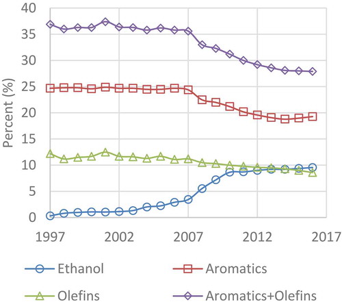
In 2006, average US gasoline contained 24.7% aromatics, 11.1% olefins, and 2.91% ethanol. In 2016 ethanol increased by 6.66% with a 5.4% reduction of aromatics and a 2.5% reduction in olefins. However, the ethanol and aromatics tradeoff in Figure 1 also represents the effect of other factors, such as increased demand for heavy components for diesel blending, changes in exports and premium fuel demand, and the sympathetic reduction of sulfur, benzene, MTBE, and olefins in gasoline. Data in the 2006–2016 EPA Fuel Trends Report show high variability in aromatic content both between refineries and overtime for individual refineries.

In 2012, the EPA approved the use of E15 for recent model-year vehicles, and this is now available widely, with the potential to reduce aromatic content further (EIA 2019).

Although U.S. light-duty vehicles are held to emissions standards while burning a defined certification fuel, it is widely recognized that the in-use fuel composition will have an effect on tailpipe emissions, and hence air quality. This paper summarizes major studies (Durbin et al. 2006; EPA 2013a, 2013b; Morgan et al. 2018, 2017; Schuchmann and Crawford 2019; Whitney 2014, Yang et al. 2019a) of ethanol blend effects on light-duty vehicle tailpipe emissions, presents the complexity of emissions prediction, and predicts the emissions from market gasoline using models derived from EPAct study data. Modeling and measured PM data for the E-94-2 (Morgan et al. 2017), E-94-3 (Morgan et al. 2018) and E-129 (Schuchmann and Crawford 2019) studies are also compared to EPAct reduction predictions to examine changes arising from the adoption of GDI technology. Data for E15 are contrasted with E10 and E0 at a time when mid blends are being more widely adopted (Guthrie 2015).

Air quality impacts

Vehicle tailpipe emissions contribute to regional inventories and impact air quality. Emissions of concern include oxides of nitrogen (NOx), carbon monoxide (CO), particulate matter by mass (PM), total hydrocarbons (HC), and non-methane organic gases (NMOG). In the USA, and in most other nations, emissions standards have been tightened over the last two decades, driving automotive technology change. The U.S. light-duty fleet has an average age of about 11 years, leading to a wide span of emissions levels and engine technologies for cars and light trucks in use. Therefore, older studies will report higher distance specific mass emissions than newer studies. However, it is not clear whether the relative emissions effects (as a percentage or ratio) for different levels of ethanol content may remain similar.

The majority of light-duty vehicles in the U.S. fleet use PFI. Driven by efficiency demands and GHG policy, in the last decade, there has been a revolutionary change with increased U.S. sales (now about 50%) of high-pressure gasoline direct injection (GDI) engines. Turbocharging grants GDI engines increased power density. They enjoy superior air/fuel ratio control, and they are usually downsized in displacement relative to PFI engines (Isenstadt et al. 2016). For GDI, PM emissions are of concern, being substantially higher than for PFI engines (Saliba et al. 2017; Zhang and McMahon 2012; Zhu et al. 2016). Fuel effects on PM emissions from GDI are therefore of elevated concern and are emphasized in this paper. NOx, as an ozone precursor, is also addressed.

There is growing interest in using higher octane blends to enable further efficiency gains with GDI technology (Leone et al. 2015). Ethanol may play a role in producing such blends. Generally, emissions from current production gasoline vehicles are very low. Typically emissions are higher for cold-start tests than for hot-stabilized tests where the catalyst is active throughout the vehicle operation.

Quantifying market fuel emissions effects

Studies that compare two or more fuels with different ethanol levels but with arbitrary petroleum content are unrepresentative of the market fuel composition. There are two productive pathways for comparing market gasoline emissions effects of a change of fuel specifications, from “A” to “B.” In both cases, the relevant fuel compositions must be identified.

First, in a pairwise study, one must identify the relevant fuel compositions first. Comprehensive fuel compositions that would represent Fuel A and Fuel B in the marketplace would be used for the emissions measurement. Market fuels that differ in ethanol content also differ in other properties, driven by regulation or economics or blending effects. Typically, an ethanol blend employs a refinery BOB that is formulated such that the final product, after blending with ethanol at a terminal, meets desired specifications at a competitive cost. If it is believed that Fuel A and Fuel B may each have a range of compositions in the marketplace, there could be more than one Fuel A and more than one Fuel B employed to quantify the range of relative emissions effects. Determining the composition of a BOB for large-scale future change is challenging, but composition must also be determined to predict emissions difference using a multivariate study model, as discussed below.

Second, one may perform a multivariate study, where the effects of several relevant fuel properties (one of which would be ethanol content) are examined, and employ statistical methods to create a predictive emissions model. This model can then be applied to the compositions of Fuels A and B to predict the effects of the change. The multivariate study is more expensive insofar as it seeks more information and examines more dimensions than a comparative study. Some of the information gained may not be useful in examining just the Fuel A to Fuel B change effects but the multivariate study can answer additional questions about property effects other than those associated with the A to B market composition change. Applicability of the multivariate model to A and B comparison will depend on the relevance of the study fuels and representativeness of the study variables. Nonlinear properties of blending may affect conclusions if orthogonality of study variables is assumed. Extrapolation of results to predict emissions from “unseen” blends outside the original experimental envelope will vary in reliability.

Gasoline emissions effects are usually examined on the basis of fuel descriptors, such as component fractions [e.g. PIANO analysis (Ratcliff et al. 2016)], properties [e.g. Research Octane Number (RON)] or parameters [e.g. distillation values]. These descriptors vary in their ability to identify the detailed composition of the fuel and to address processes occurring in the modern engine. Blending effects and properties may differ substantially between the liquid and vapor phases of the fuel, and between chemical and physical properties of the fuel. As an example, Kar et al. (2008) found that vaporization enthalpy for gasoline-ethanol mixtures varied in a curious fashion as the ethanol percentage rose. The mechanisms that cause fuel descriptors to affect emissions are complex, vary with engine speed, load and temperature history, and surely affect PFI and GDI engines (with varied control strategies) in different ways. Leone et al. (2015) questioned the applicability of the CFR engine used to determine the octane rating to modern engine designs.

Computed parameters, such as the Particulate Matter Index (PMI) (Aikawa, Sakurai, and Jetter 2010; Chapman et al. 2016) serve to condense detailed hydrocarbon analysis (DHA) (e.g. ASTM D6729) and are used as blending targets and study variables. However, such indices may not anticipate the complexity and variety of fuel composition and engine technology effects (Kalghatgi and Stone 2017; Sakai and Rothamer 2019).

Prior emissions studies

Prior studies of ethanol effects

Most studies of gasoline-ethanol effects have not employed market gasoline to determine ethanol blending emissions effects. Rather, they have either splash-blended ethanol into a candidate E0 gasoline or have prepared match blends (MB) that target certain parameters for a multivariate analysis. Major studies include CRC E-67 (MB) and E-94-2 (MB), E-94-3 (SB) and E-129 (SB) studies, the EPAct study (MB), a study for Growth Energy by the University of California, Riverside, and studies by the U.S. Department of Energy national laboratories. Numerous smaller studies have been conducted by academia, industry, and government. The CRC E-129 study (SB) has recently presented new GDI data. Further, GDI data using E0, E10, E15, and E20 have been presented recently by Yang et al. (2019a, 2019b). Details of additional studies appear in a report (Clark et al. 2019a). Yang et al. (2019a, 2019b) also reviewed prior studies.

Splash blending for comparison of ethanol blends with E0 avoids the need to target properties for match blending, but the SB ethanol blend usually does not represent a market fuel. An exception may be the SB of ethanol and E10 to produce E15, using a common petroleum BOB. In SB the reference gasoline and the BOB are one and the same. In most cases, E10 that is splash-blended will remain compliant with ASTM specifications, although the vapor pressure will be elevated (Andersen et al. 2010; Pumphrey, Brand, and Scheller 2000). Through dilution alone, SB decreases hydrocarbon content, lowering the aromatics, which contribute to the PMI, to PM production and to AKI. However, for a market E10 BOB, aromatics would be reduced more at the refinery because the ethanol boosts the AKI.

Addition of ethanol to gasoline or a BOB has a profound impact on the distillation curve (API 2010), typically lowering T30, T40, and T50, as shown in Figure 2.

Figure 2. Distillation curves for E0, E10, E15, and E20 fuels, showing the ethanol blending effect on the distillation temperatures (API 2010)

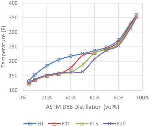
In some cases, MB targets seek to restore (raise) the value of T50 that might otherwise be suppressed by ethanol addition, requiring the addition of heavier components, but market ethanol blends have lowered T50. For comparisons of E15 or E20 with E10, nonlinear ethanol blending impacts are less profound than for the E0 to E10 step.

Most studies have been fuel-oriented, and have represented the vehicles by model year or by broad engine technology classification. However, it is clear that engine design and controls have strong effects on resulting emissions (Maricq, Szente, and Jahr 2012; Schulz et al. 2011).

CRC E-67

The 2006 E-67 study (Durbin et al. 2006) employed PFI automobiles and light trucks (2001–2003 California-certified LEV to SULEV) atypical of current model year technology, but still present in the national fleet. The study sought to control and quantify the emissions effects of T50 (3 levels), and T90 (3 levels) and ethanol volume (0%, 5.7%, and 10%), using a 12 fuel matrix. Aromatic volume, olefin, and saturate fractions each were held at approximately the same values in the gasoline fraction (BOB), without the market fuel tradeoff between ethanol and aromatic content that is driven by refinery economics. However, the molecular weights of the aromatics, olefins, and saturates would have varied between fuels to yield the targeted T50 and T90 properties. The antiknock properties of the fuels varied. E-67 yielded an emissions model, but the model does not predict the tradeoff of reducing aromatics when adding ethanol.

EPAct

The Energy Policy Act (EPAct) study (EPA 2013a, 2013b) examined 27 fuels in 15 PFI vehicles, all of the 2008 model year and meeting Tier 2 emissions standards. Study results have been used in emissions predictions within the EPA MOVES model (EPA 2018) that is used to evaluate emissions scenarios for a wide variety of applications. The program focused on the effects of ethanol (4 levels), aromatics (2 levels), RVP (2 levels), T50 (5 levels), and T90 (3 levels). The test plan used a reduced matrix of fuel parameter combinations. Fuels were MB using refinery blendstocks. Although properties were chosen to match market fuels, aromatics were included at only two levels, set at 15% and 35%, bracketing average typical commercial gasoline properties. Variables not selected for the study, such as distillation parameters other than T50 and T90, and anti-knock properties, were not controlled.

The study used the LA92 driving cycle to produce phase-level emissions of CO₂, CO, THC, methane (CH₄), non-methane hydrocarbons (NMHC), NOx, PM by mass and NMOG. The subsequent analysis led to the exclusion of data for certain vehicles. An EPAct Phase 3 report presented full and reduced statistical models to describe emissions in terms of fuel parameters. Models were developed in log space for each pollutant by phase. PM and NOx models were fitted to the data, and are employed below.

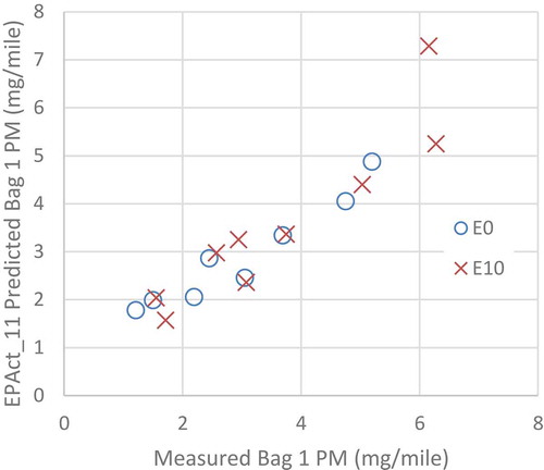
Figure 3 shows EPAct LA 92 Phase 1 (cold start) PM emissions data for the E0 and E10 fuels in the program, along with the emissions predicted by the EPAct 11 term model. Each of these points represents an average value for a fuel used in the 15 vehicles in the program: vehicle-to-vehicle variations are substantial and not shown in Figure 3.

Figure 3. Measured and modeled emissions of the E0 and E10 fuels in the EPAct study for LA92 Phase 1 PM

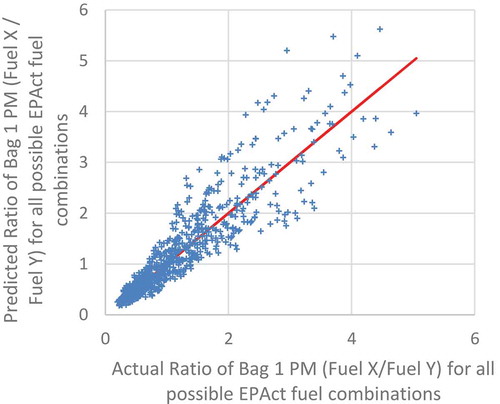
Figure 4 shows the ratios of LA92 Phase 1 PM emissions, averaged for all vehicles, as ratios between PM emissions using each of the 27 study fuels compared to all other 26 fuels. Although the EPAct models fit the overall data, Figure 4 shows that the predicted ratios of emissions for any pair of fuels can deviate substantially from the measured values for the same pair. Some of this may be ascribed to difficulty in measuring low emissions levels accurately, as well as the influence of precise composition outside of the major parameters. Models, therefore, cannot be expected to provide an accurate prediction for all fuel pairs.

Figure 4. Comparison of measured and predicted LA92 Phase 1 ratios of emissions of all of the 27 EPAct fuels with one another

Following the EPAct study, the CRC E-98/A-80 study (Jimenez and Buckingham 2014) used three additional fuels with the EPAct fleet. One fuel was a re-blend of an EPAct fuel, while the other two were an E10 with 27.4% aromatics and an E15 with 24.6% aromatics, lying between the EPAct 15% and 35% target aromatic levels. The EPAct study data were analyzed separately by Gunst (2013), who produced a baseline 17 term emissions model and reduced term models. The Gunst (2013) 11 term model, derived from the original EPAct data, predicted different emissions ratios between fuels than were measured by Jimenez and Buckingham (2014).

CRC E-94

CRC E-94-2 (MB) (Morgan et al. 2017) was the major phase of this study, which departed from prior studies by addressing only GDI technology. E-94-2 employed twelve 2011–2014 MY vehicles, both naturally aspirated and turbocharged. Eight fuels were used, with high and low values of AKI (87 and 93 AKI targets), PMI (1.4 maximum and 2.4 minimum targets), and ethanol (0% and 10%).

The LA92 drive cycle was used, with all three phases and a cold-start phase 1. Each vehicle and fuel combination had two runs, unless THC differed by 30% or more between the runs, or NOx or CO exceeded 50%. The study aimed to address several questions, including whether variables other than AKI, PMI and ethanol content affected emissions, and whether different engine technologies affected conclusions. Reid vapor pressure (RVP) was 6.5–7 psi for all of the fuels. Although T50 was held constant for the match blends, T40 varied. AKI was at 87 or 93, which would constrain blending due to the fixed aromatic levels. The investigators stated that the E-94-2 fuels met specifications and could be sold as commercial fuels, although this does not imply that they represent expected market blends.

Results from E-94-2 show that PM increased from 26% to 221% when PMI was raised from the low value to the high value, with ethanol and AKI held constant. AKI had mixed effects on PM, while ethanol (E10 vs. E0) reduced PM for one vehicle, and increased PM between 18% and 44% for the remainder. The statistical analysis and model for the study projected no CO, THC, or NOx effects for ethanol level. For the E-94-2 blends, although PMI was set to high and low levels, the PMI in each case was achieved with similar aromatic content for E0 and E10, emphasizing the difference between aromatic content and PMI as study parameters.

The E-94-3 (SB) component of the study (Morgan et al. 2018) diluted four E0 fuels from the E-94-2 program with 10% ethanol to produce four E10 SB fuels, with low and high AKI (91 and 96) and low and high PMI targets. Four GDI vehicles, two naturally aspirated and two turbocharged, were tested on a cold-start LA92 schedule. One of the four vehicles was noted to have anomalous emissions behavior. Overall, both PM mass and particle number rose with the addition of ethanol by splash blending, whether for three (excluding anomalous behavior vehicle) or four vehicles. The ethanol PM effect was far lower than the effect of PMI. The splash blending yielded lower PM mass than the E94-2 match-blended fuels, but statistical analysis suggested that this was not a defensible general conclusion.

CRC E-129

Recently CRC published results from the E-129 (SB) study, which examined tailpipe emissions of four 2012–2013 gasoline automobiles with 4-cylinder GDI engines over the LA92 cycle (Schuchmann and Crawford 2019). The project examined the effects of MTBE and isobutanol, as well as ethanol. An E0 low AKI, low-PMI fuel from the E-94-3 project (Fuel C) was re-blended and then blended with the three oxygenates to produce three additional fuels with a 3.5% oxygen target (including E10), and three more with a 5.5% oxygen target (including E15).

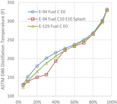
Figure 5 shows the distillation curves for E94-3 Fuel C, E-94-3 Fuel C splash blended to E10, and re-blended E-129 Fuel C. Figure 5 shows differences of 14.6 and 13.4 degrees F in the 20% and 30% distillation values between the E-94-3 original fuel and E-129 re-blend. The E-129 fuel C had a PMI of 1.26, in contrast to the value of 1.38 for the Fuel C of E-94-3, while most other parameters matched well between the two fuels. Aromatics for the SB E10 and E15 fuels in E-129 were reduced only by dilution with the oxygenates.

Figure 5. Distillation curves for E-94 fuel C (E0), re-blended E-129 fuel C (E0), and E-94 fuel C splash blended to E10. E-94

E-129 Results showed that E10 caused an insignificant change to PM (relative to E0), while E15 reduced PM significantly. Although NOx was lower on average for E10 and E15, there was no statistically significant difference from the E0 level. The CRC E-129 data for the E-15 were in contrast to the E-94-3 E-10 results, where PM increased with ethanol content. However, the vehicle test fleet was not the same between the two studies.

UCR Yang et al

A team from the University of California, Riverside, measured emissions from five 2016 and 2017 GDI vehicles on eight fuels (Yang et al. 2019a, 2019b). E0, E10, and E15 fuels were blended to target aromatic levels of approximately 20% and 30%. The E10 fuel with 20% aromatic content was a Tier 3 certification fuel. In this way, the targets for ethanol and aromatics were structured in a similar fashion to the EPAct study, but the aromatic content had a lower spread of values. Two additional fuels in the study were prepared by splash blending ethanol to E15 and E20 levels. The splash-blended E15 and the target-blended E15 had very similar properties. Octane ratings were 87 or 88 for the target blends and slightly elevated for the two splash blends. The T50 values of six fuels were naturally lowered by the ethanol addition. Emissions were measured using the LA92, by phase. Data showed a strong effect of aromatic content on the PM emissions for both the cold-start phase 1 and overall LA92 results.

Critique and differences between studies

The authors previously reviewed the first three studies presented above, along with numerous smaller studies (Durbin et al. 2006; Morgan et al. 2017; Whitney 2014), in a recent report (Clark et al. 2019a) and paper (Clark et al. 2019b) and found no unifying emissions effect conclusions. Variation in vehicle technology, test cycles, study structure, and fuel blending approaches contributed to the substantial difference between study results. In addition, emissions levels for modern vehicles are low, leading to high measurement variability.

Ethanol content, aromatic content, T50, T90, AKI, and PMI have all been examined for their effect on emissions. Other properties varied and were not necessarily considered as study variables, but may still have impacted the statistical analysis that was employed. Multivariate studies require a substantial count of fuels and test runs to have statistical significance and manage confounding parameters and are naturally resource-limited.

Although the E-94-2 fuel blending targeted four E0 and four E10, at two different PMI levels, all had the target of 25% aromatic content. This orthogonal study matrix did not reflect a tradeoff between ethanol and aromatics, and the blend properties of ethanol with a market BOB. Ethanol effects are sensitive to the BOB composition, and the ethanol content would generally imply a lowered aromatic content of a commercial BOB. PMI and aromatic content were not correlated: aromatics had different compositions between blends. The high PMI fuels corresponded with T90 values of 340 to 345 degrees F, compared to the low-PMI fuels with T90 of 305 to 311 Degrees F. The study fuel analyses show that the C10+ aromatics rose by a factor of almost three for the high PMI fuels with high T90.

In contrast to the use of PMI in the E-94-2 study, the EPAct study used aromatic content as a blending and modeling variable, along with RVP, T50, and T90. The relationship between market gasoline PMI and total aromatics is of interest, but no substantial comparative database is available for comparison.

Figure 6 shows the aromatic and ethanol content of the EPAct and E-94 fuels.

Figure 6. Relationships between aromatic and ethanol content for the EPAct and E-94 studies

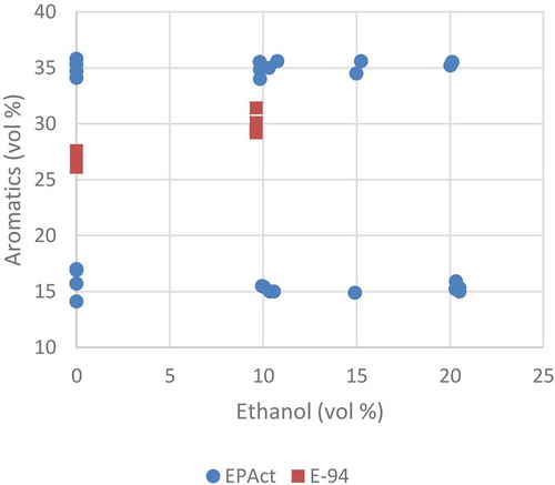
E94-2 fuels show a PMI spread (Figure 7), whereas aromatic content varied little (Figure 6). The E10 E-94 fuels have slightly higher aromatic content than the E0 fuels, and marginally higher PMI (Figure 7). The EPAact study separated ethanol and aromatic content through study design.

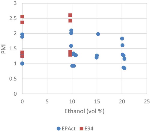
Figure 7. Relationships between PMI and ethanol content for the EPAct and E-94 studies

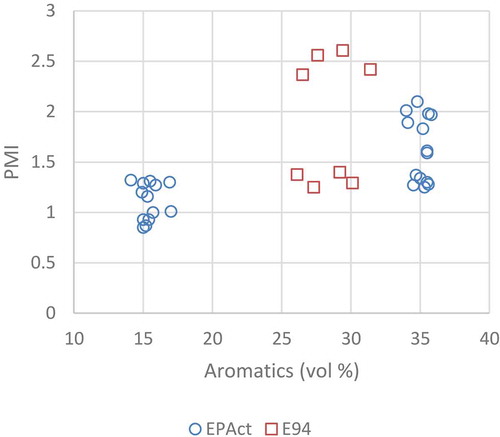
Figure 8 suggests that neither aromatic content nor PMI serves as a complete descriptor for a study, and shows differences in the PMI to the aromatic relationship between the EPAct and E-94-2 fuels suites. For the EPAct study, PMI loosely tracks aromatic content, while for E94-2 PMI was split and does not relate closely to aromatic content. About half of the fuels in the EPAct program have similar PMI but two widely spaced values of aromatic content, suggesting that the nature of the aromatic species varied substantially, while E-94-3 had two widely spaced values of PMI with a modest range of aromatic levels for both values. These two different sets of fuels were employed with two different engine technologies. EPAct addressed PFI vehicles while E-94 addressed GDI vehicles.

Figure 8. Relationship between PMI and aromatic content for the EPAct and E-94 studies

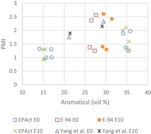
Figure 9 presents the variation of PMI with ethanol in the study fuels and includes the fuels recently used by Yang et al. (2019a, 2019b). In E-94 aromatics were higher in E10 that E0 fuels to meet E-94 PMI targets. The fuels of Yang et al. (2019a, 2019b) had levels of aromatics and PMI within the bounds of the EPAct and E-94-2 studies.

Figure 9. PMI and aromatic content separated by ethanol fraction for EPAct and E-94 fuels, and the fuels used by Yang et al. (2019a, 2019b)

Market fuels

Gasoline production and blending behavior

Gasoline sold in the US differs in composition between summer and winter and in octane rating. In the US, ASTM D4814-19 standards must be met for classes of gasoline: standards include distillation parameters, the driveability index (Jewitt, Gibbs, and Evans 2005) and RVP requirements. There are regional differences in gasoline composition, and the use of conventional gasoline versus reformulated gasoline (RFG) for air quality control (Bishop, Hoekman, and Broch 2017; Hoekman, Leland, and Bishop 2018). When ethanol is a constituent of the final product, refinery streams are blended to produce a BOB, and the ethanol and BOB are blended at a terminal. The blend must meet specifications, and the BOB is configured to support this obligation. Figure 10 shows the changing balance of U.S. refinery production since 2004.

Figure 10. In a decade US refinery gasoline production changed from predominantly finished product to predominantly BOB

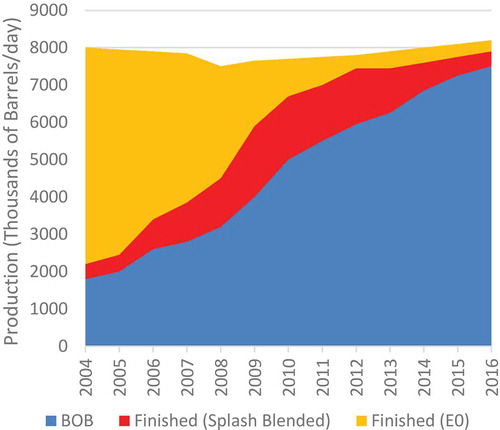
The refiner utilizes streams to blend the BOB that is most attractive for the overall economic benefit of the refinery, which produces additional products such as diesel, jet fuel, fuel oil, heating oil, petrochemical feeds, solvents, and liquefied petroleum gas, each with varying market value.

Typically, the AKI of the finished blend will not substantially exceed the pump decal value (Clark et al. 2019b) because raising octane adds production cost. Although both the crude feed and the refinery configuration will impact the precise composition of the BOB, it is blended from a number of streams available from distillation and process units. These streams include fluid catalytic cracker (FCC) output, reformate, alkylate, isomerate, and other sources such as light straight-run naphtha. Viewed in another way, these streams provide differing ratios of the major hydrocarbon groups, namely aromatics, olefins, and saturates (paraffins and isoparaffins). The streams also have differing spectra of molecular weights, which influence their volatility and distillation profiles. For additional detail see Clark et al. (2019a).

Relating fuel antiknock properties to major hydrocarbon groups is complex. Generally, aromatics are assumed to raise octane numbers and saturates are assumed to lower the number. However, straight-chain n-paraffins have substantially lower antiknock properties than branched-chain iso-paraffins, as evidenced by alkylate properties. Even within the iso-paraffin realm, there is substantial variability in performance: methyl hexane as a pure C7 iso-paraffin has a Research Octane Number (RON) of under 50, whereas trimethyl butane (another C7 iso-paraffin) exceeds 110 (Ghosh, Hickey, and Jaffe 2006). For aromatics, n-propyl benzene has a RON of 102, but trimethyl benzene has a RON of more than 120. Adding complexity, there is a functional interaction between different hydrocarbons in a fuel. A hydrocarbon mixture may exhibit a RON that is higher than, or lower than, the linear combination of its components. Researchers have addressed the complexity of predicting the anti-knock properties of blends (Foong et al. 2014; Anderson et al. 2012). These interactions lead to the concept of a blending octane number, based on the differential change in octane number when a specific compound is added to a mix of other hydrocarbons. The composition of a BOB will, therefore, affect the blending octane number.

The effect of ethanol between 0% (E0) and 10% (E10) differs substantially from the effect between E10 and E20: rate of change in major blend properties is far from linear. Refineries lower the octane of the BOB, typically with reduced aromatic content, to take advantage of the high-octane blend characteristics of ethanol. This allows aromatics to be sold in other markets or else reduces the burden on the refinery reformer, which produces aromatics.

Where fuels are tailor-made to match selected target parameters, other fuel parameters and properties may vary in an unexpected fashion. In preparing test fuels by blending to match a limited parameter count, variabilities of detailed hydrocarbon properties constrain the applicability of the results to unseen fuels. As an example, blends with the same distillation properties and aromatic content may differ substantially in the propensity to limit knock or produce particulate matter, because the aromatics may be concentrated in different parts of the distillation curve, and the saturates may vary in their branched structures.

Market fuel composition

The 2006–2016 historic trends in Figure 1 show an aromatic reduction of 0.81% for a 1% addition of ethanol, but market forces, MTBE removal, and olefin and benzene reduction were also at play over the last two decades. E10 is now the national norm, but a present-day scenario for E0 should not be predicated quantitatively on a reversal of the Figure 1 history. Table 1 presents representative summer regular blend E10 properties based on available Automobile Alliance and EPA fuel quality trends data.

Table 1. Representative summer regular AKI blend properties based on available automobile alliance fuel data and EPA fuel quality trends

	E0	E10	E15
API	57.1	58.7	57.4
Vap. Press, psi (EPA)	8.2	8.2	7
Distillation, Deg. F
10% evap.	136	129	129
20% evap.	161	138	138
30% evap.	191	146	148
40% evap.	207	156	156
50% evap.	219	192	162
60% evap.	234	224	208
70% evap.	251	249	247
80% evap.	283	279	279
90% evap.	325	320	320
Aromatics, V%	32	21.8	17.4
Olefins, V%	9	8.1	7.65
Saturate, V%	59	60.1	59.9
RON	92.1	92.2	92.4
MON	83.4	83.3	83.1
AKI	87.8	87.8	87.8

E0 and E15 quality parameters were calculated from the E10 properties based on parameter blending correlations, as presented previously by Clark et al. (2019a). The blending parameter change assumes an economical approach for creating a substantial present-day E0 supply, namely blending of more reformate or increase of reformer severity. Without oxygenate use, the aromatic percentage would rise at about the same percentage that ethanol is lost to maintain octane rating, in support of Table 1. Tamm et al. (2018) attest to the availability of reformer capacity to pursue this pathway, with 2016 reformer utilization below 80%.

Table 1 also includes parameters for E15, adjusting the aromatics downward from the E10 value by 4.4% for the 5% ethanol addition. The positive effect, or boost, of ethanol on AKI depends on the composition of the BOB, but the change of AKI with respect to ethanol fraction is fairly constant from E0 to E15 (API 2010), suggesting that the aromatic reduction should remain linear. Most present-day E15 is splash blended using an E10 BOB, resulting in an elevated AKI of 88, with aromatics reduced only by dilution. The Table 1 parameters assume a dedicated E15 BOB that holds the summer regular AKI at 87. Essentially, the compositions in Table 1 hold the saturate and olefin levels to be similar for E0, E15, and E10, so that the sum of ethanol and aromatic volume fraction also remains fairly constant. Increased use of alkylate rather than reformate to raise octane rating would lower aromatics and raise saturates for any of the fuels in Table 1. Properties of regular summer E10, E15, and E0 values, as shown in Table 1, have been used as model inputs below.

Modeling and comparison

Several emissions models derived from EPAct study data for 2008 PFI model year vehicles have been employed below to compare the ethanol effect measured by other studies and to predict the ethanol effect from expected in-use blends. The intent was to examine the general applicability of models and the extent to which they could address unseen data.

The EPAct data yielded two models, based on 11 candidate terms and 17 candidate terms. The models use ethanol and aromatic content, T50 and T90, and higher order effects to predict PM and NOx emissions. These models are best used in a comparative sense to predict the ratio of emissions between two fuels. However, these models are also capable of direct prediction of emissions relative to average emissions values in the EPAct study. Additional statistical terms must be added to the fuel property terms for absolute emissions prediction.

Gunst used the EPAct data to produce a reduced model, used below, and Butler et al., in revisiting the EPAct data, used PMI as a study variable to predict PM, with good success in fitting the EPAct study data (Butler et al. 2015; Gunst 2013).

Although PMI, also used in the E-94 studies, is influenced strongly by the presence of aromatics with a high boiling point, it cannot be mimicked reliably by the use of aromatic content, T50 and T90 because some aromatics (such as toluene) are light, whereas high boiling point species may include straight-chain saturates. Figure 7, discussed above, shows the PMI and aromatic content for both the E-94-2 and EPAct studies, and suggests that these two variables are not unequivocally correlated. If PMI and aromatic content correlate with measured emissions in different ways, it is likely that the weighting ascribed to other variables (such as distillation parameters and ethanol content) will differ.

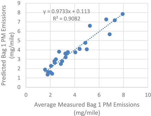
A critique of the EPAct analysis advocated for use of T70 as a statistical variable and showed that E15 reduced PM emissions by a substantially greater percentage when T70 was employed (Darlington et al. 2016). Several models were offered, as fits to the EPAct data. Darlington et al. found that they could fit the data with a slightly greater measure of success using only the aromatic content and values of T70 and (T70)². In this way, Darlington et al. replaced T50, T90, and ethanol in the predictive model by using T70. Figures 11-Figure 15 show the fits of five models (Table 2) to the EPAct data for the 27 fuels, averaged across the vehicle fleet.

Table 2. Coefficients for five PM models based on the EPAct data

	EPAct11 Term	EPAct17 Term	Butler PMI	Darlington T70	Gunst Reduced
Intercept	0.6559	0.6529	0.6559	0.627	0.6540
Aromatics	0.3833	0.3792		0.265	0.4202
T90	0.2923				0.3356
EtOH	0.1582	0.3034	0.2287		0.1722
T50 x T50	0.0935	0.0806			0.1247
T50	0.0550	0.1004	0.1063		0.0285
EtOH x T90		0.0647			0.0611
Aromatics x T90		0.0665
PMI			0.4815
PMI x EtOH			0.0836
T70				0.3658
T70 x T70				0.1138
RVP					−0.0316
EtOH x Arom					0.093
RVP x T90					−0.0708
T90 x T90					0.1011
Εσ2	1.0359	1.0359

Figure 11. Fit of the 11 term EPAct model with the EPAct measurements

Figure 12. Fit of the 17 term EPAct model with the EPAct measurements

Figure 13. Fit of the Butler et al. PMI model with the EPAct measurements

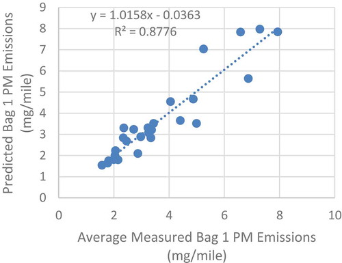
Figure 14. Fit of the Darlington et al. model with the EPAct measurements

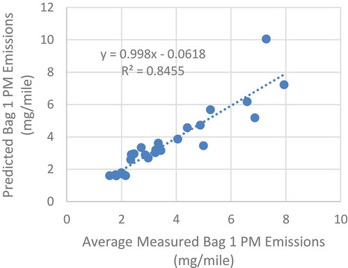
Figure 15. Fit of the Gunst reduced model with the EPAct measurements

It is of interest to see how the models extend to fuels with unseen properties and to the comparison of emissions from two fuels in more recent technology vehicles.

Predictions of market gasoline blend effects

This section describes the use of both EPAct-measured data and EPAct-derived models for determining relative emissions effects between the summer regular E0 and E10 fuels with compositions shown in Table 1, and termed SR0 and SR10. No single EPAct fuel closely matched either SR0 or SR10, in part because the EPAct values for aromatics bracketed both SR0 and SR10 aromatic levels. However, apportioned mixtures of two EPAct fuels proved able to approximate SR0 and SR10. Two pairs of EPAct fuels were selected to achieve similar T50 and T90 distillation temperatures as SR0 and SR10. The two fuels in a pair were then weighted based on the volume percentages aromatics of the representative summer E0 and E10 fuels. There were assumptions of linearity used in this selection and weighting, but the process does allow for some direct empirical data comparison before examining global model predictions.

A weighted average of EPAct fuels 6 and 11 best approximated the T50 and T90 distillation temperatures of the summer E10. The apportioning volume percentages required to achieve the SR10 aromatics content (21.8%) were 65% of EPAct Fuel 6 and 35% of EPAct Fuel 11. Using the same methodology for SR0 resulted in an apportioned mixture of EPAct fuels 8 (11%) and 13 (89%). The matching process is summarized in Table 3.

Table 3. SR0 and SR10 fuels were matched as closely as possible using two combinations of two study fuels used in the EPAct study

	Summer E10	EPAct Fuel 6	EPAct Fuel 11	65% EPAct Fuel 6 + 35% EPAct Fuel 11	Summer E0	EPAct Fuel 8	EPAct Fuel 13	11% EPAct Fuel 8 + 89% EPAct Fuel 13
Ethanol	10%	10.6%	10.3%	10.5%	0%	0%	0%	0%
Aromatics	21.8%	15%	35%	21.8%	32%	15.7%	34.1%	32%
T50 (^oF)	192	189	189	189	219	221	222	222
T90 (^oF)	320	340	299	326	325	303	338	334

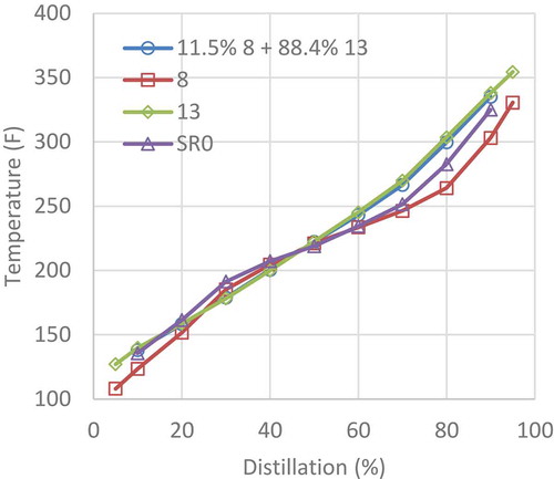
Assuming linear blending properties, the distillation characteristics were determined from the percentages of the two fuels, vaporized as a function of temperature, then combined and inverted. Figures 16 and Figure 17 present the distillation curves gained using this method. In both cases, the EPAct mixes have a slightly higher T90 than the market fuels of Table 1. Differences were largest around T80, being 14 degrees for SR10 and 17 degrees for SR0. However, the differences are in the same direction, so that ratios of emissions using SR10 and SR0 should be less affected.

Figure 16. The distillation curve for the SR10 is compared with the computed curve for a mix of EPAct fuels 6 and 11

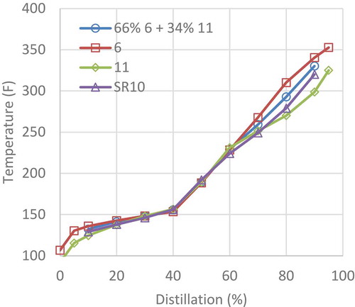
Figure 17. The distillation curve for SR0 compared with the computed curve for a mix of EPAct fuels 8 and 13

This apportioning exercise, using the same percentage values, was extended to include measured and predicted SR0 and SR10 emissions from the EPAct study data and models. The Phase 1 data from the LA92 were used exclusively because the cold start represents a high emissions inventory contribution.

The average-measured LA 92 Phase 1 PM emissions from vehicles in the EPAct study for fuels 6 and 11 were 2.98 and 3.25 mg/mile, respectively. These values were calculated as bulk-averaged emissions excluding data from one vehicle in the study (Ford Focus), which was also excluded from EPAct modeling. Bag 1 PM measured emissions using the fuel mix percentages (65% EPAct Fuel 6, 35% EPAct Fuel 11) yielded estimated emissions of 3.07 mg/mile, as shown in Table 4. The EPAct 11 term model for phase 1 PM predicted emissions of 2.57 and 2.94 mg/mile from fuels 6 and 11, so that SR10 emissions would be 2.70 mg/mile if the modeled values were proportioned. Bag 1 PM emissions predicted using the EPAct 11 term model directly from the summer E10 fuel properties, were 2.45 mg/mile.

Table 4. Emissions of LA 92 phase 1 PM from SR0 and SR10 estimated from proportioned emissions from actual EPAct vehicle data (in mg/mile)

	Measured	Predicted
EPAct Fuel 6	2.98	2.57
EPAct Fuel 11	3.25	2.94
Apportioned Emissions 6&11	3.07	2.7
Apportioned Properties 6&11		2.69
SR10		2.45
EPAct Fuel 8	1.99	1.5
EPAct Fuel 13	4.88	5.2
Apportioned Emissions 8&13	4.56	4.79
Apportioned Properties 8&13		4.51
SR0		3.8

Table 4 shows that the absolute measured and predicted EPAct emissions differ, which is to be expected noting that the models were derived from a large database. Table 4 also shows good agreement between the averages of single fuel prediction and the predictions of the two pairs with apportioned properties. The two pairs differ by a ratio of 1.49 using the measured values, compared to 1.41 for the EPAct model predictions for SR0 and SR10.

Table 4 values build confidence in the approach, although it is approximate, and suggest that the PM emissions for SR10 were 67% (pair measurements), 60% (apportioned properties), or 56% (apportioned properties) of the SR0 emissions. This reduction for SR10 over SR0 is not attributed directly to the ethanol in the fuel, but to the reduced aromatics and T50 values that accompany the blending relative to an E0 market fuel with the composition shown in Table 1, assuming the use of reformate versus ethanol to maintain AKI.

The analysis was extended to include the EPAct 17 term model, the Butler et al. model and the Darlington model as well. Table 5 presents the results. Since PMI values were not available for the SR0, SR10, and SR15 fuels, these cells are not filled for the Butler model. In all cases, whether by direct prediction, or by a prediction for the best-fit EPAct fuel mixes, SR0 emissions are substantially higher than SR10 and SR15 emissions. The two EPAct models predict similar emissions for SR10 and SR15 compositions shown in Table 1. Gunst shows slightly higher PM emissions for SR15 than SR10. The Darlington et al. model, which predicts the EPact study fuel emissions equally well but has a substantially different formulation, differs from EPAct in its prediction of SR0, SR10, and SR15, and shows an emissions reduction for SR15 over SR10. This is, in part, due to the use of T50 and T90 in matching fuels, whereas Darlington uses T70 for computations. Nevertheless, the model of Darlington et al. shows that SR15 has PM emissions that are 64% of SR0, in strong agreement with the 64% and 62% values for the two EPAct models. A conclusion is that all models show a substantial increase in SR0 PM emissions over SR10 and SR15 emissions for an even volumetric percentage tradeoff of ethanol and aromatics in the blends. Prior research by the present authors using the EPAct 11 term model showed that the PM increase for E0 was present without such substantial aromatic addition due to the increase in T50 for E0: this increases PM in the EPAct 11 term model (Clark et al. 2019a).

Table 5. Five models were employed to predict PM emissions from phase 1 of the LA92 in pursuit of determining the emissions difference between SR10 and SR0. Prediction for SR15 is also shown

	Measured	EPAct11	EPAct16	Butler PMI	Darlington T70	Gunst
EPAct Fuel 6	2.976	2.573	2.460	2.595	2.687	2.792
EPAct Fuel 11	3.251	2.942	2.726	2.756	3.190	3.215
6&11 Blend (Property)		2.693	2.715	2.649	2.788	2.045
6&11 Blend (Apportioned)	3.072	2.702	2.553	2.651	2.863	2.904
SR10		2.446	2.486		2.169	1.773
SR15		2.449	2.370		1.880	1.841
EPAct Fuel 8	1.993	1.501	1.734	1.494	1.781	1.625
EPAct Fuel 13	4.875	5.200	5.160	4.661	4.725	3.215
8&13 Blend (Property)		4.512	4.455	4.090	4.144	3.729
8&13 Blend (Apportioned)	4.543	4.774	4.766	4.297	4.386	3.033
SR0		3.797	3.803		2.949	2.663

Similarly, LA92 Phase 1 NOx emissions were also projected for SR0, SR10, and SR15, as shown in Tables 6 and Table 7. Neither Butler et al. nor Darlington et al. offered alternate NOx models.

Table 6. Phase 1 NOx emissions as measured and predicted using the EPAct models

	Measured	EPAct11	EPAct17
EPAct Fuel 6	0.0731	0.0515	0.0561
EPAct Fuel 11	0.0536	0.0699	0.0690
6&11 Blend (Property)		0.0564	0.0589
6&11 Blend (Apportioned)	0.0662	0.0579	0.0606
SR10		0.0564	0.0583
SR15		0.0534	0.0580
EPAct Fuel 8	0.0625	0.0486	0.0451
EPAct Fuel 13	0.0840	0.0660	0.0637
8&13 Blend (Property)		0.0637	0.0630
8&13 Blend (Apportioned)	0.0816	0.0640	0.0616
SR0		0.0634	0.0643

Table 7. Phase 1 E10/E0 NOx emissions ratios for apportioned EPAct fuel blends and representative summer regular AKI fuels

	Measured	EPAct 11	EPAct 16
E10 (6&11 Blend)/E0 (8&13 Blend) – Property		0.885	0.935
E10 (6&11 Blend)/E0 (8&13 Blend) – Apportioned	0.812	0.905	0.984
SR10/SR0 (Property)		0.900	0.907
SR15/SR0 (Property)		0.842	0.902

SR15 showed NOx reductions of 16% and 10%, while SR10 showed NOx reductions of 11% and 8% relative to SR0. Measurements of the comparable mixes (the same apportionment as for PM analysis) suggested a 19% reduction for SR10.

Whether by measurement of comparable mixes or modeling of comparable mixes or modeling of the Table 1 fuels themselves, modest reductions in LA92 Phase 1 NOx are found for the blending of ethanol based at the 10% to 15% level, and displacing aromatics based on the EPAct data. Reductions in PM were more substantial, as a percentage.

Predictions for GDI vehicles

There are strong arguments that PFI and GDI vehicles may react to fuel property changes in different ways. The PFI vehicles provide for substantial evaporation ahead of the intake valve, whereas the GDI vehicles inject directly into the cylinder, where homogeneity can be difficult to establish for late injection. Further, GDI spray and timing strategies vary and are still evolving (Martinez, Merola, and Irimescu 2019; Short et al. 2017). A confounding measurement factor may also be the ability of ethanol to dissolve existing engine deposits, which Sakai and Rothamer observe “is worth keeping in mind when considering data from studies comparing ethanol-gasoline blends at varying blend levels.” (Sakai and Rothamer 2019).

Comparison of measured emissions (mg/mile values) in the EPAct study for PFI vehicles and the E94-2 study for GDI vehicles immediately reveals that the PM emissions levels from the two technologies differ, so that data from one study should not be used to predict absolute emissions from the other study quantitatively. However, it is of interest to see how accurately the EPAct-based (PFI, MB) models might predict the emissions ratios between the two fuels used in E94-2 (GDI, MB). The properties for the eight study fuels in E94-2 were AKI (high and low), PMI (high and low) and ethanol (E0 and E10). E94-2 presented modeled emissions in the report, with measured emissions also available. The E94-2 PM emissions were expressed as a ratio for four fuel pairs, each representing an E0 fuel and an E10 fuel with the same target AKI and PFI. These emissions ratios do not reflect the tradeoff between aromatics percent and ethanol percent as presented in Table 1 and discussed above, since aromatics were higher in the E10 study fuels than in the E0 study fuels. Coefficients for the EPAct 11 term model (see Table 2) would anticipate higher PM emissions when both ethanol and aromatics are raised simultaneously.

Figure 18 presents comparative E10 and E0 emissions from the GDI E94-2 data and E-94-2 fitted model, along with predictions from the models developed from the EPAct data. The disagreement was highest for the two ratios of fuel pairs B/D and F/H, which represent high PMI. The EPAct 11 term model showed the best agreement with the measured fuel ratios, but generally overestimated the ratios. For the Fuel F/H ratio, the high PMI and high AKI fuels elicited a strong contrast between the Butler et al. and Darlington et al. models, the latter being the closest prediction of all four models. Disagreement may be attributed to the disparate relationships between PMI and aromatics in the E94-2 and EPAct studies (as shown in Figure 7), or due to the differing distillation curves, or simply due to the behavioral differences between GDI and PFI vehicles in the studies.

Figure 18. Measured and predicted percentage differences between GDI E10 fuel emissions and GDI E0 fuel emissions. [A/C represents emissions increase on E10 fuel A relative to emissions on E0 fuel C]

Figure 18 suggests that a PFI-derived predicted ratio should not be employed as an emissions adjustment factor when considering GDI vehicles in the fleet, and presumably vice versa. Further, the model execution shows that whereas the EPAct-derived models all fitted the EPAct data reasonably (see Figures 11,Figures 12,Figures 13,Figures 14-Figure 15), they diverged in predicting emissions ratios of the E-94 unseen fuels.

Match versus splash blending

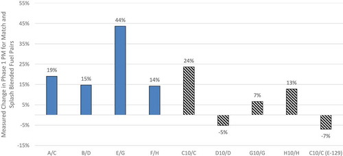
MB (where parameters other than ethanol content had target values), SB (where the ethanol diluted other components) and an approach where aromatics were reduced as ethanol was added are each likely to present different relative emissions data. Figure 19 compares LA92 Phase 1 PM-measured emissions of low-AKI, low-PMI E10 and E0 fuels from E-94-2 (Fuels A and C, Match), E-94-3 (E0 and E10 Fuel C, Splash) and E-129 (E0 and E10 reblended Fuel C, Splash). E-94-2 included data from 12 vehicles tested on both the E10 and E0 fuels, while E-94-3 included data from a four-vehicle subset of the original 12 vehicles. Additionally, E-94-3 considered a three-vehicle subset (one vehicle that exhibited inconsistent performance). E-129 used a different four-vehicle set, and a three-vehicle set is also shown (again, one vehicle with inconsistent performance excluded). All three studies developed predictive models based on their fuel matrices. The smaller sets of vehicles used in E-94-3 were matched to E-94-2 vehicles using emissions data included in both reports: this yielded the corresponding three and four vehicle averages for E-94-2.

Figure 19. Effect of 10% ethanol blending on Phase 1 PM emissions from CRC GDI studies (E-94-2, E-94-3, E-129). Number of vehicles in each average is in parentheses. E-94-2 three and four vehicle groups represent the same vehicle groups as for E-94-3. The E-129 vehicle group differs. The Yang et al. result compares a 29% aromatic E0 and a 21% aromatic E10

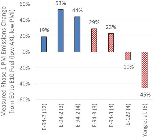
The E-94 PM increase for E10 relative to E0 reflects the use of the same aromatic content and PMI for E10 and E0 match blends, and only splash blend dilution for the splash blend case.

Differences between MB and SB contribute to variation in Figure 19, even when the same vehicle fleet was used. Figure 19 shows that SB E-94-3 LA92 Phase 1 emissions were higher than the MB values when all 12 E-94-2 vehicles were considered, but lower when compared to the same three of four vehicle sets in E-94-2. The E-129 study included a different subset of four vehicles from the E-94-3 study. Vehicle fleet influence may explain in part the contrast between the E-94-3 and E-129 data, where one study showed elevated PM emissions, while the other showed a reduction.

An additional E10/E0 comparison is also presented in Figure 19 for the five vehicle average from the Yang et al. Fuel 3 (E10, 21.4% aromatic, PMI 1.888) and Fuel 2 (E0, 29.4% aromatic, PMI 2.330), where those two fuels were chosen by the authors to illustrate effects of substantial reduction of aromatics along with ethanol blending (Yang et al. 2019a, 2019b). The aromatic content values are close to those of the Summer Regular E0 and E10 (SR0 and SR10) values in Table 1, and the PM reduction percentage is similar to data shown in Table 4 for SR0 and SR10. AKI is close for both fuels, but T90 is higher for fuel 2. This ratio in Figure 19 is in strong contrast to the match and splash blend effects, and emphasizes the importance of considering all parameter changes when comparing two fuels. GDI data from the same study, cold-start Phase 1 of the LA92, show that for both 20% and 30% aromatic gasoline E10 PM emissions were higher than E0 PM emissions when the aromatic level was held constant.

Fitted GDI data from E-94-2, E-94-3, and E-129 are compared with PFI model match and splash ratio predictions in Figure 20. All E-94 data are for Fuel C, and E-129 data are for reblended Fuel C. The SB PM differs in direction and scale, while the MB data differ only in scale, all presenting a PM emissions increase. Models are variable in their prediction of the match and splash-blended E10 PM change, but generally, the models show a lower ratio for the splash blends. Comparison of measured and predicted percentages differences suggests that PFI-based modeled ratios do not reflect GDI emissions ratios.

Figure 20. Comparison of emissions from E10 in comparison to E0, showing ratios of LA92 Phase 1 PM emissions for E-94-2 (MB, with 12 vehicles), E-94-3 (SB, with 3 and 4 vehicles), and E-129 (SB 4 vehicles). Both MB and SB emissions predicted emissions ratios are also presented for five models of the EPAct data

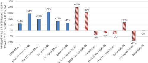
Fitted overall percent changes associated with CRC GDI studies for the E0 to E10 step are shown in Figure 21. The four MB ratios do not reflect the reduction of aromatics that would be anticipated in market fuel blending, since the aromatic content rose slightly with ethanol. The four splash-blended E-94-3 increases in PM are lower on average than their match-blended counterparts, but arose from a smaller set of vehicles. The E-129 study, with a different vehicle set from E-94-3, showed a splash blend reduction in PM of 7%, as opposed to the E-94-3 splash blend increase of 24% for a very similar composition of low AKI, low-PMI fuel (Fuel C) emissions (Yang et al. 2019b).

Figure 21. The E-94-2 fuels were paired to have similar AKI and PMI properties, and the ratio of the E10 fuel PM emissions to the E0 fuel PM emissions was compared for Phase 1 of the LA92. The splash blends were also included

E15 emissions

Fewer data exist in major studies to describe the effect of E15 and mid-level blends of ethanol than for studies of E0 versus E10. E-94-2 (match blended) and E-94-3 (splash blended) GDI studies addressed only E10. Vertin et al. reported a study where 12 2009 MY PFI vehicles of four types and six 2000 MY PFI vehicles of two types were aged on E0, E15, and E20 road fuels and emissions tested at intervals on E0, E15, and E20 splash-blended certification fuel and ethanol (Vertin, Glinsky, and Reek 2012). PM data were not reported, NOx emissions were not statistically different for the ethanol blend fuels, while NMHC and CO either remained the same or were lowered. Knoll et al. reported a 16 PFI vehicle study with model years ranging from 1999 to 2007 (Knoll et al. 2007). They used the LA-92 cycle and splash blends of certification fuel with up to 20% ethanol (E0, E10, E15, and E20). Overall NMHC were reduced as ethanol content increased. NOx and NMOG showed no statistical change.

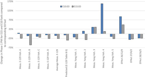
The effect of E15 on LA92 Phase 1 PM was examined for the recent E-129 data on four GDI vehicles, and for the EPAct program, using a PFI fleet. Whereas E-129 used 0%, 10%, and 15% SB of the same gasoline, for examining EPAct results, three “triplet” sets of three target fuels, representing E0, E10, and E15 were chosen, as shown in Table 8. One triplet has high aromatics and low T50 values, one has low aromatics and high T50 values, and one has high aromatics and high T50 values. The EPAct fuel T50 values are lower for the E10 and E15 blend than the E0 blends. Other properties (including RVP) do not match precisely. The blends do not reflect the tradeoff of aromatics and PMI with ethanol that is seen in commercial gasoline, but they offer modeling insight into the ethanol effect without adjustment for aromatic content or PMI. PMI is substantially constant within each data triplet in Table 8.

Table 8. Three groups of EPAct fuels, each with an E0, an E10, and an E15 fuel, selected to match other properties as closely as possible to determine the ethanol effect

EPAct Fuel ID	EtOH	Arom	RVP	T50	T70	T90	PMI
26	15.2	35.6	10.2	160	277	339	1.98
12	9.8	34.8	10.1	152	275	340	2.10
9	0	35.8	10.3	193	260	342	1.97
27	14.9	14.9	7.0	222	275	340	1.20
4	9.9	15.5	10.0	222	270	338	1.31
2	0	14.1	10.2	237	272	340	1.32
28	15.0	34.5	6.9	217	252	299	1.27
16	10.8	35.6	7.1	219	252	301	1.28
5	0	34.7	7.0	237	258	300	1.37

Figure 22 shows the resulting individual vehicle comparisons of the Phase 1 LA92 PM ratios for the E10/E0 and E15/E0 ratios from E-129. With one exception, all four of the E-129 vehicles show reductions of PM for E10 the data averages for E-129, and the E-129 predicted value. For E15 the reductions are unanimous and far greater than for E10. One of the three EPAct fuel triplets shows a substantial increase in PM for both E10 and E15, but the other two triplets show reductions for both E10 and E15, with E15 having similar reduction to E10. Figure 22 also shows UCR data for 20% aromatic E0, E10, and E15 fuel for five GDI vehicles (Yang et al. 2019b). Vehicle-to-vehicle PM emissions variations are noteworthy.

Figure 22. Comparison of E10/E0 and E15/E0 Phase 1 LA92 PM ratios for E-129, Yang et al., and selected EPAct fuel triplets (shown in Table 8)

The assertion that E15 produces lower PM emissions than E10 and E0 is well supported but not unanimous. Sabotowski et al. found that a GDI vehicle produced statistically lower PM on E15 than E0 on the 06 USD, but more PM on Phase 2 of the LA92 (Sobotowski et al. 2015). They also found varying results for three PFI vehicles. Another study showed no statistical difference for E0 and E10 PM mass emissions on the FTP cycle for two GDI automobiles but did show values for E20 PM that were lower (one statistically lower) than for E15 (Karavalakis et al. 2014). Oak Ridge National Laboratory examined a single 2007 GDI vehicle on the FTP and 06 USD (Storey et al. 2010). NOx emissions were lowered appreciably by ethanol addition (E10 and E20), with the E20 value at half of the E10 value. NMHC were lower for E10 but higher for E20. CO emissions varied little. On both the FTP and the 06 USD, the PM emissions were lowered by E10, and further lowered by E20 (Storey et al. 2010).

Averaged results from Yang et al. showed that for 20% aromatic content, cold-start LA92 PM emissions of E15 were similar to the E0 level, and below the E10 level. Splash blending the E10 to E15 reduced PM emissions, and further splash blending to E20 reduced PM further (Yang et al. 2019b). These blends of ethanol with 20% aromatics yielded Phase 1 PM LA92 emissions far below the E0 30% aromatic fuel, showing that aromatic reduction, enabled by ethanol increase, is a key to PM reduction. For the 30% aromatic level there was no statistically significant change associated with ethanol blending, although the measured values for E10 and E15 were slightly higher than for E0.

Conclusion

There are two different pathways for comparing real-world emissions due to a change in ethanol content. A comparative or pairwise study employs fuel compositions that would represent the candidate and baseline fuels marketplace. Alternately, a multivariate study examines several relevant fuel properties (including ethanol content) and employs statistical modeling to create a tool for emissions prediction of market fuel compositions. Either approach requires knowledge or estimation of relevant market fuel properties. Prior multivariate studies have been constructed in different ways, and applied to varying engine technologies, and so that there is no consensus on ethanol effects on atmospheric emissions. However, it is essential to consider all fuel parameter and composition changes when predicting differences in emissions effects from two market gasolines.

Five different models derived from the same PFI vehicle data set did not predict LA92 phase 1 PM emissions changes for unseen fuels closely, but all five showed substantial reductions of PM for E10 and E15 compositions with reduced aromatics relative to E0. The five PFI-based models also diverged when applied to predicting emissions ratios using an unseen set of fuel properties from the more recent E-94-2 GDI MB study. It is concluded that predictive models are limited in their ability to be extrapolated, both to unseen fuels and to vehicles of different technology.

The gross average MB data from E-94-2 for Phase 1 of the LA92 were compared with the SB data from the subsequent E-94-3 and E-129 studies. The SB data for three and four vehicle cohorts were higher than the MB data for a twelve vehicle cohort, leading to the conclusion that the vehicle test cohort needs to be large for reliable inventory prediction and that vehicle effects are a statistical concern.

E15 fuel PM emissions were also examined, as a ratio to E0 emissions, and compared to the E10/E0 emissions ratio. Both E-129 data (SB, GDI) and data from EPAct selected fuel triplets (MB, PFI) showed a wide variation between E10 and E15 effects in comparison to E0 emissions. It is difficult to draw unifying conclusions on both E10 and E15 effects, but generally, E15 presents lower phase 1 LA92 PM emissions than E10.

More conclusive data are required for emissions of ethanol blends in GDI vehicles, and data gained using market fuel composition tradeoff between ethanol content and aromatic content would be valuable. Further, very low emissions from late MY vehicles and the influence of individual vehicles in a study cohort challenge the ability to gain conclusive results for emissions ratios, particularly from small studies.

Acknowledgment

This study of emissions effects of ethanol blending was supported by the Urban Air Initiative.

Disclosure statement

No potential conflict of interest was reported by the authors.

Additional information

Funding

This work was supported by the Urban Air Initiative.

Notes on contributors

Nigel N. Clark

Nigel N. Clark holds a B.Sc. in Chemical Engineering and a Ph.D. in Engineering from the University of Natal in South Africa. His broad expertise is in energy systems research and development, with emphasis on engines, fuels, emissions, and transportation. He served on the faculty of West Virginia University (WVU) for 34 years, held the George Berry Chair of Engineering, and is a Emeritus Professor of Mechanical and Aerospace Engineering at WVU. Early in his academic career, Professor Clark was honored as a National Science Foundation Presidential Young Investigator by George H.W. Bush. He has conducted programs for the Departments of Energy, Defense and Transportation, the EPA, NASA, numerous state governments, federal government laboratories, the Environmental Defense Fund, the World Bank, the International Council for Clean Transportation, the Coordinating Research Council, major energy corporations and engine manufacturers. Dr. Clark is a Fellow of the Society of Automotive Engineers and has authored or co-authored 500 papers and technical presentations.

David L. McKain

David L. McKain holds an M.S. in Mechanical Engineering from West Virginia University. He currently directs and executes EPA certification testing of locomotives for Norfolk Southern and the American Association of Railroads. During his twenty-five year professional career he has directed and/or participated in numerous projects related to emissions and performance heavy-duty engines, vehicles, fuels and aftertreatment systems and has authored or co-authored numerous research articles. He has authored or co-authored over 50 peer-reviewed journal and technical papers. Mr. McKain has broad experience with fuel chemistry having conducted engine emissions and performance testing with both liquid and gaseous fuels including novel work with fuel blending and engine knock as well as comparative testing for federal and state regulatory certification. He currently works with the West Virginia University Research Corporation as a supervisory engineer.

Tammy Klein

Tammy Klein is the principal consultant for Future Fuel Strategies which provides market and policy analysis on transportation fuels for clients in the auto, oil and associated industries, as well as governments and NGOs. She was formerly Senior Vice President for Stratas Advisors/Hart Energy overseeing all aspects of its fuels and transport-related research, products, services, staff and consultancy. Tammy has served as an advisor to numerous companies, governments and NGOs on transportation fuels issues, including the Organization of Petroleum Exporting Countries (OPEC), International Petroleum Industry Environmental Conservation Association (IPIECA), Energy Management Authority (EMA) of Singapore and Natural Resources Defense Council (NRDC) and the, International Energy Agency (IEA). She holds a B.S. in journalism from the University of Florida and a J.D. from the Georgetown University Law Center with bar admissions in both the District of Columbia and Virginia.

Terence S. Higgins

Terence S. Higgins is president of THiggins Energy Consulting, providing energy consulting services to the petroleum and related industries. His primary area of focus is on the impact of fuel quality trends on refining and application of new refining technology. With over 45 years of experience in various capacities associated with the petroleum industry, he is a recognized expert in crude/refined product markets, fuel quality and impact of quality requirements on refining, product markets and emissions. Mr. Higgins’ experience also includes 14 years as the Technical Director for the National Petrochemical and Refiners Association (NPRA) and assignments with an energy and environmental consulting firm, the U.S. Department of Energy and international petroleum refining companies. He has managed several projects related to development and implementation of national fuel/air quality strategies and biofuel programs.

References

- Aikawa, K., T. Sakurai, and J. Jetter. 2010. Development of a predictive model for gasoline vehicle particulate matter emissions. SAE Int. J. Fuels Lubr. 3 (2):610–22. doi:10.4271/2010-01-2115.
- American Petroleum Institute. 2010. Final report: Determination of the potential property ranges of mid-level ethanol blends.
- Andersen, V., J. Anderson, T. Wallington, S. Mueller, and O. Nielsen. 2010. Vapor pressures of alcohol−gasoline blends. Energy Fuels 24 (6):3647–54. doi:10.1021/ef100254w.
- Anderson, J., T. Leone, M. Shelby, T. Wallington, J. Bizub, M. Foster, M. Lynskey, and D. Polovna. 2012. Octane numbers of ethanol-gasoline blends: Measurements and novel estimation method from molar composition. SAE Technical Paper 2012-01-1274.
- Bishop, G. A., K. Hoekman, and A. Broch. 2017. Evaluation of emissions benefits of federal reformulated gasoline versus conventional gasoline. CRC Report E-123-2, Coordinating Research Council, Alpharetta, GA.
- Bolden, A. L., C. F. Kwiatkowski, and T. Colborn. 2015. New look at BTEX: Are ambient levels a problem? Environ. Sci. Technol. 49 (9):5261–76. doi:10.1021/es505316f.
- Butler, A. D., R. A. Sobotowski, G. J. Hoffman, and P. Machiele. 2015. Influence of fuel PM index and ethanol content on particulate emissions from light-duty gasoline vehicles. SAE Technical Paper 2015-01-1072.
- Chapman, E., M. Winston-Galant, P. Geng, R. Latigo, and A. Boehman. 2016. Alternative fuel property correlations to the Honda Particulate Matter Index (PMI). SAE Technical Paper 2016-01-2250.
- Clark, N., T. Higgins, D. McKain, and T. Klein. 2019a. Effects of Ethanol Blends on Light-Duty Vehicle Emissions: A Critical Review. Future Fuel Strategies Report prepared for the Urban Air Initiative. Accessed November, 2019. http://futurefuelstrategies.com/wp-content/uploads/sites/7/2019/01/UAI_Final_Report_FIN.pdf.
- Clark, N., T. Klein, T. Higgins, and D. McKain. 2019b. Emissions from low and mid level blends of anhydrous ethanol in gasoline. SAE Technical Paper 2019-01-0997.
- Darlington, T., D. Kahlbaum, S. Van Hulzen, and R. Furey. 2016. Analysis of EPAct emission data using T70 as an additional predictor of PM emissions from tier 2 gasoline vehicles. SAE Technical Paper 2016-01-0996.
- Durbin, T. D., J. W. Miller, T. Younglove, T. Huai, and K. Cocker. 2006. Effects of ethanol and volatility parameters on exhaust emissions. Report, CRC Project No E-67, Coordinating Research Council, Alpharetta, GA.
- EIA. 2019. Energy information agency, new EPA ruling expands sale of 15% ethanol blended motor gasoline. Accessed August, 2019. https://www.eia.gov/todayinenergy/detail.php?id=40095.
- EPA. 1998. Toxicological review of naphthalene (CAS No. 91-20-3) in support of summary information on the integrated risk information system (IRIS). August, 1998.
- EPA. 2009. Provisional peer-reviewed toxicity values for n-Propylbenzene (CASRN 103-65-1). EPA/690/R-09/049F, 2-04-2009.
- EPA. 2013a. Environmental Protection Agency, assessing the effect of five gasoline properties from light-duty vehicles certified to tier 2 standards: Analysis of data from EPAct phase 3 (EPAct/V2/E-89). Final Report, EPA 420-R-13-002.
- EPA. 2013b. Assessing the effect of five gasoline properties from light-duty vehicles certified to tier 2 standards: Final report on program design and data collection. EPA 420-R-13-004.
- EPA. 2017. Fuel trends report: Gasoline 2006-2016. EPA-420-R-17-005.
- EPA. 2018. Environmental Protection Agency, MOVES and other mobile source emissions models. Accessed October, 2019. epa.gov.moves.
- EPA. 2019. Environmental Protection Agency, MTBE Blue Ribbon Panel of the CAAAC. Accessed August, 2019. https://www.epa.gov/caaac/mtbe-blue-ribbon-panel-caaac.
- Fishbein, L. 1984 December. An overview of environmental and toxicological aspects of aromatic hydrocarbons. I. Benzene. Sci. Total Environ. 40(1):189–218. doi: 10.1016/0048-9697(84)90351-6.
- Fishbein, L. 1985a April. An overview of environmental and toxicological aspects of aromatic hydrocarbons II. Toluene. Sci. Total Environ. 42(3):267–88. doi: 10.1016/0048-9697(85)90062-2.
- Fishbein, L. 1985b. An overview of environmental and toxicological aspects of aromatic hydrocarbons III. Xylene. Sci. Total Environ. 43 (1–2):165–83. doi:10.1016/0048-9697(85)90039-7.
- Fishbein, L. 1985c. An overview of environmental and toxicological aspects of aromatic hydrocarbons IV. Ethylbenzene 44 (3):269–87.
- Foong, T. M., K. J. Morganti, M. J. Brear, G. da Silva, Y. Yang, and F. L. Dryer. 2014. The octane numbers of ethanol blended with gasoline and its surrogates. Fuel 115:727–39. doi:10.1016/j.fuel.2013.07.105.
- Ghosh, P., K. J. Hickey, and S. B. Jaffe. 2006. Development of a detailed gasoline composition-based octane model. Ind. Eng. Chem. Res. 45 (1):337–45. doi:10.1021/ie050811h.
- Gunst, R. 2013. Statistical analysis of the phase 3 emissions data collected in the EPAct/V2/E89 program. Report NREL/SR-5400-52484, National Renewable Energy Laboratory Subcontract.
- Guthrie, J. 2015. Current requirements and California’s strategies for reducing greenhouse gas (GHG) emissions, MSTRS presentation. Accessed October, 2019. https://www.epa.gov/sites/production/files/2015-05/documents/050515mstrs_guthrie.pdf.
- Hoekman, S., A. Leland, and G. Bishop. 2018. Diminishing benefits of federal reformulated gasoline (RFG) compared to conventional gasoline (CG). SAE Int. J. Fuels Lubr. 12 (1):5–28. doi:10.4271/04-12-01-0001.
- Isenstadt, A., J. German, M. Dorobantu, D. Boggs, and T. Watson. 2016. Downsized, boosted gasoline engines. International council on clean transportation. Working Paper 2016-21. Accessed August, 2019. https://theicct.org/sites/default/files/publications/Downsized-boosted-gasoline-engines_working-paper_ICCT_27102016.pdf.
- Jewitt, C., L. Gibbs, and B. Evans. 2005. Gasoline driveability index, ethanol content and cold-start/warm-up vehicle performance. SAE Technical Paper 2005-01-3864.
- Jimenez, E., and J. Buckingham. 2014. Exhaust emissions of average fuel composition. CRC E-98/A-80 final report, Coordinating Research Council, Alpharetta, GA.
- Kalghatgi, G., and R. Stone. 2017. Fuel requirements of spark ignition engines. Proc. Ins. Mech. Eng. Part D 232 (1):22–35.
- Kar, K., T. Last, C. Haywood, and R. Raine. 2008. Measurement of vapor pressures and enthalpies of vaporization of gasoline and ethanol blends and their effects on mixture preparation in an SI engine. SAE Int. J. Fuels Lubr. 1 (1):132–44. doi:10.4271/2008-01-0317.
- Karavalakis, G., D. Short, D. Vu, M. Villela, R. Russell, H. Jung, A. Asa-Awuku, and T. Durbin. 2014. Regulated emissions, air toxics, and particle emissions from SI-DI light-duty vehicles operating on different iso-butanol and ethanol blends. SAE Int. J. Fuels Lubr. 7 (1):183–99. doi:10.4271/2014-01-1451.
- Knoll, K., B. West, W. Clark, R. Graves, J. Orban, S. Przesmitzki, and T. Theiss. 2007. Effects of intermediate ethanol blends on legacy vehicles and small non-road engines, report 1 – updated. Report NREL/TP-540-43543; ORNL/TM-2008/117, February.
- Leone, T. G., J. E. Anderson, R. S. Davis, A. Iqbal, R. A. Reese, M. H. Shelby, and M. Studzinski. 2015. The effect of compression ratio, fuel octane rating, and ethanol content on spark-ignition engine efficiency. Environ. Sci. Technol. 49 (18):10778–89. doi:10.1021/acs.est.5b01420.
- Maricq, M. M., J. J. Szente, and K. Jahr. 2012. The impact of ethanol fuel blends on PM emissions from a light-duty GDI vehicle. Aerosol Sci. Technol. 46 (5):576–83. doi:10.1080/02786826.2011.648780.
- Martinez, S., S. Merola, and A. Irimescu. 2019. Flame front and burned gas characteristics for different split injection ratios and phasing in an optical GDI engine. Appl. Sci. 9:449. doi:10.3390/app9030449.
- McKee, R. H., R. Tibaldi, M. D. Adenuga, J.-C. Carrillo, and A. Margary. 2018. Assessment of the potential human health risks from exposure to complex substances in accordance with REACH requirements. “White spirit” as a case study. Reg. Toxicol. Pharmacol. 92:439–57. doi:10.1016/j.yrtph.2017.10.015.
- Morgan, P., I. Smith, V. Premnath, and S. Kroll. 2017. Evaluation and investigation of fuel effects on gaseous and particulate emissions on SIDI in-use vehicles. CRC Report E-94-2, Coordinating Research Council, Alpharetta, GA.
- Morgan, P., P. Lobato, V. Premnath, S. Kroll, and K. Brunner. 2018 Impacts of splash-blending on particulate emissions for SIDI engines. CRC Report E-94-3, Coordinating Research Council, Alpharetta, GA.
- Pumphrey, J., J. Brand, and W. Scheller. 2000 September. Vapour pressure measurements and predictions for alcohol–gasoline blends. Fuel 79(11):1405–11. doi:10.1016/S0016-2361(99)00284-7.
- Ratcliff, M. A., J. Burton, P. Sindler, E. Christensen, F. Fouts, G. M. Chupka, and R. L. McCromick 2016. Knock resistance and fine particle emissions for several biomass-derived oxygenates in a direct-injection spark-ignition engine. SAE 2016-01-0705.
- Sakai, S., and D. Rothamer. 2019. Impact of ethanol blending on particulate emissions from a spark-ignition direct-injection engine. Fuel 236:1548–58. doi:10.1016/j.fuel.2018.09.037.
- Saliba, G., R. Saleh, Y. Zhao, A. Presto, A. Lambe, B. Frodin, S. Sardar, H. Maldonado, C. Maddox, A. May, et al. 2017. Comparison of Gasoline Direct-Injection (GDI) and Port Fuel Injection (PFI) vehicle emissions: Emission certification standards, cold-start, secondary organic aerosol formation potential, and potential climate impacts. Environ. Sci. Technol. 51 (11):6542–52. doi:10.1021/acs.est.6b06509.
- Schuchmann, B., and R. Crawford. 2019. Alternative oxygenate effects on emissions. CRC Report E-129, Coordinating Research Council, Alpharetta, GA, 2018.
- Schulz, M., S. Clark, L. Honary, C. Conconi, and S. W. Dean. 2011. Vehicle emissions and fuel economy effects of 16 % butanol and various ethanol blended fuels (E10, E20, and E85). J. ASTM Int. 8 (2):103068. Paper ID JAI103068. doi:10.1520/JAI103068.
- Short, D., D. Vua, V. Chena, C. Espinoza, T. Bertea, G. Karavalakis, T. Durbin, and A. Asa-Awuku. 2017. Understanding particles emitted from spray and wall-guided gasoline direct injection and flex fuel vehicles operating on ethanol and iso-butanol gasoline blends. Aerosol Sci. Technol. 51 (3):330–41. doi:10.1080/02786826.2016.1265080.
- Sobotowski, R., A. Butler, and Z. Guerra. 2015. A pilot study of fuel impacts on PM emissions from light-duty gasoline vehicles. SAE Int. J. Fuels Lubr. 8 (1):214–33. doi:10.4271/2015-01-9071.
- Storey, J. M., T. Barone, K. Norman, and S. Lewis. 2010. Ethanol blend effects on direct-injection spark-ignition gasoline vehicle particulate matter emissions. SAE Technical Paper 2010-01-2129.
- Tamm, D. C., G. N. Devenish, D. R. Rinelt, and A. L. Kalt. 2018. Analysis of gasoline octane costs. Independent Studies and Analysis, U.S. Energy Information Administration.
- U.S.C, 2013, 42 U.S.C. 85. 2013. Title 42: The public health and welfare; Ch. 85: Air pollution prevention and control, subchapter I: programs and Activities, Part A: Air quality emissions and limitations. Sec, 7412: Hazardous Air Pollutants.
- Vertin, K., G. Glinsky, and A. Reek. 2012 Comparative emissions testing of vehicles aged on e0, e15, and e20 fuels. Report NREL/SR-5400-55778, National Renewable Energy Laboratory Subcontract.
- Whitney, K. 2014. Effect of gasoline properties on exhaust emissions from Tier 2 light-duty vehicles - final Report: Phase 3 (Part of EPAct/V2/E-89). Report NREL/SR-5400-61098, National Renewable Energy Laboratory Subcontract.
- Yang, J., P. Roth, H. Zhu, T. D. Durbin, and G. Karavalakis. 2019b. Impacts of gasoline aromatic and ethanol levels on the emissions from GDI vehicles: Part 2. Influence on particulate matter, black carbon, and nanoparticle emissions. Fuel 252:812–20. doi:10.1016/j.fuel.2019.04.144.
- Yang, J., P. Roth, T. Durbin, and G. Karavalakis. 2019a. Impacts of gasoline aromatic and ethanol levels on the emissions from GDI vehicles: Part 1. Influence on regulated and gaseous toxic pollutants. Fuel 252:799–811. doi:10.1016/j.fuel.2019.04.143.
- Zhang, S., and W. McMahon. 2012. Particulate emissions for LEV II light-duty gasoline direct injection vehicles. SAE Int. J. Fuels Lubr. 5 (2):637–46. doi:10.4271/2012-01-0442.
- Zhu, R., J. Hu, X. Bao, L. He, Y. Lai, L. Zu, Y. Li, and S. Su. 2016. Tailpipe emissions from gasoline direct injection (GDI) and port fuel injection (PFI) vehicles at both low and high ambient temperatures. Environ. Pollut. 216:223–34. doi:10.1016/j.envpol.2016.05.066.