Source apportionment of PM_2.5 at two Seattle chemical speciation sites

ABSTRACT

Positive Matrix Factorization analysis of PM_2.5 chemical speciation data collected from 2015–2017 at Washington State Department of Ecology’s urban NCore (Beacon Hill) and near-road (10th and Weller) sites found similar PM_2.5 sources at both sites. Identified factors were associated with gasoline exhaust, diesel exhaust, aged and fresh sea salt, crustal, nitrate-rich, sulfur-rich, unidentified urban, zinc-rich, residual fuel oil, and wood smoke. Factors associated with vehicle emissions were the highest contributing sources at both sites. Gasoline exhaust emissions comprised 26% and 21% of identified sources at Beacon Hill and 10th and Weller, respectively. Diesel exhaust emissions comprised 29% of identified sources at 10th and Weller but only 3% of identified sources at Beacon Hill. Correlation of the diesel exhaust factor with measured concentrations of black carbon and nitrogen oxides at 10th and Weller suggests a method to predict PM_2.5 from diesel exhaust without a full chemical speciation analysis. While most PM_2.5 sources exhibit minimal change over time, primary PM_2.5 from gasoline emissions is increasing on average 0.18 µg m⁻³ per year in Seattle.

Implications

This study utilizes Positive Matrix Factorization to determine PM_2.5 sources from chemical speciation measurements at two urban Seattle sites from 2015-2017. The paper reports PM_2.5 source trends, and extends previous source apportionment analyses in Seattle to the present day. The study also quantifies diesel PM_2.5 at a near-road site, and describes a predictive model that allows estimation of the contribution of diesel PM_2.5 to the total measured PM_2.5 at near-road sites across the country without a full chemical speciation analysis.

Introduction

The World Health Organization estimates that approximately 7 million people die every year from exposure to particles less than 2.5 micrometers in aerodynamic diameter (PM_2.5); this exposure leads to diseases including stroke, heart disease, lung cancer, and respiratory infections (Brook et al. 2010; Brunekreef and Holgate 2002; Guarnieri and Balmes 2014; Janssen et al. 2011; Kampa and Castanas 2008; Pope and Dockery 2006; Song et al. 2017). PM_2.5 exposure can also dramatically reduce life expectancy (Apte et al. 2018; Atkinson et al. 2014). To reduce harmful health impacts from PM_2.5, it is important to know the sources, compositions, and magnitudes of PM_2.5 existing in an airshed. As different types of particles have different human health impacts (Atkinson et al., 2015; Janssen et al. 2011), identifying sources of PM_2.5 is particularly important in understanding and reducing their harmful effects on human health.

Receptor-based source apportionment methods, such as Positive Matrix Factorization (PMF), have been widely applied to determine sources of ambient PM_2.5 (Hopke 2016; Reff, Eberly, and Bhave 2007). PMF solves a receptor-only, unmixing model that assumes a measured dataset conforms to a mass balance of a number of constant source profiles that contribute varying concentrations over time (Paatero 1997; Paatero and Hopke 2003; Paatero and Tapper 1994). PMF analysis parses a time series of measured chemical species into a number of prescribed factors, each with a chemical profile and mass contribution to the total measured dataset. No a priori information regarding temporal behavior or source trends is necessary, and all measurement concentrations are constrained to be positive. The optimal solution of PMF analysis describes the measured dataset with a number of factors such that the solution minimizes a quality of fit parameter. Given that the PMF user determines the number of factors, the user must utilize error analysis, knowledge of the potential sources, and previously defined chemical fingerprints (e.g., from EPA’s SPECIATE database) to select the solution that “best” explains the measured dataset. In general, the “best” solution involves user determination that additional factors do not explain more variability in the measured dataset. Quality of fit parameters, residual analysis, and rotational matrix values are a few of the mathematical tools that help the user determine how many factors best explain the variability in the measured dataset (Belis et al. 2015).

Previous source apportionment studies in the Seattle area have identified gasoline combustion emissions and secondary particles as the dominant PM_2.5 sources, with additional influence from wood smoke, diesel combustion, sea salt, crustal, and industrial emissions (Kim and Hopke 2008; Kotchenruther 2013, 2015, 2016; Maykut et al. 2003; Wu et al. 2007). This study conducted PMF analysis on three years (2015–2017) of chemical speciation network (CSN) data to determine the sources of PM_2.5 at two urban Seattle sites, extend the analysis of PM_2.5 sources in Seattle to the present day and also provide PM_2.5 source information at a near-road monitoring site.

Experimental/methods

Site and measurement description

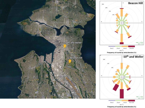
Chemically speciated PM_2.5 data was collected at two Chemical Speciation Network (CSN) sites in Seattle, WA. The Washington State Department of Ecology’s urban National Core multipollutant network site (Beacon Hill, 47.5682 N, 122.3085 W, 102 m a.s.l.) and near-road (10th and Weller, 47.5972 N, 122.3197 W, 42 m a.s.l.) sites are located three and one miles southeast of downtown Seattle, respectively. Beacon Hill is located about half a mile east of Interstate-5 in Seattle’s Beacon Hill neighborhood, while 10th and Weller is located at the intersection of Interstates 5 and 90 in Seattle’s International District. The Washington State Department of Transportation estimated the average daily traffic volume on Interstate-5 (near the 10th and Weller site) in 2017 to be 150,000 vehicles, comprising a significant source of PM_2.5 in the area. Other sources in the Seattle region that may influence the two sites include the Port of Seattle, industry in the south of downtown neighborhood, and local residential wood combustion for home heating. A regional map including both sites is shown in Figure 1. The overall wind profiles at both sites for the 2015–2017 study period are also shown in Figure 1. Both sites experience their strongest winds from the south.

Figure 1. Left: map of Seattle showing the two monitoring site locations. Right: wind roses for Beacon Hill (top) and 10th and Weller (bottom) during the study period.

Data from the Chemical Speciation Network (CSN) were collected for 24 hours every third day at Beacon Hill and every sixth day at 10th and Weller. CSN monitors use polytetrafluoroethylene (PTFE), nylon, and quartz filters to collect PM_2.5 for the offline chemical analysis of metals, ions, and carbon using energy-dispersive X-ray fluorescence, ion chromatography, and thermal optical analysis. Thermal optical analysis of quartz filters allows differentiation of different organic and elemental carbon fractions which aids in source identification. Total organic carbon is equal to the sum of four organic carbon fractions (OC1, OC2, OC3, OC4) and the pyrolized carbon fraction (OP), and total elemental carbon is equal to the sum of three elemental carbon fractions (EC1, EC2, EC3) less the pyrolized carbon fraction (OP) (Solomon et al. 2014).

PMF analysis

PMF analysis utilized EPA’s PMF 5.0 model (https://www.epa.gov/air-research/positive-matrix-factorization-model-environmental-data-analyses). Prior to PMF analysis, CSN data was corrected for field blanks, negative or missing sample values, data completeness, poor signal-to-noise ratios, and any double-counting by similar chemical species, following previous CSN PMF analyses (Kim, Hopke, and Qin 2012; Kotchenruther 2013). Missing uncertainties were also estimated, and special events (i.e., fireworks and wildfires) were excluded from the data. More details about data treatment follow.

CSN data obtained from EPA’s Air Quality System (AQS) is not blank-corrected. Field blank data was also obtained from AQS and when collected simultaneously with sample data the blank concentrations were directly subtracted from the sample concentrations. Samples without an associated field blank utilized the median value from the previous three blank samples.

Missing and negative values are not allowed in the PMF model, as all source contributions are assumed to be positive. Missing data was replaced by the species’ median concentration; the associated sample uncertainty was set to four times the species’ median concentration. Chemical species with data completeness less than 50% were removed from analysis. EPA’s PMF model does not allow negative data and thus negative measurement values that generally occur when a species concentrations is close to zero were set to zero.

Including similar chemical species (i.e., sulfate and sulfur) can bias the PMF solution by over-weighting the contribution of a chemical species to the factor solution. Before analysis, one of the duplicate species was removed to avoid double counting, based on signal-to-noise ratios and data completeness. For this analysis, S, Na⁺, K, Cl, and OP_TOT (OP measured via the Thermal Optical Transmittance method) were retained, while SO₄^2-, Na, K⁺, Cl⁻, and OP_TOR (OP measured via the Thermal Optical Reflectance method) were discarded. Because the organic pyrolysis (OP) concentration is also a portion of the EC1 concentration, EC1 was recalculated and included in PMF analysis as EC1-OP.

CSN datasets include analytical uncertainties associated with sample measurements. The overall measurement uncertainty for each species was calculated using the associated analytical uncertainty as well as the method detection limit (MDL). If a measurement value was below the measurement’s MDL, uncertainty was set to 5/6 of the MDL or the reported uncertainty, whichever was largest. If a measurement value was above the MDL, the uncertainty was set to the reported analytical uncertainty plus 1/3 of the MDL. Missing analytical uncertainties were estimated following Kim et al. (2005). Species were excluded from analysis if their signal-to-noise ratio was less than 0.2.

After data treatment, the remaining species included in PMF analysis with their relevant statistics are listed in the Supplemental Table 1.

PMF modeling followed EPA’s PMF 5.0 Fundamentals and User Guide. Each monitoring site was modeled separately. PMF results were determined to be stable based on bootstrapping and displacement tools available within EPA PMF 5.0. These tools assess random data errors, solution variances, and rotational ambiguity. All factors (200 runs, R = 0.6) were mapped to their original factors 100% of the time at Beacon Hill, aside from diesel exhaust (74%). At 10th & Weller, all factors were mapped to their original factors greater than 90% of the time, aside from gasoline exhaust (89%). Bootstrapping results are shown in the Supplemental Information. No displacement swaps occurred, indicating that significant rotational ambiguity does not exist and that the solution is well constrained. No constraints were applied to either solution.

Results and discussion

Source identification

Sources from PMF analysis were identified based on their association with factor composition, temporal behavior, associated meteorology data, and source profiles from EPA’s SPECIATE database. The following factors were identified at both Beacon Hill and 10th and Weller: wood smoke, sea salt, aged sea salt, residual fuel oil, gasoline exhaust, diesel exhaust, sulfur-rich, nitrate-rich, crustal, and unidentified urban. PMF analysis also identified a factor associated with high zinc concentrations at Beacon Hill. Factor composition is described in detail in section 4, and mass concentration time series as well as chemical profiles are available in the Supplemental Information. Note that the factors associated with gasoline vehicle emissions likely only capture the primary PM_2.5 component of gasoline emissions.

The total factor mass from PMF analysis comprised on average 87% and 86% of the total PM_2.5 from speciation sampling days (excluding fireworks and wildfires) at Beacon Hill and 10th and Weller, respectively. Unaccounted for mass likely represents noise and uncertainty in the measured data and PMF analysis as well as the presence of insignificant sources. Average mass concentrations of collocated Federal Equivalent Method instruments during 2015–2017 were 6.3 µg m⁻³ (±2.1 µg m⁻³) and 8.3 µg m⁻³ (±2.8 µg m⁻³) at Beacon Hill and 10th and Weller, respectively.

The average factor contributions during the study period for both sites are shown in Figure 2 and listed in Table 1. Average concentrations for each factor are shown in the Supplemental Information. While sources were present at both sites, the dominant factors at Beacon Hill were associated with primary gasoline exhaust, unidentified urban, and nitrate-rich factors, while the dominant factors at 10th and Weller were associated with primary diesel and gasoline exhaust factors. Biogenic factors such as crustal and sea salt were similar at both sites. A factor associated with residential wood smoke was also prevalent at both sites.

Table 1. Average factor concentrations (µg m⁻³) during the study period for both sites, with the associated average percentage contribution to total identified sources in parentheses.

Factor	Beacon Hill	10th and Weller
Nitrate-rich	0.45 (14%)	0.39 (8%)
Sulfur-rich	0.28 (9%)	0.38 (8%)
Unidentified Urban	0.51 (16%)	0.18 (4%)
Gasoline	0.92 (26%)	1.03 (21%)
Diesel	0.09 (3%)	1.41 (29%)
Wood Smoke	0.22 (8%)	0.46 (9%)
Crustal	0.28 (8%)	0.47 (10%)
Sea Salt	0.06 (2%)	0.13 (3%)
Aged Sea Salt	0.15 (5%)	0.25 (5%)
Residual Fuel Oil	0.19 (7%)	0.22 (4%)
Zinc-rich	0.06 (2%)	–

Figure 2. Percent contributions to total PM_2.5 by source, as identified at Beacon Hill and 10th and Weller.

Source contributions determined from this study are comparable to those determined in previous source apportionment studies conducted using CSN and IMPROVE data from the past 20 years at the Beacon Hill site (Table 2; Kim and Hopke 2008; Kotchenruther 2013, 2015; Maykut et al. 2003). Specifically, previous determinations of biogenic source contributions (sea salt + aged sea salt + crustal) ranged from 11.3–19% of the total sources; this study determined a total biogenic contribution of 15% of the measured PM_2.5. Contributions to PM_2.5 from wood smoke, nitrate-rich PM_2.5, residual fuel oil, and vehicle emissions are also consistent with previous studies. One exception are the differences in vehicle emissions found in Maykut et al. (2003), which may be due to difficulty resolving the carbon fractions present in the gasoline and diesel factors. However, the total vehicle emissions (22%) is similar to that determined in this study (29%). Maykut et al. (2003) and Kim and Hopke (2008) also utilized CSN data prior to EPA’s analytical methodology change in 2007 to OC and EC determinations; changes in methodology may also bias comparisons (Spada and Hyslop 2018).

Table 2. Comparison of source contributions at Beacon Hill by study and years of data included.

	Maykut et al. 2003	Kim and Hopke 2008	Kotchenruther 2013	Kotchenruther 2015	Kotchenruther 2015	This analysis
Study Years	1996–1999	2000–2005	2007–2011	2006–2009	2009–2013	2015–2017
Biogenic	17%	11%	20%	14%	14%	15%
Nitrate-rich/secondary nitrate	–	18%	9%	17%	14%	14%
Wood Smoke	–	8%	11%	16%	16%	8%
Residual Fuel Oil	10%	6%	15%	7%	10%	7%
Gasoline Exhaust	4%	31%	20%	26%	29%	26%
Diesel Exhaust	18%	5%	–	–	–	3%
Metals	–	2%	12%	3%	2%	2%
Sulfate-rich/secondary sulfate	18%	18%	–	15%	14%	9%
Unidentified Urban	–	–	9%	–	–	16%

Note: Biogenic = (sea salt + aged sea salt + crustal).

This study is the first reported source apportionment analysis of PM_2.5 speciation data at the 10th and Weller near-road site. However, a community toxics study by Puget Sound Clean Air Agency in 2016 (Puget Sound Clean Air Agency 2018) conducted PMF on 61 days of 24-hour air toxics data to estimate an annual average diesel PM_2.5 concentration of 1.4–1.7 µg m⁻³. Similar to this study, Puget Sound Clean Air Agency found diesel PM_2.5 mixed with other factors, leading to difficulty estimating a single concentration for diesel PM_2.5 at the site. This study estimates an average diesel PM_2.5 concentration of 1.4 µg m⁻³. Given the presence of diesel chemical components in other factors (i.e., elemental carbon in sea salt), we also assume the diesel PM_2.5 concentration as a lower limit of total diesel PM_2.5 exposure at 10th and Weller.

Annual contributions

Annual factor contributions at both sites (Figure 3) show that PM_2.5 associated with gasoline exhaust has increased while the contribution associated with residual fuel oil combustion has decreased from 2015–2017. The decrease in residual fuel oil combustion is due to changes in marine high-sulfur fuel regulations; previous studies have observed the decreasing trend in PM_2.5 emissions from marine vessels (Kotchenruther 2015; Spada et al. 2018). PM_2.5 from diesel exhaust has not changed significantly at either site, suggesting no volume changes in diesel vehicles on the highways. This is corroborated by WSDOT traffic data near the 10th and Weller site which shows similar annual average vehicle volumes from 2015 to 2017.

Figure 3. Annual factor contributions at Beacon Hill (left) and 10th and Weller (right).

That the percent contribution from gasoline vehicles to total PM_2.5 at both sites increases over the three-year period suggests potential increases in vehicle volumes across all road types or increases in emission factors due to increasing congestion. However, without more data points to add to the three-year period, it is also plausible that the increases in gasoline exhaust emissions is due to variability in meteorology. While 10th and Weller is closer to the Interstate than Beacon Hill, both monitoring sites are impacted by residential and commercial traffic on local roads. The impact of the freeway is clearly observed in the higher concentration of diesel PM_2.5 at 10th and Weller. However, given that gasoline PM_2.5 is similar at Beacon Hill and 10th and Weller, it is likely that the gasoline source is from all road types and cannot be isolated only to the freeway. A recent study examining long-term trends of source apportioned PM_2.5 also found that the contribution from spark-ignition vehicles is also increasing, consistent with the number of registered vehicles in New York State (Masoil et al. 2019).

Trend analysis utilizing Theil-Sen methods identifies significant decreasing patterns at both sites for residual fuel oil, nitrate-rich, unidentified urban (p-values less than 0.05). As only three years of data are included in this analysis, patterns over time should be interpreted with caution. Specifically, residual fuel oil PM_2.5, nitrate-rich PM_2.5, and unidentified urban PM_2.5 is decreasing on average 0.1, 0.08, and 0.1 µg m⁻³ per year. PM_2.5 from gasoline emissions show a significant increasing trend of 0.18 µg m⁻³ per year at both sites (p-value < 0.05), while the trend for diesel PM_2.5 is only significant at the Beacon Hill site (0.02 µg m⁻³ per year, p-value < 0.01). That the total observed PM_2.5 shows no significant patterns at each site is largely due to individual sources of PM_2.5 balancing each other over time.

Seasonal concentrations

Seasonal concentrations of each factor are shown in Figure 4 for both sites. The heating season is defined as September 21 thru March 20, while the non-heating season includes the remaining months. Seasonal concentrations show that wood smoke at both sites has a significantly higher contribution to the total PM_2.5 mass during the heating season, when temperatures are colder and residential heating is more prevalent (Figure 4). The nitrate-rich factor is also higher in the fall and winter, when low temperatures and high relative humidity favor the formation of secondary nitrate particles (Seinfeld and Pandis 2006). Higher concentrations of PM_2.5 associated with gasoline emissions during colder months suggests a potential increase in cold-starts from vehicles (Kittelson et al. 2006; Zhao et al. 2018). That this increase is not observed in the diesel factor suggests that an increase in cold-starts is isolated to gasoline vehicles as potentially diesel vehicles are more likely to pass through the city on the interstates. Similarities in the PMF chemical profiles of gasoline and wood smoke factors also may impact the seasonality of gasoline emissions – organic carbon fractions significantly contribute to both gasoline and wood smoke factors. Sulfur-rich PM_2.5 concentrations are larger in the summer, likely due to increased photochemistry. Seasonal concentration differences may also be due to differences in boundary layer heights between summer and winter.

Figure 4. Seasonal concentrations of each factor at Beacon Hill and 10th and Weller. The heating season includes fall and winter, while the non-heating season includes spring and summer. Error bars are the standard deviation of the mean.

The presence of a factor associated with wood smoke at the near-road 10th and Weller site is corroborated by Puget Sound Clean Air Agency’s 2016 toxics study at 10th and Weller that also found a contribution from wood smoke (Puget Sound Clean Air Agency 2018). The wood smoke PM_2.5 observed at 10th and Weller most likely originated from nearby residential neighborhoods, which are located mainly to the east of the site (Supplemental Information).

Weekday/weekend effects

PM_2.5 associated with diesel emissions at 10th and Weller exhibited no significant seasonal or yearly differences but did show a weekday/weekend effect (Figure 5). Less diesel PM_2.5 emissions occur on weekend days likely due to decreases in work-related diesel truck traffic. This is evident in the 10th and Weller data, likely due to the close proximity of the highways. However, there was no difference between weekday and weekend concentrations of diesel PM_2.5 at the Beacon Hill site, which is not as close to the highways and also exhibits much lower diesel PM_2.5 concentrations – any changes in concentration magnitude may be difficult to discern.

Figure 5. Weekend and weekday concentrations of factors at Beacon Hill and 10th and Weller. Error bars are one standard deviation of the mean.

PM_2.5 at Beacon Hill associated with crustal emissions also showed a difference in weekday concentrations compared to weekend concentrations. Given that crustal PM_2.5 concentrations are low (0.28 µg m⁻³), this difference may be due to noise in the data rather than differences in emissions. No other factors showed a distinction between weekdays and weekends.

Detailed factor descriptions

Diesel

PM_2.5 associated with diesel emissions accounted for only 3% of total PM_2.5 at Beacon Hill, but 29% of total PM_2.5 at 10th and Weller. Diesel PM_2.5 is dominated by elemental carbon fractions (EC1 and EC2), and is fairly consistent throughout seasons. The highest concentrations of the diesel factor at Beacon Hill were observed from the south and to the west, which both indicate influence from Interstate-5. The highest concentrations of the diesel factor observed at 10th and Weller are from the directions of Interstates 5 and 90. However, it is likely that the factor’s directionality is biased by the prevailing winds, given that wind data is averaged to 24 hours to match the 24-hour integrated chemical samples.

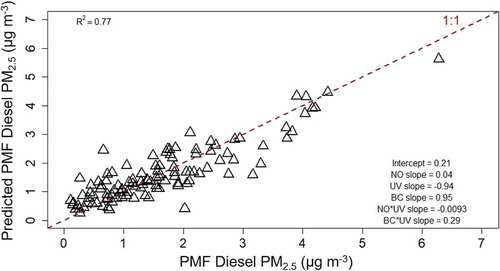
The 10th and Weller monitoring site also houses instruments measuring nitrogen oxides and black carbon. Correlations between the diesel factor determined by PMF and these ancillary measurements are shown in Figure 6 and suggest diesel PM_2.5 can be traced by existing measurements at 10th and Weller. To further test that theory, predicted diesel PM_2.5 was modeled utilizing Nitrogen Monoxide (NO) and aethelometer carbon measurements. The aethelometer determines Black Carbon (BC) and UV-light absorbing carbon (UV) mass concentrations from the changes in optical attenuations at 880 nm and 370 nm, respectively. The model using UV, BC, and NO predicts PMF diesel PM_2.5 better than using only BC or NO concentrations, with an R² of 0.77 (Figure 7). Specifically, a linear regression models predicted PMF diesel PM_2.5 as equal to: a + bNO + cUV + dBC + eNO*UV + fUV*BC; where a = 0.21; b = 0.04; c = − 0.94; d = 0.95; e = − 0.0093; and f = 0.29.

Figure 6. PMF diesel PM_2.5 concentrations as a function of NO (left) and black carbon (right), with the linear regression line shown in red. Correlation coefficients for NO and BC are 0.6 and 0.46, respectively.

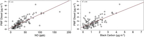
Figure 7. A simple model utilizing NO, UV, and BC predicted 24-hour concentrations of diesel PM_2.5, and is compared to diesel PM_2.5 determined by PMF analysis, with the 1:1 line in red. Predicted PMF diesel PM_2.5 = a + bNO + cUV + dBC + eNO*UV + fUV*BC; where a = 0.21; b = 0.04; c = − 0.94; d = 0.95;e = 0.0093; and f = 0.29.

The predictive model was tested using daily averages of NO, UV, and BC to predict diesel PM_2.5 concentrations more often than the CSN sampling schedule of every six days. On average, predicted daily diesel PM_2.5 is 20% of measured daily PM_2.5 from November 2014 – December 2018. The PMF Diesel factor accounted for 29% of total PM_2.5 at 10th and Weller, yet the PM_2.5 captured by PMF was only 86% of the total measured PM_2.5. Accounting for the missing PM_2.5 mass increases the estimated daily diesel PM_2.5 percentage to 23% of the total measured PM_2.5.

The predictive model was further utilized to estimate diesel PM_2.5 concentrations on an hourly timescale. Figure 8 shows hourly averages of the ratio of predicted diesel to hourly measured PM_2.5 as a function of PM_2.5 concentrations split into concentration bins ranging from 0–5 µg m⁻³ to greater than 100 µg m⁻³. Diesel PM_2.5 comprises about 20% of the total PM_2.5 across the range of PM_2.5 concentration bins. This indicates that on average 10th and Weller has a background concentration of diesel PM_2.5 that is about 20% of the total measured PM_2.5. The correlation between diesel PM_2.5 and NO at Beacon Hill was also investigated, and is shown in the Supplemental Information. The very low correlation (R² = 0.03) suggests that diesel PM_2.5 is most easily modeled and predicted in environments subject to high diesel PM_2.5 concentrations.

Figure 8. Average hourly predicted diesel PM_2.5 (µg m^-3) as a function of measured PM_2.5 (µg m^-3) 2014–2018.

The predictive model was also applied to near-road sites across the country that also measure NO, BC, and UV concentrations. Note that this exercise is largely illustrative of how diesel PM_2.5 can be assessed without a full chemical speciation analysis. The predictive model is likely site-specific and dependent on the mixture of gasoline and diesel vehicles. NO_x concentrations at each site will also be dependent on ozone concentrations and the extent of ozone titration by NO. However, the predictive model can be qualitatively utilized to motivate comparisons between PM_2.5 sources and continuous measurements at monitoring sites. Figure 9 shows that the ratio of predicted diesel PM_2.5 to measured PM_2.5 scales with roadways observing high traffic concentrations. The ratio of predicted diesel PM_2.5 to measured PM_2.5 was also highest for sites closer to their target roads, indicating that diesel PM_2.5 exposure can be reduced by increasing one’s distance from a major roadway.

Figure 9. Distance from target road (m) as a function of annual average daily traffic for near-road sites across the United States that measure inputs to the predictive model shown in Figure 7. Colors indicate the estimated contribution of diesel PM_2.5 to the total PM_2.5 measured.

Gasoline

The PM_2.5 factor associated with primary gasoline exhaust emissions accounted for about 26% of the PM_2.5 at Beacon Hill and 21% of the PM_2.5 at 10th and Weller. The source profile for gasoline is characterized by a 1:2:1 ratio between the organic carbon fractions OC2, OC3, and OC4. EC1 is about 15% of the total gasoline factor at Beacon Hill, consistent with previous PMF analyses (Kotchenruther 2013). On the other hand, EC1 at 10th and Weller contributes less than 1% to the factor composition, suggesting that the diesel and gasoline factors were difficult to separate at 10th and Weller given the high concentration of EC1 in the diesel factor. Meteorology data at both sites indicates the source of gasoline is both from local and from the direction of the freeways. Slight seasonality is observed, with higher gasoline concentrations during the fall. The factor composition also includes small contributions from elements found in tire and brake wear profiles, including copper, chromium, and iron (Hjortenkrans, Bergback, and Haggerud 2007; Lough et al. 2005).

Wood smoke

PM_2.5 associated with wood smoke is characterized by a dominant OC1 peak and about 1% potassium and 20% EC1. Wood smoke concentrations also are highest during the colder months, and the factor accounts for about 7% and 9% of the total PM_2.5 at Beacon Hill and 10th and Weller, respectively. The potassium to OC ratios in the average wood smoke profile from both sites (0.012 and 0.086) are similar to previous ratios reported (Kotchenruther 2016; Munchak et al. 2011). Wood smoke concentrations at Beacon Hill and 10th and Weller are likely coming from similar neighborhoods, as the pollution roses (Supplemental Information) indicate the highest concentrations of wood smoke likely reflect local neighborhood home heating during colder temperatures.

Residual fuel oil

Dominated by nitrate, sulfur, and ammonium, residual fuel oil contributed 6% and 5% to the total PMF PM_2.5 at Beacon Hill and 10th and Weller, respectively. However, temporal trends at both sites indicate a decrease in the factor over time. Organic carbon fractions and nickel were also present in the factor composition, consistent with previous studies (Kotchenruther 2013, 2015). While not utilized in the PMF analysis due to a high signal-to-noise ratio, vanadium was also present concurrent with high concentrations of the residual fuel oil factor. The vanadium to nickel ratio has previously been used to confirm the identity of the residual fuel oil factor; Kotchenruther (2013) identified a ratio of 2.4–3.9 and Cesari et al. (2014) identified a ratio of 1.7. The vanadium to nickel ratio mean during high concentrations of the residual fuel oil factor in this study was 1.7 (±1). The strong presence of nitrate is unusual in previously identified residual fuel oil emissions profiles (i.e., EPA’s SPECIATE database), and may indicate a mixture of fuel oil with secondary nitrate components. Future studies should attempt to delineate these two sources. Meteorology at the Beacon Hill site indicates high concentrations are from the northeast and northwest. The Port of Seattle is located slightly to the northwest of the Beacon Hill site and slightly to the southwest of the 10th and Weller site. Meteorology at the 10th and Weller site indicates highest concentrations from the south, with contributions from all directions. Pollution roses for both sites are shown in the supplemental information. Factor composition at 10th and Weller also shows a higher contribution from elemental carbon than at Beacon Hill, which is reflective of 10th and Weller’s location next to I-5 and the prevalence of diesel PM_2.5 at the site.

Nitrate-rich

Nitrate-rich PM_2.5 (PM_2.5 associated with high concentrations of nitrate) comprises 14% and 8% of the total PM_2.5 at Beacon Hill and 10th and Weller, respectively, and is dominated by NO₃⁻. Ammonium was only a small fraction of the total factor mass, suggesting the nitrate-rich PM_2.5 is not all secondary or was difficult to separate from the high ammonium and nitrate concentrations in the residual fuel oil factor. However, the factor is higher in the winter than the summer, consistent with secondary nitrate, as low temperatures and high relative humidity favor higher ammonium nitrate aerosol concentrations. The presence of potassium in this factor also may indicate a link between nitrate-rich PM_2.5 and wood burning. Primary sources of nitrogen oxides include fuel combustion, soils, and biomass burning.

Sulfur-rich

Sulfur-rich PM_2.5 (PM_2.5 associated with high concentrations of sulfur) comprised 9% and 8% of the total PM_2.5 at Beacon Hill and 10th and Weller, respectively, and is dominated by S. Similar to nitrate-rich PM_2.5, ammonium was only a small fraction of the total factor mass. However, the temporal behavior and seasonality of the sulfur-rich factor is consistent with secondary sulfate, as the sulfur-rich factor is higher in the summer due to increased photochemical activity. Reaction pathways that favor secondary sulfate also may lead to the formation of secondary organic aerosol, which potentially explains the percentage of organic carbon components in the sulfur-rich factor. This factor also potentially includes influences from the residual fuel oil factor, as small concentrations of nickel are present in the sulfur-rich factor. Further, pollution roses point to a high concentration of the sulfur-rich factor coming from the direction of the Port of Seattle (Supplemental Information). It is likely that the sulfur-rich factor is representing a mixture of sulfur-emitting sources in the Seattle area, including residual fuel oil combustion.

Unidentified urban

Unidentified Urban accounts for 16% and 4% of the total PM_2.5 at Beacon Hill and 10th and Weller, respectively. Factor composition is consistent with previous identifications that link this factor with secondary PM_2.5 formation as well as fuel combustion activities (Kotchenruther 2013). Previous studies have also linked the components in this factor to a mixture of secondary PM_2.5 and wood smoke due to the presence of organic carbon and pyrolysis components as well as potassium (Kotchenruther 2016). No seasonal trends are observed, and meteorology suggests the factor source is from downtown, industrial, and local neighborhoods.

Crustal

PM_2.5 associated with crustal emissions (also called fugitive dust) contains elements commonly found in soils, including aluminum, calcium, iron, manganese, and silicon, and accounts for 9% of the total PM_2.5 at Beacon Hill and 10% of the total PM_2.5 at 10th and Weller.

Sea salt

Sea salt PM_2.5 is dominated by chlorine, with contributions from sodium and magnesium as well. Concentrations are fairly low on average, with occasional concentration spikes. Wind direction shows the highest concentrations of sea salt PM_2.5 from south of the Beacon Hill site and southwest of the 10th and Weller site.

Aged sea salt

Aged sea salt is similar in composition to sea salt, except nitrate has displaced chloride, consistent with aged sea salt identification (Kim and Hopke 2008). The sources of aged sea salt at both sites is from all directions, consistent with the aged nature of the factor.

Zinc-rich

A factor associated with high zinc concentrations was only found at Beacon Hill, and is characterized by a high zinc concentration, comprising 11% of the total factor mass. Nitrate and organic carbon fractions were also present in the factor composition. Factor concentrations are low, accounting for only 2% of the total PM_2.5 at Beacon Hill. Wind direction analysis suggest the source is primarily local, and potentially from diesel vehicles and industrial activities (Kotchenruther 2013).

Conclusion

Analysis of speciated PM_2.5 measurements by PMF determined that Beacon Hill and 10th and Weller monitoring sites observe similar PM_2.5 sources. Highest contributing sources at both sites include sources associated with vehicle emissions, wood smoke, and secondary PM_2.5. However, the magnitude of sources differ, primarily in the diesel PM_2.5 concentration, which is 15x higher at 10th and Weller compared to Beacon Hill. The location of the sites largely explains the variation in diesel emissions – 10th and Weller is located much closer to the freeways than Beacon Hill and previous studies suggest moving away from the freeways dramatically decreases diesel PM_2.5 exposure (Puget Sound Clean Air Agency 2018).

The diesel PMF factor concentration correlates well with black carbon and nitrogen monoxide measurements at 10th and Weller, indicating diesel PM_2.5 can be traced without a full chemical speciation data analysis. A simple predictive model estimates diesel PM_2.5 contributes about 20% to the total measured PM_2.5 at 10th and Weller. The diesel PMF factor concentration at Beacon Hill was not well correlated with nitrogen oxide measurements, suggesting that diesel PM_2.5 is most easily modeled with the inputs described in Section 4.1 in environments subject to high diesel PM_2.5 concentrations.

Comparison to previous source apportionment studies at Beacon Hill indicate PM_2.5 sources in the Seattle region are largely unchanged over the past 15 years, with the exception of the decrease of residual fuel oil emissions, consistent with recent changes in policy, and an increase in PM_2.5 from gasoline vehicle emissions. Patterns in source concentrations from 2015–2017 indicate significant decreases in PM_2.5 sources associated with residual fuel oil PM_2.5, nitrate-rich PM_2.5, and unidentified urban PM_2.5, and a significant increase in PM_2.5 sources associated with gasoline vehicle emissions.

Disclosure statement

No potential conflict of interest was reported by the author.

Additional information

Notes on contributors

Beth Friedman

Beth Friedman is an air quality scientist at the Washington State Department of Ecology.

References

- Apte, J. S., M. Brauer, A. J. Cohen, M. Ezzati, and C. A. Pope. 2018. Ambient PM2.5 reduces global and regional life expectancy. Environ. Sci. Tech. Let. 5 (9):546–51. doi:10.1021/acs.estlett.8b00360.
- Atkinson, R. W., I. C. Mills, H. A. Walton, and H. R. Anderson. 2015. Fine particle components and health—a systematic review and meta-analysis of epidemiological time series studies of daily mortality and hospital admissions. J. Expo. Sci. Environ. Epidemiol. 25 (2):208–14. doi:10.1038/jes.2014.63.
- Atkinson, R. W., S. Kang, H. R. Anderson, C. Mills, and H. A. Walton. 2014. Epidemiological time series studies of PM2.5 and daily mortality and hospital admissions: A systematic review and meta-analysis. Thorax 69 (7):660–65. doi:10.1136/thoraxjnl-2013-204492.
- Belis, C. A., D. Pernigotti, F. Karagulian, G. Pirovano, B. R. Larsen, M. Gerboles, and P. K. Hopke. 2015. A new methodology to assess the performance and uncertainty of source apportionment models in intercomparison exercises. Atmos. Environ. 119:35–44. doi:10.1016/j.atmosenv.2015.08.002.
- Brook, R. D., S. Rajagopalan, C. A. Pope III, J. R. Brook, A. Bhatnagar, A. V. Diez-Roux, F. Holguin, Y. Hong, R. V. Luepker, M. A. Mittleman et al. 2010. Particulate matter air pollution and cardiovascular disease. Circulation. 121(21):2331–78. doi:10.1161/CIR.0b013e3181dbece1.
- Brunekreef, B., and S. T. Holgate. 2002. Air pollution and health. Lancet 360 (9341):1233–42. doi:10.1016/S0140-6736(02)11274-8.
- Cesari, D., A. Genga, P. Ielpo, M. Siciliano, G. Mascolo, F. M. Grasso, and D. Contini. 2014. Source apportionment of PM2.5 in the harbor-industrial area of Brindisi (Italy): Identification and estimation fo the contribution of in-port ship emissions. Sci. Total Environ. 497–498:392–400. doi:10.1016/j.scitotenv.2014.08.007.
- Guarnieri, M., and J. R. Balmes. 2014. Outdoor air pollution and asthma. Lancet 383 (9928):1581–92. doi:10.1016/S0140-6736(14)60617-6.
- Hjortenkrans, D. S. T., B. G. Bergback, and A. V. Haggerud. 2007. Metal Emissions from Brake Linings and Tires: Case Studies of Stockholm, Sweden 1995/1998 and 2005. Environ. Sci. Technol. 41 (15):5224–30. doi:10.1021/es070198o.
- Hopke, P. K. 2016. Review of Receptor Modeling Methods for Source Apportionment. J. Air Waste Manage. Assoc. 66 (3):237–59. doi:10.1080/10962247.2016.1140693.
- Janssen, N. A. H., G. Hoek, M. Simic-Lawson, P. Fischer, L. van Bree, H. Ten Brink, M. Keuken, R. W. Atkinson, H. R. Anderson, B. Brunekreef, et al. 2011. Black Carbon as an Additional Indicator of the Adverse Health Effects of Airborne Particles Compared with PM10 and PM2.5. Environ. Health Perspect. 119:12. doi:10.1289/ehp.1003369.
- Kampa, M., and E. Castanas. 2008. Human health effects of air pollution. Environ. Pollut. 151 (2):362–67. doi:10.1016/j.envpol.2007.06.012.
- Kim, E., and P. K. Hopke. 2008. Source characterization of ambient fine particles at multiple sites in the Seattle area. Atmos. Environ. 42 (24):6047–56. doi:10.1016/j.atmosenv.2008.03.032.
- Kim, E., P. K. Hopke, and Y. Qin. 2005. Estimation of organic carbon blank values and error structures of the speciation trends network data for source apportionment. J. Air Waste Manage. Assoc. 55 (8).
- Kim, E., P. K. Hopke, and Y. Qin. 2012. Estimation of organic carbon blank values and error structures of the speciation trends network data for source apportionment. J. Air Waste Manage. Assoc. 55 (8):1190–99. doi:10.1080/10473289.2005.10464705.
- Kittelson, D. B., W. F. Watts, J. P. Johnson, J. J. Schauer, and D. R. Lawson. 2006. On-road and laboratory evaluation of combustion aerosols—Part 2:: Summary of spark ignition engine results. J. Aerosol. Sci. 37 (8):931–49. doi:10.1016/j.jaerosci.2005.08.008.
- Kotchenruther, R. A. 2013. A regional assessment of marine vessel PM2.5 impacts in the U.S. Pacific Northwest using a receptor-based source apportionment method. Atmos. Environ. 68:103–11. doi:10.1016/j.atmosenv.2012.11.067.
- Kotchenruther, R. A. 2015. The effects of marine vessel fuel sulfur regulations on ambient PM2.5 along the west coast of the U.S. Atmos. Environ. 103:121–28. doi:10.1016/j.atmosenv.2014.12.040.
- Kotchenruther, R. A. 2016. Source apportionment of PM2.5 at multiple Northwest U.S. sites: Assessing regional winter wood smoke impacts from residential wood combustion. Atmos. Environ. 142:210–19. doi:10.1016/j.atmosenv.2016.07.048.
- Lough, G. C., J. J. Schauer, J.-S. Park, M. M. Shafer, J. T. DeMinter, and J. P. Weinstein. 2005. Emissions of Metals Associated with Motor Vehicle Roadways. Environ. Sci. Technol. 39 (3):826–36. doi:10.1021/es048715f.
- Masoil, M., S. Squizzato, D. Q. Rich, and P. K. Hopke. 2019. Long-term trends (2005-2016) of source apportioned PM2.5 across New York State. Atmos. Environ. 201 (15):110–20. doi:10.1016/j.atmosenv.2018.12.038.
- Maykut, N. N., J. Lewtas, E. Kim, and T. V. Larson. 2003. Source Apportionment of PM2.5 at an Urban IMPROVE Site in Seattle, Washington. Environ. Sci. Technol. 37 (22):5135–42. doi:10.1021/es030370y.
- Munchak, L. A., B. A. Schichtel, A. P. Sullivan, A. S. Holden, S. M. Kreidenweis, W. C. Malm, and J. L. Collett Jr.. 2011. Development of wildland fire particulate smoke marker to organic carbon emission ratios for the conterminous United States. Atmos. Environ. 45 (2):395–403. doi:10.1016/j.atmosenv.2010.10.006.
- Paatero, P. 1997. Least squares formulation of robust non-negative factor analysis. Chemometr. Intell. Lab. 37 (1):23–35. doi:10.1016/S0169-7439(96)00044-5.
- Paatero, P., and P. K. Hopke. 2003. Discarding or Downweighing High-Noise Variables in Factor Analysis Models. Analytica. Chimica. Acta. 490 (1–2):277–89. doi:10.1016/S0003-2670(02)01643-4.
- Paatero, P., and U. Tapper. 1994. Positive matrix factorization: A non-negative factor model with optimal utilization of error estimates of data values. Environmetrics 5 (2):111–26. doi:10.1002/env.3170050203.
- Pope, C. A., and D. W. Dockery. 2006. Health effects of fine particulate air pollution: Lines that connect. J. Air Waste Manage. Assoc. 56 (6). doi: 10.1080/10473289.2006.10464485.
- Puget Sound Clean Air Agency. 2018. Near-road air toxics study in the Chinatown-International District. http://www.pscleanair.org/DocumentCenter/View/3397/Air-Toxics-Study-in-the-Chinatown-International-District-Reduced.
- Reff, A., S. I. Eberly, and P. V. Bhave. 2007. Receptor modeling of ambient particulate matter data using positive matrix factoriation: Review of existing methods. J. Air Waste Manage. Assoc. 57 (2):146–54. doi:10.1080/10473289.2007.10465319.
- Seinfeld, J. H., and S. N. Pandis. 2006. Atmospheric chemistry and physics: From air pollution to climate change. 2nd ed. Wiley-Interscience.
- Solomon, P. A., D. Crumpler, J. B. Flanagan, R. K. M. Jayanty, E. E. Rickman, and C. E. McDade. 2014. U.S. National PM2.5 chemical speciation monitoring networks—CSN and IMPROVE: Description of networks. J. Air Waste Manage. Assoc. 64 (12):1410–38. doi:10.1080/10962247.2014.956904.
- Song, C., J. He, L. Wu, T. Jin, X. Chen, R. Li, P. Ren, L. Zhang, and H. Mao. 2017. Health burden attributable to ambient PM2.5 in China. Environ. Pollut. 223:575–86. doi:10.1016/j.envpol.2017.01.060.
- Spada, N. J., and N. P. Hyslop. 2018. Comparison of elemental and organic carbon measuremnets between IMPROVE and CSN before and after method transitions. Atmos. Environ. 178:173–80. doi:10.1016/j.atmosenv.2018.01.043.
- Spada, N. J., X. Cheng, W. H. White, and N. P. Hyslop. 2018. Decreasing Vanadium footprint of bunker fuel emissions. Environ. Sci. Technol. 52 (20):11528–34. doi:10.1021/acs.est.8b02942.
- Wu, C., T. V. Larson, S. Wu, J. Williamson, H. H. Westberg, and L.-J. S. Liu. 2007. Source apportionment of PM2.5 and selected hazardous air pollutants in Seattle. Science of the Total Environ. 386 (1–3):42–52. doi:10.1016/j.scitotenv.2007.07.042
- Zhao, Y., A. T. Lambe, R. Saleh, G. Saliba, and A. L. Robinson. 2018. Secondary organic aerosol production from gasoline vehicle exhaust: effects of engine technology, cold start, and emission certification standard. Environ. Sci. Technol. 52 (3):1253–61. doi:10.1021/acs.est.7b05045.