The Comprehensive Fire Information Reconciled Emissions (CFIRE) inventory: Wildland fire emissions developed for the 2011 and 2014 U.S. National Emissions Inventory

ABSTRACT

Wildland fire emissions from both wildfires and prescribed fires represent a major component of overall U.S. emissions. Obtaining an accurate, time-resolved inventory of these emissions is important for many purposes, including to account for emissions of greenhouse gases and short-lived climate forcers, as well as to model air quality for health, regulatory, and planning purposes. For the U.S. Environmental Protection Agency’s 2011 and 2014 National Emissions Inventories, a new methodology was developed to reconcile the wide range of available fire information sources into a single coherent inventory. The Comprehensive Fire Information Reconciled Emissions (CFIRE) inventory effort utilized satellite fire detections as well as a large number of national, state, tribal, and local databases. The methodology and results for CONUS and Alaska were documented and compared against other fire emissions databases, and the efficacy of the overall effort was evaluated. Results show the overall spatial pattern differences and relative seasonality of wildfires and prescribed fires across the country. Prescribed burn emissions occurred primarily in non-summer months were concentrated in the Southeast, Northwest, and lower Midwest, and were relatively consistent year to year. Wildfire emissions were much more variable but occurred primarily in the summer and fall. Overall, CFIRE represents a third of total emitted PM2.5 across all sources in the National Emissions Inventory, with prescribed fires accounting for nearly half of all CFIRE emissions. Compared with other wildland fire emissions inventories derived solely from satellite detections, the CFIRE inventory shows markedly increased emissions, reflecting the importance of the multiple national and regional databases included in CFIRE in capturing small fires and prescribed fires in particular.

Implications: Wildland fire emissions inventories need to incorporate multiple sources of fire information in order to better represent the full range of fire activity, including prescribed burns and smaller fires. For the 2011 and 2014 U.S. National Emissions Inventory, a methodology was developed to collect, associate, and reconcile fire information from satellite data as well as a large number of national, regional, state, local, and tribal fire information databases across the country. The resulting emissions inventory shows the importance of this type of integration and reconciliation when compared against other emissions inventories for the same period.

Introduction

Emissions from wildland fires, including wildfires and prescribed fires (planned, human-initiated fires for land management objectives), contain gaseous and particulate species of relevance to global climate and regional air quality. Wildland fires are a significant contributor to global emissions of carbon dioxide (CO₂) and other greenhouse gases, including the short-lived climate forcers like black carbon (BC) (Andreae and Merlet, 2001; Crutzen and Andreae 1990; EPA 2012; Val Martín et al. 2006). Wildland fire smoke contributes directly to exceedances of the U.S. Clean Air Act’s National Ambient Air Quality Standards (NAAQS) due to amount emitted of fine particulate matter (less than 2.5 microns, PM2.5) (e.g. EPA 2012, 2013, 2018), as well as oxides of nitrogen (NOx) and volatile organic compounds (VOCs) that are precursors to ozone (O3) (e.g. Dreessen, Sullivan, and Delgado 2016). Wildland fire smoke can also contain hazardous toxic air pollutants (HAPs) such as acrolein (Crutzen et al. 1990; Urbanski, Hao, and Baker 2008; Wotawa and Trainer 2000). Exposure to smoke from wildland fires is linked to several health issues, including respiratory and cardiovascular impacts (Reid et al. 2016). Overall, wildland fires represent a significant fraction of the total emissions of PM2.5, both globally and in the United States (Dentener et al. 2006).

As such, development of high-quality emissions inventories for wildland fire is important to understand both global climate effects as well as regional and local air quality. Emissions inventories drive global and regional modeling used for scientific, planning, and regulatory purposes. An important inventory, particularly for regulatory and planning purposes, is the U.S. Environmental Protection Agency’s (EPA) National Emissions Inventory (NEI), a comprehensive U.S. inventory produced every three years, including the years 2011 and 2014, which will be focused upon here (EPA 2013, 2018). The EPA uses the NEI for many purposes, including providing input for air quality and risk modeling, assessing regulatory impact, and planning ambient monitoring network locations. Due to the magnitude of wildland fire emissions, considerable effort was made to improve the wildland fire portion of the NEI beginning with the 2011 and 2014 NEIs.

The efforts to improve the 2011 and 2014 wildland fire emissions inventories were undertaken because significant discrepancies exist between different estimates of wildland fire emissions (e.g. Larkin, Raffuse, and Strand 2014). A large portion of these differences are due to differences in how fire activity (e.g. total burned area) information is gathered and used (Drury et al. 2014, 2014; Larkin et al. 2012). Currently, no definitive source exists for fire activity information, particularly for small and/or prescribed fires. Additionally, weaknesses in the wildfire emissions inventory have been identified as an issue for the overall NEI (e.g., Day et al. 2019). To overcome this, a new and substantial effort was undertaken as part of the development of the 2011 and 2014 NEIs to gather all available wildland fire data sources and combine them, with the goal of incorporating more fires than would be possible otherwise. This paper describes these efforts, with particular emphasis on the processing done nationally to incorporate and reconcile a wide range of fire information datasets.

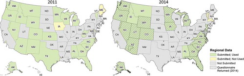
Fire information was gathered from satellites, national reporting systems, and regional databases from state, local, and tribal agencies. Requests for data were made to all U.S. states and through the states to local and tribal agencies, through a process developed as part of the 2011 inventory. For the 2014 inventory, an additional questionnaire was developed and added to the request; this questionnaire was specifically targeted to clarify issues around completeness and inclusiveness of the gathered datasets. Figure 1 shows the locations of the regional databases gathered for each inventory effort.

Figure 1. Regional fire activity datasets used in the 2011 and 2014 National Emissions Inventory wildland fire national processing efforts

The processing and integration of these databases required substantial effort to avoid double counting of fires that appear in more than one dataset. Once integrated, the resulting combined fire information set was sent through a standardized modeling sequence to calculate fuel consumption and emissions. These nationally processed data are presented here; for the final NEI, individual states retained the right to submit their own calculations using any method. Because of these methodological changes, differences in state-submitted methodologies make comparisons between states difficult. For this reason, the nationally processed wildland fire emissions inventory, created through a national effort to gather and reconcile fire information and calculate emissions, is presented and discussed here instead of in the final NEI. Here this emissions inventory is designated as the Comprehensive Fire Information Reconciliation Emissions (CFIRE) inventory to distinguish it from the final official National Emissions Inventory, which included direct state submissions as well. However, the differences between these inventories are minor (see Section 5.2). Only two states each in 2011 (Georgia and North Carolina) and 2014 (Georgia and Washington) submitted their own emissions calculations that were subsequently used in the NEI.

The overall processing, data, models, and methods for the CFIRE inventory are presented in Section 2. Development of the inventories is discussed in Section 3, with particular focus on how the fire information was processed and integrated. Results for both the 2011 and 2014 inventories are shown in Section 4. Comparison with other inventories and methods is discussed in Section 5. Conclusions and lessons learned for future efforts are given in Section 6.

Datasets and models

Overview

For the CFIRE inventory, emissions were computed based on fire activity data for both wildfires and prescribed fires that were collected from all 50 states and Puerto Rico in 2011 and 2014. Because Hawaii and Puerto Rico required a modified methodology due to missing model inputs, only results for the contiguous 48 states and Alaska are presented here.

A starting point for understanding the information needed for calculating emissions for wildland fire can be found in Seiler and Crutzen (1980):

(1) $\mathrm{E}\mathrm{m}\mathrm{i}\mathrm{s}\mathrm{s}\mathrm{i}\mathrm{o}{\mathrm{n}}_i=A\times B\times \mathrm{C}\mathrm{E}\times e_i$(1)

where

• $A$ = area burned [e.g. in m²]

• $B$ = biomass available (i.e. fuel loading) [e.g. in kg/m²]

• $CE$ = combustion efficiency (or fuel consumption) [unitless ratio]

• $e_i$ = an emission factor for pollutant or group i [e.g. in g/kg]

Equation (1)(1) $\mathrm{E}\mathrm{m}\mathrm{i}\mathrm{s}\mathrm{s}\mathrm{i}\mathrm{o}{\mathrm{n}}_i=A\times B\times \mathrm{C}\mathrm{E}\times e_i$(1) is commonly used in developing biomass burning emissions estimates; however, the equation masks considerable complexity. For example, multiple datasets and/or models are available for each component identified in Equation (1)(1) $\mathrm{E}\mathrm{m}\mathrm{i}\mathrm{s}\mathrm{s}\mathrm{i}\mathrm{o}{\mathrm{n}}_i=A\times B\times \mathrm{C}\mathrm{E}\times e_i$(1) , allowing for many possible ways to compute emissions, and there are hidden non-linear connections between components, such as combustion efficiency’s relationship to specific emissions factors. Because of this complexity, different methods do not necessarily yield similar results (Drury et al. 2014; Larkin, Raffuse, and Strand 2014; Larkin et al. 2012).

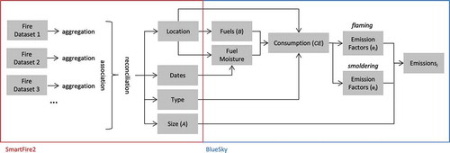
The processing stream used for the CFIRE inventory work is shown in Figure 2. Processing of the emissions inventory requires (a) combining fire information, (b) obtaining vegetation and fuel loading data for each fire, (c) obtaining fuel moisture pertinent for each fire, and (d) modeling consumption and emissions. The methods for each step are described below, along with comments on the inherent uncertainties involved in this type of work drawn from both previous studies (e.g. Larkin et al. 2012) and extensive discussions with scientists and managers undertaken by the U.S. National Wildfire Coordinating Group’s Smoke Committee and the U.S. EPA Office of Air Quality Planning and Standards. These discussions began after the 2008 inventory process, and they helped motivate and guide the work described here through ongoing discussions that occurred throughout the 2011 and 2014 inventory development processes.

Figure 2. Data flow used to process fire information through to calculated emissions. Specific processes and models used in the processing steps are discussed in Sections 2 and 3. Steps corresponding to parts of Equation (1)(1) $\mathrm{E}\mathrm{m}\mathrm{i}\mathrm{s}\mathrm{s}\mathrm{i}\mathrm{o}{\mathrm{n}}_i=A\times B\times \mathrm{C}\mathrm{E}\times e_i$(1) are indicated

Past work has shown that the completeness and accuracy of the fire activity information used is extremely important for the final emissions inventory (e.g. Larkin, Raffuse, and Strand 2014). This was the motivation for the extraordinary effort to collect all available fire information for the 2011 and 2014 National Emissions Inventories. Additional modifications were made to the 2014 inventory development processes based on lessons learned from the 2011 effort.

Modeling systems and software

Two main modeling frameworks were utilized in this work (Figure 2). The SmartFire version 2 (SmartFire2, SF2) fire information system (Raffuse et al. 2012) was utilized in the aggregation, association, and reconciliation processing of all of the fire information datasets. The SF2 processing is explained in Section 3. The BlueSky Framework version 3.5 (Larkin et al. 2009) was used to process the fire information, after it was reconciled into a coherent single dataset, through to speciated emissions.

SmartFire 2 fire information system

SF2 is a modular, open framework developed in Java that facilitates the collection, processing, and reconciliation of an indefinite number of fire information datasets (e.g. ground reports, satellite-based detections, helicopter perimeters). SF2 is not itself an algorithm, but a processing framework. SF2 contains separate functions for ingestion and processing of data from an individual source, association of fire information across different sources over space and time, and reconciliation of different information from different sources to form a single, unified dataset for further processing (in this case, emissions calculations). See Section 3 for further details including the reconciliation capabilities of SF2, as well as Supplemental Appendix C.3 for access to the SF2 codebase.

BlueSky Framework version 3.5

The BlueSky Framework version 3.5 is a modular, open source framework that links various models and datasets to allow for the calculation of emissions and smoke dispersion based on basic fire information and weather model inputs. BlueSky is primarily written in Python but uses the native languages for various incorporated models. Each native model is placed in a python wrapper that allows it to be linked at a sequence of prescribed processing steps, specifically: (1) fire information, (2) fuel loadings, (3) total consumption, (4) time rate of consumption, (5) speciated emissions, (6) plume rise, and (7) smoke dispersion. For the processing used here, fire information from SF2 was provided to BlueSky, which was then run through all the steps up through the speciated emissions modeling step (step 5 above). BlueSky allows the user to select which model/dataset to use in each processing step. Where additional information was available by the reporting system, this information was used preferentially in the emissions calculations for the CFIRE inventory.

Fire activity data

Fire activity data represents the amount of area burned, the location and timing of the fire, and the type of fire (wildfire vs. prescribed burn). The development of a coherent merged fire activity dataset was a major effort in the processing of both the 2011 and 2014 inventories (discussed in Section 3). Raw input fire activity datasets were first gathered from satellite data providing fire detections and national datasets of observations of fires used by the wildfire and prescribed fire communities. Additionally, regional data were assembled from state, local, and tribal (SLT) agencies. At a minimum, input datasets were required to include information about the date, location, and size of individual fires. Ground report data from SLT and national sources were also required to provide information on fire type (wildfire or prescribed burn).

Satellite fire data

Satellite fire information was utilized as processed through the National Oceanic and Atmospheric Administration’s (NOAA’s) Hazard Mapping System (HMS) (McNamara et al. 2004; Ruminski et al. 2006). HMS is an operational effort to collect, assess, and provide human quality control to fire detection data integrating a variety of satellite-based remote sensors. For 2011 and 2014, HMS included automated detections from two types of instruments: geostationary (Geostationary Operational Environmental Satellite (GOES); Schmidt and Prins 2003) and polar-orbiting (Moderate Resolution Imaging Spectroradiometer (MODIS); Giglio et al. 2009, and Advanced Very-High Resolution Radiometer (AVHRR); Flasse and Ceccato 1996). HMS also includes fires detected by trained analysts, who observe smoke plumes in visible satellite imagery and remove likely false detects (such as at gas flares). HMS fire information includes a timestamp and location of the fire detection. Typically, any large fire will include a number of specific fire detections on different days and in different locations. For fires where only HMS data were used, fire size and type assignments needed to be made to process the emissions; this assignment is discussed in Section 3.

Agricultural burning is not included in this inventory. To exclude presumed agricultural burns, the USGS 30-m land use/land cover map was used and HMS detections in “cultivated crops” and “pasture hay” land cover classifications were removed. Note that rangeland fires are included in the inventory.

Although the HMS data includes many fires, the likelihood of detecting a specific fire depends on many parameters, including size, intensity, land cover type, location, timing, and cloud cover. Satellite fire detection is generally worse for smaller fires, fires in lighter fuels, and understory burns; for these reasons, satellite fire detections are better at detecting large wildfires than prescribed fires.

National fire activity databases

National databases maintained by the wildfire and prescribed fire communities were collected. For wildfires, the Incident Command System (ICS)-209 reports and Geospatial Multi-Agency Coordination (GeoMAC) perimeters were utilized; these databases also included some prescribed fires. Information on prescribed fires on the federal Department of Interior and US Forest Service lands was also obtained from the respective agency databases. The National Association of State Foresters (NASF) compiles information on wildfires on state lands; these data were also obtained and utilized.

ICS-209 reports (https://fam.nwcg.gov/fam-web/) are used to report all large wildfires on federal lands as well as some smaller incidents, including some prescribed fires. Other lands owned by states and/or federal cooperators sometimes also report via the ICS-209 reports (NIFC 2017). All fire types are represented in the ICS-209 database, but the majority are wildfires. ICS-209 reports typically include information on fire size, initial ignition or detection latitude and longitude, dates, and type of fire. Notably, ICS-209 reports are manually generated during incident response, which can sometimes result in errors.

GeoMAC perimeters (http://rmgsc.cr.usgs.gov/outgoing/GeoMAC/) are usually produced by geographical information system (GIS) specialists working on wildfire incidents. GeoMAC information generally includes a final fire perimeter along with limited metadata, including dates and type of fire. In some cases, periodic perimeters showing the progression of the fire are also available. GeoMac perimeters are not always available, even for a large wildfire, and the final perimeter sometimes includes portions of the overall fire perimeter that did not actually burn; this inclusion of unburned interior islands within the fire or other land not affected can exaggerate the GeoMac area burned. Intermediate progression perimeters are subject to revision and refinement on different days and may show negative growth between sequential perimeters. Since these emissions inventories are retrospective, the final available perimeter is used, but if negative growth occurs it is set to zero. Some perimeters may also include topology errors that must be corrected before processing.

Federal land management agencies, specifically, the U.S. Department of Agriculture Forest Service (USDA-FS) and the U.S. Department of Interior (DOI), supplied their internal databases of prescribed fires. The USDA-FS uses the Forest Service Activity Tracking System (FACTS, https://data.fs.usda.gov/geodata/edw/datasets.php). The DOI uses a database called the National Fire Plan Operations and Reporting System (NFPORS; https://www.nfpors.gov). The U.S. Fish and Wildlife Service (USFWS), part of the DOI, also tracked prescribed fires separately and provided its own database. The FACTS, NFPORS, and USFWS data were extracted by the agencies at the request of USDA-FS personnel who were involved in shaping the 2011 and 2014 efforts described here. FACTS and USFWS data were incorporated in both the 2011 and 2014 inventories, and NFPORS data were incorporated in only the 2014 inventory. The FACTS, NFPORS, and USFWS datasets contained only prescribed burn information, and the size, location, and date of the burn were available for each fire. For 2014, some perimeters were also available (use of perimeters has increased in subsequent reporting years). Both the FACTS and NFPORS databases suffer from differential adoption. Depending on the specific site managing the burn, more or less information might be input into the database, and the specific type of information provided might vary, such as reporting planned versus accomplished acreage. We use accomplished acreage where it is provided, but fall back to planned acreage if it is not.

Wildfires on state jurisdiction are compiled by the NASF. The NASF data (https://fam.nwcg.gov/fam-web/) include many small fires occurring on state-owned land that are not available in federal datasets. NASF data includes records of wildfires collected by the association via the NASF Fire Reporting website. The specific coverage, in terms of fire size, type, land ownership, etc., of the NASF data varies from state to state depending on the original fire reporting data sources.

Regional fire activity databases

In addition to satellite-derived fire information and national fire activity databases that were available for all areas, a concerted effort was made by the EPA to obtain regional – including state, local, and tribal – fire activity databases. For 2011, 50 databases containing data in 20 states were obtained. For 2014, 55 databases containing data in 22 states and one tribal nation were obtained. A complete list of datasets is given in the available supplementary materials accompanying this paper (Supplemental Appendix A, Table A.1). Some datasets had to be excluded (19 in 2011, 22 in 2014) because they did not have the minimum data (size, location, dates) required to process the data through emissions. Figure 1 shows where regional, state, local, and tribal data were utilized.

The largest regional database obtained was the Fire Emissions Tracking System (FETS, http://wrapfets.org), operated by the Western Regional Air Partnership (WRAP, 2007) states. Overall data from 10 states in 2011 and 8 states in 2014 were provided through arrangement with the WRAP. The FETS system is primarily designed for prescribed burn reporting, and FETS provides for location, dates, and the capability of listing both planned and accomplished size. Where available, accomplished size was preferred.

After data quality assurance and cleaning, fire activity data submitted by 24 states were used in the development of the 2011 inventory, and data from 22 states and one tribal nation were included in the 2014 inventory.

For 2011, two additional specific adjustments were made through interaction with state and federal agencies. For large wildfires that occurred in Minnesota in an area of deep peat, observed burn depths were provided by local U.S. Forest Service personnel. In the Flint Hills of Kansas, where widespread rangeland burning is common in spring, an estimate of the total area burned for the region was provided by the state using the methods of Mohler and Goodin (2012) and individual fires were scaled to match the provided total.

During 2014 inventory development, in addition to collecting the regional/local fire activity databases, a questionnaire covering metadata useful in interpreting the database was also distributed (available in the accompanying supplementary materials, Supplemental Appendix A, Figure A.1). The questions are designed to allow the submitting agency to declare the expected coverage and completeness included in the dataset in terms of the types of fires, sizes of fires, and land ownerships. For example, if a dataset does not report fires smaller than 100 acres, or does not report fires on military bases, this information could be declared in the questionnaire. This questionnaire was returned by 20 states and one tribal nation (Figure 1, diagonal stripes). Although this questionnaire was voluntary and self-reported, it provided a starting point for assessing the data and understanding whether to prioritize the dataset over the national databases.

For 2014, the specific collection of datasets used in a given state was based on these questionnaires. In five states where relatively complete data were submitted by the state, either no national datasets or only a subset of the available national datasets were used to supplement the submitted data. The South Carolina datasets were reported as 100% complete for all categories; as a result, the datasets were not supplemented with any national datasets. Similarly, Alaska reported 100% completeness for its dataset. However, because each raw data record represented a single wildfire over its entire spatial and temporal extent, the data for Alaska were supplemented with the HMS dataset to provide improved daily fire growth and location information. Any resulting fires that were solely based on HMS data were removed in subsequent processing. The Georgia questionnaire reported that fires associated with a federal primary agency were not included, so only federal data (USFWS, FACTS, NFPORS, and federally reported GeoMAC records) were used to supplement the state’s data. On the basis of Florida’s questionnaire response, its dataset was supplemented with federally reported wildfires only in the USFWS and GeoMAC datasets. At the state’s request, the North Carolina dataset was supplemented with only the FACTS data and USFWS data for Pee Dee and Great Dismal Swamp National Wildlife Refuges.

Pile burns

One methodology used for planned fuel reduction burns is to collect excess fuels into large piles and then burn the piles. This type of prescribed fire is used differentially across the U.S. A known issue of CFIRE, and most other large-scale fire inventories, is that pile burning information was not included in the fire information and subsequent emissions calculations. In several cases, this was because not all of the information needed to compute emissions from piles was included in the databases collected. In these cases, the number of piles was generally available, but the dimensionality of the piles – needed to compute their volume – was not. This issue was part of the reason that Washington State, where pile burns are a substantial component of overall prescribed burn activity, decided to compute their own emissions estimates for inclusion in the NEI.

Databases and models used in emissions calculations

Emissions were processed using the BlueSky Smoke Modeling Framework v3.5. The specific models and databases used in this processing are listed in Table 1; explanations are presented in each processing step subsection below.

Table 1. Models used in the emissions calculations for 2011 and 2014. See Section 2.4 for discussion, and explanation of model names

Process Step	Model
Fuel Loading Maps	FCCS v2
Fuel Moisture Information	WIMS v1
Consumption Model	Consume v4.1
Emissions Model	FEPS v2
Post Processing	Duff Adjustment

Fuel loading maps

Fuel loadings were derived from a map generated for the Fuel Characteristic Classification System (FCCS, McKenzie et al. 2007) version 2 (available at http://www.fs.fed.us/pnw/fera/fccs/maps.shtml). Within FCCS, a list of more than 250 fuelbeds have been created that describe the vegetation of that location from the deep organic soils up through to the canopy. Deep organic soils are of particular importance, where they occur because they can contain large amounts of potentially consumable biomass per unit area. The particular vegetation landscape is given a quantified, detailed list of physical characteristics that drive fire effects (e.g. amount of downed dead wood of various diameters, height of tree canopy, and depth of ground fuels). FCCS fuelbeds have been derived from observations at a number of locations across the country; they have then been mapped by relating the fuelbeds to the LANDFIRE fuels maps to create a 30-m resolution map across the contiguous U.S. and Alaska (Rollins 2009). The 1-km spatial resolution used here was developed from an upscaling of a 30-m resolution map created via a rule-based classification approach. For any fire located in an area that has no fuels on the FCCS map, a substitute fuelbed from a nearby area with low fuel loading was assumed.

Fuelbeds vary considerably based on the plot data used and the spatial mapping algorithm applied (e.g. Larkin, Raffuse, and Strand 2014). The techniques used are unlikely to capture the actual variability of fuel loadings at specific locations. Independent plot measurements have shown little overall bias in the FCCS mappings, however (Larkin et al. 2012).

Fuel moisture information

The amount of fuel consumed, as well as the ratio of flaming to smoldering combustion, is governed in part by the moisture conditions of the fuel at the time of the burn; for this reason, fuel moisture is an input to the fuel consumption step. Daily fuel moisture values were acquired from the Weather Information Management System (WIMS, http://www.wfas.net/archive/www.fs.fed.us/land/wfas/archive/). Daily temperature, humidity, and rainfall observed at Remote Automated Weather Stations (RAWS) across the United States are used to compute fuel moisture for dead fuels of varying diameters as classified by the National Fire Danger Rating System (NFDRS) (Deeming 1972). Each fire was assigned the fuel moisture values for the nearest reporting RAWS. If no station within 300 km was found, fire type-specific (wildfire or prescribed burn) default values were used.

Fuel moisture assignments may differ from the actual fuel moistures observed on a fire due to the limited spatial sampling of the network of monitors used to map fuel moistures along with the highly localized spatial scales associated with precipitation.

Consumption model

CONSUME model version 4.1 was used to estimate consumption (Ottmar 2014; Prichard, Ottmar, and Anderson 2006; Prichard et al. 2017). This step in Equation (1)(1) $\mathrm{E}\mathrm{m}\mathrm{i}\mathrm{s}\mathrm{s}\mathrm{i}\mathrm{o}{\mathrm{n}}_i=A\times B\times \mathrm{C}\mathrm{E}\times e_i$(1) focuses on the determination of the consumption efficiency (CE). While consumption efficiency can be computed from CONSUME outputs, CONSUME itself uses fuel moistures and fuels information stratified by fuel category – such as duff, litter, canopy, and downed woody debris in size classes from FCCS fuelbeds – along with other factors to calculate the fire energetics in order to determine consumption by combustion phase, specifically: flaming, smoldering, and long term smoldering (also known as the residual phase). By differentiating combustion phases, specific emissions factors can then be applied to the flaming and smoldering (both smoldering and long-term smoldering) phases in the emissions factors step (Section 2.4.4). These emissions factors reflect the fact that combustion phases have different consumption efficiencies and therefore speciate emissions differently.

CONSUME’s consumption calculations have been fit empirically to pre- and post-burn data from more than 100 sites across multiple forest and shrubland ecosystems. This includes different fits for different regions of the country. The specific fit to use for a given fire is determined by the fire’s location. (Note: Based on comments from the State of Minnesota and in consultation with the model developers, the “boreal” region consumption equations were used in place of the “western” region equations for Michigan, Minnesota, and Wisconsin. The boreal equations have refined duff consumption equations from empirical studies (Prichard, Ottmar, and Anderson 2006) that were determined to be more representative for this region.) Additionally, CONSUME contains settings for wildfire versus prescribed fire; for prescribed fires, for example, canopy consumption is limited.

Emissions factors

Separate emission factors for flaming and smoldering consumption for nine species (CO2, CO, PM2.5, PM10, NOx, SO2, NH3, and total VOCs) were applied through the Fire Emissions Production Simulator (FEPS) as implemented in BlueSky. The overall effective emission factors depend on the modeled ratio of flaming to smoldering, which is determined by the consumption modeling step (Section 2.4.3). The emission factors from FEPS for flaming and smoldering are provided in the Supplemental Appendix C, Table C.3.

Post processing

Duff consumption for prescribed fires was adjusted as a post-processing step because of a known issue in the CONSUME 4.1 model, where unrealistically large duff consumption can occur in areas of large duff depths. Because this issue was flagged by regional experts working with the National Wildfire Coordinating Group (NWCG) Smoke Committee, a post-processing limitation was imposed on prescribed fire duff consumption of 44.8 tonnes/ha (20 tons/acre) in the western United States (all states west of Texas, plus the Dakotas) and 11.2 tonnes/ha (5 tons/acre) in the eastern United States. No limitations were placed on wildfire duff consumption except in the case where explicit duff depth information was provided from local experts (2011 Minnesota).

Development of a combined fire information reconciled dataset

Development of the 2011 and 2014 emissions inventories was designed to identify and include fire information from as many fire activity data sources as possible. This approach differs from previous efforts in two ways: (1) it was designed to combine all available data sources and to rely on a single source as little as possible; (2) it was specifically designed to produce a temporally explicit fire growth history due to the need to use these data to create a time-resolved emissions inventory. By combining all available data sources, this inventory is in a different category than single-source inventories such as those created from satellite data (Global Fire Assimilation System (GFAS), Kaiser et al. 2012; Global Fire Emissions Database (GFED), Van der Werf et al. 2010; Fire INventory from NCAR (FINN), Wiedinmyer et al. 2011). Combining data sources necessarily accepts less uniformity in the available data in order to create a more inclusive, and hopefully more complete, dataset. Creating a temporally explicit (daily growth) inventory differentiates this effort from other comprehensive assessments of wildland fire activity like the Fire Program Analysis fire occurrence database (FPA FOD; Short 2015), where only the overall period (start date and end date) of the fire is recorded.

A major focus of this effort was to combine fire information into a reconciled dataset that could then have emissions calculated without double (or further) counting the same fire. To combine data, the SmartFire 2 fire information system (SF2) was utilized. The process described here is the fundamental process built into the SF2 system; this section can be considered a description of SF2, albeit with specific application to the datasets developed for 2011 and 2014.

Within SF2, there are three steps: (1) aggregation and expansion of the data within each source dataset; (2) association of data across datasets; and (3) reconciliation to create a unified dataset.

Aggregation and expansion of the data within each source dataset

Each individual data source was processed to accomplish two goals: (1) to aggregate the data into a single consistent fire entity, and (2) to process the data such that all of the fire information fields needed are filled in.

Aggregating the data into a single fire entity primarily affects satellite data. Satellite fire detections differ from other data sources in that a single “fire” may be represented by many satellite detections across many days. Satellite data were aggregated by creating buffer regions and tracking detection points across days to produce daily burning areas, including daily fractional growth and an overall final fire shape (see the accompanying supplementary materials, Supplemental Appendix B). Aggregating multiple data points into a single fire entity is also required for some other data sources, but the aggregation is typically trivial (e.g. linking reports from multiple dates with the same fire ID).

The following fields are created for each fire represented by a data source:

• Location (latitude, longitude)*

• Final size* and/or shape

• Start date*

• End date

• Daily fractional growth

• Name (where available, otherwise assigned a unique identifier)

• Fire type (e.g. wildfire or prescribed burn)

*Fire location, size, and start date are considered the minimum required input information from any dataset, except for satellite fire detections, where an area assignment was utilized to fill in fire size.

Fire information quality assurance and cleaning

Fire activity datasets were quality-checked before inclusion. The first check was to ensure that the minimum necessary information was included. Datasets were further cleaned, and dataset formats were standardized. Typical cleaning steps included correcting or removing fire locations outside the United States, correcting poorly formatted dates, and correcting end dates that fell either before the start date or at implausibly later than the start date.

Assignment of fire size to satellite fire detections

The satellite-detected active fire products (thermal anomalies) used in this work do not directly observe fire size. To process such data through emissions in the absence of another source that contains fire size, the detections must be assigned a fire size. However, the energy of a fire detected by the satellite varies according to multiple factors, including the intensity of the fire at the time of observation, the amount of cloud cover, and the observation angle. These factors affect the ability of the satellite both to correctly identify a fire and to assign an underlying fire size to a satellite detection. To assign per pixel fire size, the results of an analysis relating the ratio of final fire size from the Monitoring Trends in Burn Severity Project (Eidenshink et al. 2007) ground observations to the number of satellite fire detections observed during the course of the fire was used (Raffuse et al. 2012). This analysis developed a linear fit based on vegetation classes produced from the 1-km FCCS map. The result is a per-satellite fire detection default area assignment that varies from class to class, with a minimum size of 18.6 ha (46 acres) per detection in closed-conifer regions to a maximum size of 81 ha (200 acres) per detection in shrublands. All of the per-detect area estimates are lower than those used in FINN, which also estimates area from (MODIS only) active fire detects (Wiedinmyer 2011).

Assigning fire size in this manner will reproduce the overall statistical fit to the final area burned across multiple fires. However, for individual fires, the default size assignments may be too high or too low to properly add up to the actual final fire size. Assigning fire growth in this manner necessarily incorporates the issues with satellite observations (e.g. cloud cover, overpass time, viewing angle) into the daily progression. For this reason, satellite fire size estimates are assigned a low rank in the reconciliation process and are therefore only used as a last resort. The resulting day-to-day variations in detection rates will produce artificial variations in daily area burned.

Assignment of fire type where unknown

The type of fire – wildfire or prescribed fire – affects consumption assumptions, specifically canopy involvement, which subsequently influences calculated emissions. Assignment of emissions to either wildfire or prescribed fire is also important for emission inventory users. To assign a fire type when the fire type is otherwise unknown, in the case of HMS fire detections, a climatology based on an analysis of historical patterns of wildfires versus prescribed fires was utilized. The climatology (shown in Table 2) identifies a set of calendar months when wildfires are more likely by state, and fires that start in this period are assumed to be wildfires in the absence of specific fire type information. Conversely, fires that start beyond this period are assumed to be prescribed fires.

Table 2. Climatology used for assignment of fire type when no other information on fire type is available by state. Periods show when a fire is assigned by default to be a wildfire; outside of these periods the fire is by default assumed to be a prescribed burn. See Section 3.1.3 for discussion

States	Months Assumed Wildfire
Alaska	May–August
Washington, Oregon, Idaho, Montana, Wyoming, Colorado	June–August
California, Nevada, Utah	May–October
Arizona, New Mexico	April–July
All Others	None

This assignment has known issues, and other methodologies are in development and have been used since the emissions inventories described here. The historical calendar year assignment can be off base on the evolution of the particular year, which may have a wildfire season that starts earlier or last later than the period identified by the climatology. To better define the prescribed fire periods for that particular year, a recommendation of this work is to do a year-specific calendar, or to look at known prescribed fire windows compared with observed weather.

Association across data sources

To identify where two or more data sources were representing the same fire, the overall spatial extent of the fire along with the time period of the fire was used to create a four-dimensional spatio-temporal shape. Overlaps between shapes from multiple data sources were then identified and recorded. In this process, no judgment of which representation better describes the fire is made, and no attempt at reconciling different information is done; only associations between the data coming from the different sources are made. To properly identify overlaps between the data sources, the spatio-temporal overlap is identified taking the uncertainty of each data source into account. Each data source is assigned uncertainty for start date, end date, and location, which is added to the “footprint” of each fire. Any fire from different data sources that occurs within overlapping footprints is associated.

Reconciliation of data sources into a combined fire information dataset

If more than one data source identifies a fire (i.e. fires originating from two or more datasets are associated), the information must be reconciled in SF2 to produce a single dataset that avoids double (or more) counting of the fire. Instead of selecting all the information from a single data source, each fire information field listed above is treated separately, taking into account the strengths and weaknesses of each dataset. Figure 3 provides an example of this process.

Figure 3. The SF2 fire data reconciliation process demonstrated for a large wildfire from the CFIRE emissions inventory. Here, fire data from satellite fire detections (left/red, i.e. HMS data), aerial surveys or GPS perimeters (center/orange, i.e. GeoMAC perimeters), and ground reports (right/blue, i.e. ICS-209) are merged, preserving the most accurate available information for fire size (from aerial surveys), type (from ground reports), start date (from satellite detections), and end date (from satellite detections)

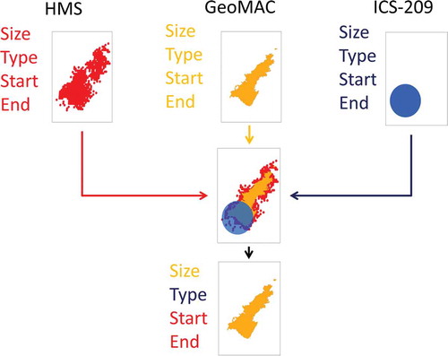
In performing this assignment, an assessment of the relative strengths of each data source for each fire information field is utilized to create a separate precedence for which data source to use for each fire information field. For example, fire perimeter data from aircraft overflights may provide an accurate estimate of the location and shape of a burn, but they do not provide useful information about the end date of the fire. Therefore, aircraft overflight perimeters are highly ranked for shape information, allowing them to be preferentially used for this information, but are assigned a low ranking for end date information, so that they are used for this purpose only if no other data set is associated with the fire.

The specific preferences used for fire information reconciliation in the 2011 and 2014 CFIRE inventory calculations are shown in Table 3. The following generalized rules were applied:

• Polygon datasets, including GeoMAC, some regional data for 2011, and FACTS for 2014, were given the highest preference for fire location, shape, and size. For fire location and shape, HMS data were given the next preference because of the likelihood of multiple observations by multiple satellites for a given fire event detected. Point-based data sets were used last.

• HMS data received the highest fire growth preference due to the likelihood of multiple observations per day from multiple satellites for a given fire event detected. Data sources where multiple observations were possible on different days for a given event, including GeoMAC, ICS-209, and some regional data for 2011, were used next.

• ICS-209 and GeoMAC data received the highest preferences for fire name and fire type because they are the primary and often the most comprehensive national data sources for large fire events.

• Regional datasets, including state, local, NASF, and FETS data were used next whenever possible after the above rules were applied, followed by federal data sources (i.e. ICS-209, FACTS, NFPORS, and USFWS).

• HMS data received the lowest preference rating for fire size, name, and type because size and type had to be inferred, and name was unknown for satellite fire detections.

Table 3. Preference order used in fire data reconciliation for the CFIRE inventories

	Location/Shape	Overall Size	Daily Growth	Fire Name	Fire Type
1	National DB Polygon	Regional DB Polygon	Daily Satellite Detections	National DBs (WF)	National DBs (WF)
2	Regional DB Polygon	National DB Size (WF)	National DB Size/Polygon (WF)	Regional DBs	Regional DBs
3	Satellite Polygon	National DB Polygon	Regional DBs	Satellite Unique ID assigned	Climatology
4	Regional/National DB Points	Regional DB Size (WF)
5	National DB Points	Regional/National DB Size (RX)
6		Satellite Assigned Size

Some specific preferences differed between 2011 and 2014 because of data availability and our knowledge of the datasets at the time of data evaluation. Not all the reasons for the differences are discussed here, but noteworthy ones include:

• FACTS data were point-based for 2011 and polygon-based for 2014.

• Regional data for 2011 varied in dimensions both spatially (some point-based and some polygon-based data) and temporally (some contained multiple daily records per fire while some contained only one record per fire).

• NASF data for 2011 were supplied late in the process. With limited knowledge and time to evaluate, low preferences were assigned to it for fire location, shape, size, and growth.

See the accompanying supplementary materials (Supplemental Appendix A, Table A.1) for a complete list of fire data sources.

Results for 2011 and 2014

The CFIRE emissions inventories for 2011 and 2014 are located at https://ei.airfire.org/data/cfire along with supporting documentation. The inventories are in comma-separated-value files formatted into a data model that provides not only hourly emissions data at specific locations but also summary data for specific fire events. The inventory files, data model, and supporting documentation are further described in the supplementary materials (Supplemental Appendix C).

Annual totals

Table 4 shows a summary of overall totals for the 2011 and 2014 CFIRE inventories. Averaging between 2011 and 2014, fires burned 7.75 Mha. Of these, prescribed fires accounted for 50.5% of the number of daily fires but 61.1% of the total area. This difference between prescribed burn size versus percentage in fire counts reflects the large number of very small wildfires (<0.5 ha) included because a majority of the wildfires included either did not grow appreciably or were quickly suppressed. Average emissions across the two inventories were approximately 242 M tons of CO2 and 1.74 M tons of PM2.5. Of this, prescribed fire accounted for 48.5% of CO2 but only 44.5% of PM2.5. This is because the largest wildfires in the inventory for those years had above-average PM2.5-to-CO2 emissions ratios. High PM2.5 emissions rates and PM2.5-to-CO2 emissions ratios were associated with heavy duff consumption in these wildfires.

Table 4. 2011 and 2014 CFIRE inventory totals for the contiguous U.S. and Alaska, including number of fires, total area (in 10⁶ hectares and also shown in 10⁶ acres), and emissions (in 10⁶ metric tons). Results are shown for all fires and are also split out for wildfires and prescribed (Rx) burns. Fire counts are the number of fire days within the inventory, where each fire is counted once per burning day of its duration

		2011 CFIRE			2014 CFIRE
		Wildfire	Rx Burns	All	Wildfire	Rx Burns	All
Fire counts		121,128	104,812	225,940	80,185	100,163	180,348
Total area in 10^6 Ha (in 10^6 acres)		4.32(10.68)	5.03(12.43)	9.35(23.11)	1.72(4.24)	4.43(10.94)	6.14(15.18)
Emissions in 10^6 tons	CO2	149.06	125.99	275.05	99.32	108.17	207.49
	CO	13.33	9.51	22.85	9.39	8.01	17.41
	VOC	3.14	2.25	5.39	2.21	1.90	4.11
	PM10	1.34	0.99	2.33	0.94	0.84	1.78
	PM2.5	1.14	0.84	1.98	0.79	0.71	1.50
	CH4	0.65	0.47	1.12	0.46	0.40	0.85
	NH3	0.22	0.16	0.38	0.15	0.13	0.28
	NOx	0.17	0.15	0.32	0.11	0.14	0.24
	SO2	0.10	0.08	0.17	0.06	0.07	0.13

Differences in the overall extent of fire between these two years are evident, with 2011 the larger fire year. 2011 had 25% more fire locations and 52% more fire area burned, driven mostly by more wildfires (+51%) and more overall wildfire area burned (+151%). The result was 33% more CO2 emissions than in 2014, and wildfires accounted for 50% of this total; PM2.5 follows a similar pattern. In contrast to the difference in wildfires between the two years, the results for prescribed fires are quite similar. Overall, while prescribed fires contributed significantly in all aspects to the overall emissions inventory, wildfires drove the major differences in total emissions between the two inventories.

CFIRE’s 2011 and 2014 total PM2.5 emissions average represents 32% of the all-sector total U.S. PM2.5 emissions, as estimated in the respective NEIs, including all stationary, mobile, and non-wildland fire natural sources. The total for wildland fire emissions is five times larger than all U.S. mobile sources combined, including passenger vehicles, trucks, construction equipment, trains, and aircraft. This estimate is also roughly equivalent to estimates of total man-made PM2.5 emissions for Europe (1.55 M tons in 2014; OECD, 2019). However, it represents only about 5% of the average annual global PM2.5 from open biomass burning estimated by global models (Van der Werf et al. 2017).

Table 4 also shows the daily fire counts for 2011 and 2014, with the two years showing an average of 203,144 daily fires per year. Here daily fire counts are defined as the number of fire days, where each fire is counted once per burning day within its duration. This helps account for fires of widely different durations, and more closely represents the number of unique fire emissions sources within the inventory. Note that the number of fires is one of the quantities that varies the most between biomass burning inventories, including those analyzed here, because it depends critically on methodology; some grid-based inventories aggregate all burning activity within a grid cell, or alternatively split out large fire events into multiple fire detections. Where possible, CFIRE tries to alleviate these issues, using ground-based fire reports to keep distinct fires separated, and using grouping and tracking of satellite detections of fires across days (see the accompanying supplementary materials, Supplemental Appendix B) to keep extended burning areas associated as a single fire. This makes the CFIRE fire counts more similar to the human-understandable concept of a fire. While this number is not directly comparable to other emissions inventories, it does provide a fundamental sense of the number of fire emissions sources throughout the year.

Results by state and spatial patterns

Examining the results by state shows the spatial patterns of fire within each year. Figure 4 presents the area and CO2 equivalent (CO2e, here computed as CO2e = CO2 + CH4*25) totals by state for each inventory. The overall prevalence of prescribed fires in the Southeast is seen in the top panels, with the bulk of each state’s burned area due to prescribed fires. Wildfires account for a greater percentage of each state’s area in the western U.S. and Alaska. Major differences in the amount and location of wildfires across the West are evident, with large wildfires occurring in Texas, New Mexico, and Arizona in 2011, and significant fires occurring in Washington, Oregon, and California in 2014. Differences in wildfires in the Southeast, such as the wildfires in Georgia in 2011, can also be seen, but these cause a smaller proportional change in state emissions because of the large amount of prescribed fires that remains relatively consistent across both years.

Figure 4. State totals of area burned and CO2 equivalent (CO2e) emitted for the 2011 and 2014 CFIRE inventory. Wildfire totals shown in red; prescribed burn totals shown in green. Pie sizes are proportional to state totals

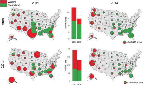
Notably, the amount and location of emissions in 2011 appear disproportionate to the area burned within Minnesota and North Carolina. This is due to the deep organic consumption in fires in these areas. Deep organic consumption has been observed to produce considerable amounts of emissions in various fires (Page et al. 2002). However, calculating the exact amount of consumption is a known issue (Larkin et al. 2012; Ottmar 2014) within the consumption models themselves, and it also required specific attention in the modeling done for the CFIRE inventory (Section 2.4.5). For 2014, the deep organic consumption calculation was less of a factor simply based on the location of the fires that occurred.

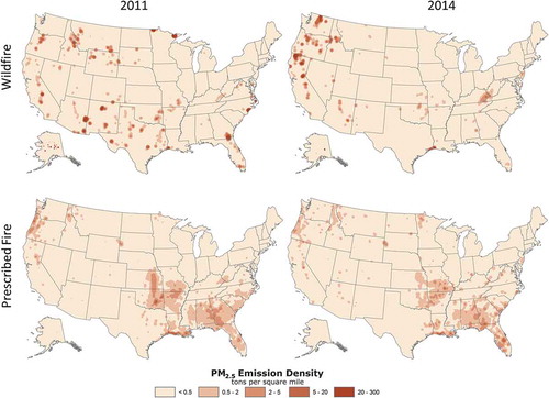
Consumption and emissions for specific fires can have a significant impact on state and national totals, which can be seen by plotting emissions density (Figure 5). This is particularly true for wildfires, where the intensity of the burn can raise the overall amount of consumption per unit area, creating emissions hotspots that vary considerably by year. By contrast, the large number of prescribed fires distributed across the Southeast occurred at lower intensity and therefore showed, in aggregate, more consistency across years.

Figure 5. Annual wildland fire PM_2.5 emission totals shown as tons emitted per square mile for each location. Both the 2011 and 2014 CFIRE inventory are shown and are separated into wildfire and prescribed burn annual totals

Seasonal cycle

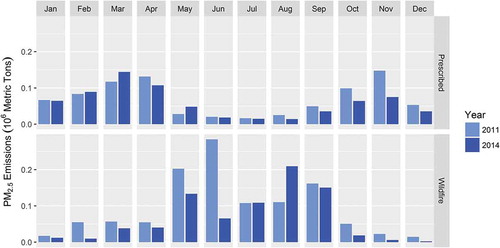
The relative consistency of prescribed fire emissions versus wildfire emissions can also be seen in the seasonal pattern of emissions (Figure 6). For prescribed fires, there is an overall pattern of spring and fall emissions, with more limited emissions in the summer and winter. The 2014 prescribed burn emissions show a slightly higher spring emissions season, but a much lower fall emissions season. However, the overall pattern is more consistent than for wildfire emissions, which jumped from month to month based on the specific wildfires that occurred. For wildfires, 2011’s summer had more early (May/June) emissions than 2014’s, and generally had more or similar emissions for every month except August. For both years, wildfire emissions were greater in May through September, while prescribed fire emissions were greater in October through April.

Figure 6. PM2.5 emissions by month for the CFIRE inventory. Split out by year (2011 and 2014) and by wildfire vs. prescribed fire

Discussion

The results provided here take advantage of a variety of fire activity data sets derived from satellite detections, operational ground reports, and state and local prescribed-fire permitting programs. These various fire information systems have their strengths and weaknesses, and combining them into a reconciled and unified fire emissions inventory presents unique challenges. The strengths and weaknesses of each dataset must be taken into account in how they are combined with other datasets. Some databases have de minimus sizes below which fires are not included. Others include fires only on certain land ownerships. Wildfire reporting is different depending on the overall level of fire suppression response invoked; major wildfires typically report much more information than small wildfires. Many national prescribed fire reporting systems are differentially utilized by different agencies or parts of the agency; for example, some national forests may provide more complete or accurate data than others. State databases can also sometimes include data from neighboring states where specific land management agreements exist. Deciphering these differences requires the expertise of those most familiar with the specific nature of the workflow that allows data to become part of the database.

A large-scale effort was needed to collect, understand, and merge these data for the 2011 inventory. Each database was analyzed and then discussed with local experts before inclusion to understand what was needed from a quality assurance perspective, to understand the overall reliability of the data for dataset prioritization and quality assurance, how the dataset fit with other data covering the same spatial area. Lessons learned from this effort led to an initial questionnaire that was incorporated into data request for the 2014 inventory. The result of this effort was to develop a preference order for which datasets to rely on within various polygons based on state boundaries or land ownership, differentially stratified for prescribed fires and wildfires.

Influence of data sources

A major question for this work is how the inclusion of additional datasets affected the overall results. One measure of this is to examine the fire area burned and emissions found in each of the source datasets. Table 5 shows the percentage of overall daily fires, area burned, CO2, and PM2.5 emissions found in the national, satellite, and regional databases, including overlaps between the three kinds of datasets. The area burned and PM2.5 breakdowns are also shown as Euler diagrams in Figure 7. Satellites alone accounted for the plurality of the fire area, with 38.5% (2011)/34.2% (2014) of the total area represented. Fires found in both satellite and national databases accounted for 27.7% (2011)/20.8% (2014) of the total area. In 2014, more fires used only regional data (27%) than in 2011, based on the states and regions self-reporting these datasets as complete. Where this was determined to be viable, through the 2014 questionnaire and discussion with the state agencies, satellite and national databases were not reconciled together with the state data. This reduced the percentage of fires using data from all three kinds of sources from 18.5% to 3.5% of the total area. Even in 2011, fires reported only in regional datasets accounted for over 5% of the total area burned. This provides a lower limit of the effect of including the regional data. For an upper estimate, overall the regional data were used in fire information representing 28.7% (2011)/36% (2014) of the total area burned. Indeed, even in the 2011 effort, the regional datasets provided information on more fires (44.5%) than did either the satellite (42.7%) or national (44.1%) datasets.

Table 5. Fire information source types contributing to fire area, CO2 emissions and PM2.5 emissions

	2011				2014
Source Types Used	Fire counts (% of Total)	Area (% of Total)	CO2 (% of Total)	PM2.5 (% of Total)	Fire Counts (% of Total)	Area (% of Total)	CO2 (% of Total)	PM2.5 (% of Total)
National only	22.4	5.2	4.9	4.8	29.5	9.1	9.0	8.6
Satellite, National	6.8	27.7	28.8	28.5	4.5	20.8	31.5	34.6
Satellite only	26.3	38.5	32.3	30.5	22.1	34.2	27.3	26.2
Regional, Satellite	3.6	4.4	4.6	4.5	2.0	4.5	10.1	12.1
Regional only	26.0	5.2	4.8	4.5	36.8	27.0	16.6	13.1
Regional, National	8.9	0.6	0.9	0.8	4.2	1.0	1.1	1.0
Regional, Satellite, National	6.0	18.5	23.8	26.5	1.0	3.5	4.5	4.4

Figure 7. Euler diagrams showing fire information data sources that went into the final fire emissions inventory by type of data sources used for each fire. Numbers presented are percentages of total area and percentages of total PM2.5

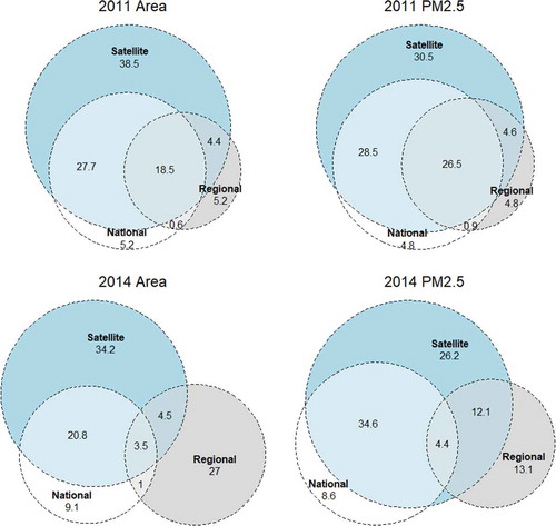
The top three data source combinations for total area in 2011 are (1) satellites alone, (2) satellite plus national databases, and (3) satellite, national, and regional databases. Together, these account for 84.7% of total area burned and 85.5% of total PM2.5 emissions. In 2014, the top three data source combinations are (1) satellites alone, (2) regional databases alone, and (3) satellites plus national databases, accounting for 82% of total area burned and 73.9% of total PM2.5 emissions. Regionally, reported fires make up 27% of the total area burned in the 2014 inventory, yet contribute only 13.1% of the total PM2.5 emissions. This is likely because these fires are predominantly prescribed fires with lower per-acre emissions. Because of the 2014 questionnaire, several state databases were able to be determined to be complete and not in need of reconciliation with satellite and other data. This accounts for the drop in satellite data between 2011 and 2014. This also affected primarily the identification of prescribed fires, as the use of regional databases alone occurred mainly in areas with large prescribed burn activity, specifically Florida, Georgia, Alabama, South Carolina, and North Carolina.

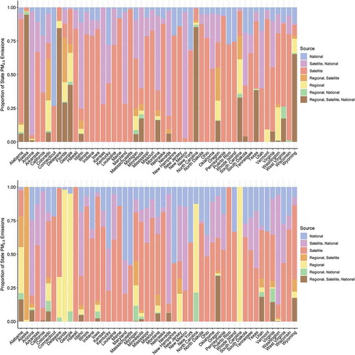
The overall breakdown of data source influences listed above varies considerably state by state (Figure 8) because of several factors: (1) data coverage and completeness voluntarily reported in the fire activity database questionnaire, (2) the relative amounts of prescribed fire activity and wildfire activity within the state, (3) efforts within the state to gather prescribed fire (and sometimes wildfire) information usually as part of a prescribed fire permitting system, and (4) the ability of satellites to detect the type of prescribed fires and wildfires typically found in that state. For example, the prevalence of low-intensity, understory prescribed fires that are difficult to detect by satellite is higher in some states than others.

Figure 8. State by state breakdown of percent of the fires in that state that utilized different types of databases for the (top) 2011 and (bottom) 2014 CFIRE inventory

Comparison with state emissions inventories

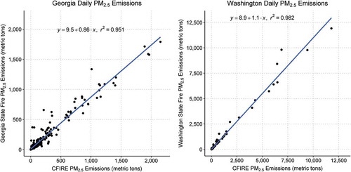
The CFIRE inventory results are hard to validate independently because they represent the only effort to collect and reconcile all of the source datasets used here. However, specific comparisons can be made in areas that have well established and well-regarded fire information systems that track prescribed fires. Additionally, Georgia and North Carolina submitted their own wildland fire emissions calculations for the 2011 NEI, and Georgia and Washington submitted their own calculations for the 2014 NEI. Of these, Georgia and Washington are perhaps the best developed inventories, and they also provide contrasting levels of prescribed fires and wildfires in 2014.

Figure 9 shows the county-by-county 2014 CFIRE inventory compared with the state-developed emissions for each county in Georgia and Washington, including both wildfires and prescribed fires. Overall, the CFIRE inventory closely tracks the two state-developed emissions inventories. This is expected because both Georgia and Washington provided their state fire information to the CFIRE inventory effort. Still, it provides evidence that the association and reconciliation of multiple fire information sources were largely successful at avoiding the double-counting of fires because these fires were also represented in other databases aggregated and reconciled within CFIRE. For Washington, CFIRE PM2.5 emissions are 11.4% (12 x 10³ metric tons) lower than the state-submitted emissions. For Georgia, CFIRE PM2.5 emissions are 8.0% (4 x 10³ metric tons) higher than the state-submitted emissions.

Figure 9. Comparison of 2014 CFIRE PM_2.5 emissions with state-reported emissions

Comparison with other inventories

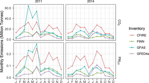
It is useful to place the CFIRE inventory in context of other fire emissions inventories developed for these two years. Larkin, Raffuse, and Strand (2014) showed that the process used here likely produces larger emissions totals than other fire emissions inventories; this is also expected by the explicit goal of this work to include additional fires. Figure 10 shows the month-by-month totals for the CFIRE inventory and three other inventories: the FINN inventory, the GFAS inventory, and the Global Fire Emissions Database version 4s. Each of these inventories is primarily based on fires detected by satellites, specifically fires detected by the MODIS satellites. The CFIRE inventory includes the MODIS detects through the use of the NOAA HMS data, but NOAA HMS also includes other satellite detection systems such as the geostationary GOES satellites. Despite lower sensitivity than MODIS, GOES is known to pick up additional prescribed fire activity in the Southeast, where the short burning duration of prescribed fires makes them difficult to detect from polar orbiting satellites, which only view the area at specific times of day and may miss short-lived fires.

Figure 10. Monthly fire emissions of CO₂ and PM_2.5 for this inventory (CFIRE) and three global- scale fire inventories for CONUS

The CFIRE inventory also includes ground-based reporting systems as discussed above. The combination of both satellite- and agency-reported datasets produces a more comprehensive picture of fire activity that reflects the broad diversity of wildland fire that occurs across the U.S. An advantage to this approach is that more fires will be incorporated, including substantially more small fires. A disadvantage of this approach is that it necessarily provides a non-uniform assessment of the country due to the differential availability and reliability of state, tribal, and local fire activity databases. However, heavy reliance on satellite data for national inventories intrinsically introduces a strong spatial bias due to the variable use of prescribed fires across the country. Some parts of the country, such as the Southeast, are more likely to have prescribed burns, and smaller or less intense prescribed burns, than other parts. These are harder to detect from satellites, resulting in differential detection.

Another complication in modeling prescribed burn emissions is the difficulty in validating fire activity estimates because existing official data sets are not fully suitable. The NIFC fire statistics are often used to assess modeled prescribed burn activity; however, NIFC primarily gathers information from federal lands, while the vast majority of prescribed fires occurs on state or private lands in many states. The NASF prescribed fire use survey provides a more comprehensive estimate of prescribed fire activity, but it is inconsistent in its treatment of rangeland burning from year to year, making comparisons only qualitative.

The CFIRE inventory shows a similar seasonal pattern to both FINN and GFED. GFAS shows a different seasonal pattern than the others, with higher emissions than all the other inventories for the months April–June in 2011; the explanation for this is unknown but may be due to higher estimated emissions from large grassfires at this time. Overall the CFIRE inventory is notably higher than these other three inventories across most months.

Overall burned area can be examined against totals from other data sources, including GFED (http://www.globalfiredata.org/analysis.html), the National Interagency Fire Center (NIFC, http://www.nifc.gov/fireInfo/fireInfo_statistics.html), the National Prescribed Fire Use Survey Report, (http://www.stateforesters.org/2015-national-prescribed-fire-use-survey-report), and other state-specific studies. Each of these data sources has its own specific limitations: NIFC primarily reports federally fought fires and primarily wildfires, and the National Prescribed Fire Use Survey Report includes prescribed burn acreages for forestry and agricultural burning reported by state forestry agencies only. Table 6 summarizes the total area burned from these data sources for the 50 U.S. states. The area burned from the CFIRE inventories are 23% (2011)/19% (2014) greater than the NIFC statistics for wildfires, 58% (2011)/22% (2014) higher than the survey report for prescribed fires, and 125% (2011)/134% (2014) higher than the overall area burned from GFED. For 2011, CFIRE inventory’s estimate of 1.65 million hectares burned by wildfires in Texas is in line with the 1.62 million hectares reported by the Texas A&M Forest Service (Texas A&M Forest Service 2012), which is 50% higher than the 1.10 million hectares reported by NIFC. This discrepancy is likely because the Texas wildfires are fought primarily by the state. The 2011 Texas comparison is also notable because the fires were very fast moving wildfires in grassland, which were difficult to detect with satellites alone. The higher area burned accounted in the CFIRE inventories is likely a culmination of incorporating and reconciling dozens of fire activity data sources from satellites and national plus regional databases.

Table 6. Area burned from various sources. Shown in millions of hectares. Area totals are for 50 U.S. states, except where they are stated to be Texas specific

	2011			2014
Area Burned in Mha	All	WF	RX	All	WF	RX
CFIRE	9.35	4.32(1.65 – Texas only)	5.03	6.14	1.72	4.42
GFED4.1s	4.13			2.62
NIFC	4.38	3.52(1.10 – Texas Only)	0.86	2.42	1.45	0.97
National Prescribed Fire Use Survey			3.19			3.62
Texas A&M		1.62 – Texas only

Conclusion

As part of the development of the 2011 and 2014 U.S. Environmental Protection Agency’s National Emissions Inventory, the U.S. Forest Service and EPA contractors expressly gathered wildland fire information from satellite fire detection systems, national reporting databases for wildfires and prescribed fires, and from state, local, and tribal databases. These fire information reports were consolidated, reconciled, and processed into temporally and spatially resolved emissions inventories suitable for both regional and national accounting, as well as for air quality modeling for health, regulatory, and planning purposes. The net result was that approximately 30% of the fires relied heavily on more localized database information. The results from these inventories and the effort behind them are presented here.

The resulting Comprehensive Fire information Reconciled Emissions (CFIRE) inventory for 2011 and 2014 reveal that wildland fire is a significant contributor to air pollution in the United States, with emissions concentrated in the Southeast, the West, and Alaska. Taken together, prescribed fires and wildfires account for about one-third of all US PM2.5 emissions, making them the largest source category. On a national scale, emissions from prescribed fires and wildfire were of a similar magnitude annually. The variability of prescribed fires was low between the two years. By contrast, wildfires varied in location, season, and magnitude between the two years. 2011 was a relatively large wildfire year, with record area burned in Texas, many wildfires in the Southwest, and large peat fires in North Carolina and Minnesota. 2014 was less active, with the majority of wildfire activity occurring in the Northwest. In both years, prescribed fires were concentrated in the Southeast and Northwest.

The CFIRE inventories show higher overall emissions than satellite-derived inventories and more fire activity, particularly prescribed fires, than statistics collected by the National Interagency Fire Center. However, the CFIRE inventories show much better agreement against other efforts to examine specific fire activity components that are often underrepresented, such as prescribed fires. Prescribed fires are largely comprised of small, low-intensity fires that are difficult to detect via remote sensing. Thus, this work illustrates the importance of collecting information beyond satellite data in order to better capture prescribed fire activity. The CFIRE inventories also show very good agreement against the most comprehensive state database systems.

These results suggest that the methods used here have value in creating a more comprehensive fire emissions inventory that likely better represents the overall level of fire emissions, and can serve as a starting point for future fire emissions inventory development. Development of the wildland fire emissions for the 2017 National Emissions Inventory has followed a similar path. Additionally, lessons learned from this effort have also been incorporated into ongoing development of the next versions of the fire reconciliation and consumption-emissions systems. This includes incorporation of newer, higher resolution satellites capable of detecting more prescribed fires, and efforts to improve consumption calculations as well as efforts to develop new sets of integrated emissions factors for wildland fires.

Acknowledgment

Funding for this work was provided by the U.S. Environmental Protection Agency, the U.S. Forest Service, the U.S. Department of the Interior, the U.S. National Fire Plan, and the U.S. Joint Fire Science Program. The authors wish to thank all of the scientists, technical advisors, and staff involved in guiding this work along the way as well as all of the federal, tribal, state, and local officials involved in helping gather the fire information used. Particular thanks is given to Patti Loesche for providing technical editing of the manuscript.

Disclosure statement

No potential conflict of interest was reported by the authors.

Supplementary material

Supplemental data for this article can be accessed on the publisher’s website.

Additional information

Funding

This work was supported by the Environmental Protection Agency; National Fire Plan; Joint Fire Science Program [12-1-07-2].

Notes on contributors

Narasimhan K. Larkin

Narasimhan K. Larkin is a research scientist with the U.S. Forest Service AirFire Team at the Pacific Wildland Fire Sciences Laboratory in Seattle, WA.

Sean M. Raffuse

Sean M. Raffuse is a research scientist with the Air Quality Research Center at the University of California at Davis in Davis, CA.

ShihMing Huang

ShihMing Huang and Nathan Pavlovic are researchers with Sonoma Technology, Inc., in Petaluma, CA and Washington, DC.

Peter Lahm

Peter Lahm is an Air Resource Specialist with the U.S. Forest Service’s Fire and Aviation Management in Washington, DC.

Venkatesh Rao

Venkatesh Rao is a scientist with the U.S. Environmental Protection Agency’s Office of Air Quality Planning and Standards in Research Triangle Park, NC.

References

- Akagi, S. K., R. J. Yokelson, C. Wiedinmyer, M. J. Alvarado, J. S. Reid, T. Karl, J. D. Crounse, and P. O. Wennberg. 2011. Emission factors for open and domestic biomass burning for use in atmospheric models. Atmos. Chem. Phys. 11:4039–72. doi:10.5194/acp-11-4039-2011.
- Andreae, M. O., and P. Merlet. 2001. Emission of trace gases and aerosols from biomass burning. Global Biogeochem. Cy. 15:955–66. doi:10.1029/2000GB001382.
- Crutzen, P. J., and M. O. Andreae. 1990. Biomass burning in the tropics: Impact on atmospheric chemistry and biogeochemical cycles. Science 250:1669–78. doi:10.1126/science.250.4988.1669.
- Day, M., G. Pouliot, S. Hunt, K. R. Baker, M. Beardsley, G. Frost, D. Mobley, H. Simon, B. B. Henderson, T. Yelverton, et al. 2019. Reflecting on progress since the 2005 NARSTO emissions inventory report. J. Air Waste Manage. Assoc. 69 (9):1023–48. doi:10.1080/10962247.2019.1629363.
- Deeming, J. E. 1972. National fire danger rating system. Fort Collins, CO, USA: Rocky Mountain Forest and Range Experiment Station, Forest Service, U.S. Dept. of Agriculture.
- Dentener, F., S. Kinne, T. Bond, O. Boucher, J. Cofala, S. Generoso, P. Ginoux, S. Gong, J. J. Hoelzemann, A. Ito, et al. 2006. Emissions of primary aerosol and precursor gases in the years 2000 and 1750 prescribed data-sets for AeroCom. Atmos. Chem. Phys. 6 (12):4321–44. doi:10.5194/acp-6-4321-2006.
- Dreessen, J., J. Sullivan, and R. Delgado. 2016. Observations and impacts of transported Canadian wildfire smoke on ozone and aerosol air quality in the Maryland region on June 9–12, 2015. J. Air Waste Manage. Assoc. 66 (9):842–62. doi:10.1080/10962247.2016.1161674.
- Drury, S. A., N. S. Larkin, T. M. Strand, S.-M. Huang, S. J. Strenfel, E. M. Banwell, T. E. O’Brien, and S. M. Raffuse. 2014. Comparing fire size, fuels, fuel consumption, and smoke emissions estimates: A case study using the 2006 Tripod wildfire. Fire Ecol. 10 (1):56–83. doi:10.4996/fireecology.1001056.
- Eidenshink, J., B. Schwind, K. Brewer, Z. L. Zhu, B. Quayle, and S. Howard. 2007. A project for monitoring trends in burn severity. Fire Ecol. 3 (1):3–21. doi:10.4996/fireecology.0301003.
- Environmental Protection Agency (EPA). 2012. Report to Congress on black carbon. EPA-450/R-12-001, 388. Accessed September 19, 2019. https://www3.epa.gov/airquality/blackcarbon/2012report/fullreport.pdf.
- Environmental Protection Agency (EPA). 2013. Data from the 2011 National Emissions Inventory. Accessed September 19, 2019. https://www.epa.gov/air-emissions-inventories/2011-national-emissions-inventory-nei-data.
- Environmental Protection Agency (EPA). 2018. Data from 2014 National Emissions Inventory. Accessed September 19, 2019. https://www.epa.gov/air-emissions-inventories/2014-national-emissions-inventory-nei-data.
- Flasse, S. P., and P. Ceccato. 1996. A contextual algorithm for AVHRR fire detection. Int. J. Remote Sens. 17 (2):419–24. doi:10.1080/01431169608949018.
- Giglio, L., T. Loboda, D. P. Roy, B. Quayle, and C. O. Justice. 2009. An active-fire based burned area mapping algorithm for the MODIS sensor. Remote Sens. Environ. 113 (2):408–20. doi:10.1016/j.rse.2008.10.006.
- Hao, W. M., and N. K. Larkin. 2014. Wildland fire emissions, carbon, and climate: Wildland fire detection and burned area in the United States. For. Ecol. Manage. 317:20–25. doi:10.1016/j.foreco.2013.09.029..
- Kaiser, J. W., A. Heil, M. O. Andrea, A. Beneditti, N. Chubarova, L. Jones, -J.-J. Morcrette, M. Razinger, M. G. Schultz, M. Suttie, et al. 2012. Biomass burning emissions estimated with a global fire assimilation system based on observed fire radiative power. Biogeosciences 9:527–54. doi:10.5194/bg-9-527-2012.
- Larkin, N. K., S. M. O’Neill, R. Solomon, C. Krull, S. Raffuse, M. Rorig, J. Peterson, and S. A. Ferguson. 2009. The BlueSky smoke modeling framework. Int. J. Wildland Fire 18:906–20. doi:10.1071/WF07086.
- Larkin, N. K., S. Raffuse, and T. T. Strand. 2014. Wildland fire emissions, carbon, and climate: U.S. emissions inventories. For. Ecol. Manage. 317:61–69. doi:10.1016/j.foreco.2013.09.012.
- Larkin, N. K., T. M. Strand, S. A. Drury, S. M. Raffuse, R. C. Solomon, S. M. O’Neill, N. Wheeler, S.-M. Huang, M. Rorig, and H. R. Hafner. 2012. Phase 1 of the Smoke and Emissions Model Intercomparison Project (SEMIP): Creation of SEMIP and evaluation of current models. Final Report to the Joint Fire Science Program, Project #08-1-6-10, 41. Accessed September 19, 2019. https://www.firescience.gov/projects/08-1-6-10/project/08-1-6-10_final_report.pdf.
- McKenzie, D., C. L. Raymond, L.-K. B. Kellogg, R. A. Norheim, A. G. Andreu, A. C. Bayard, K. E. Kopper, and E. Elman. 2007. Mapping fuels at multiple scales: Landscape application of the fuel characteristic classification system. Can. J. For. Res. 37 (12):2421–37. doi:10.1139/X07-056.
- McNamara, D., G. Stephens, M. Ruminski, and T. Kasheta. 2004. The Hazard Mapping System (HMS) - NOAA’s multi-sensor fire and smoke detection program using environmental satellites. Presented at the 13th conference on Satellite Meteorology and Oceanography, September 22. Norfolk, VA, USA.
- Mohler, R. L., and D. G. Goodin. 2012. Mapping burned areas in the Flint Hills of Kansas and Oklahoma, 2000—2010. Great Plains Res 22 (1):15–25.
- National Internagency Fire Center (NIFC). 2017. ICS-209 program (NIMS) user’s guide. Accessed September 19, 2019. https://www.predictiveservices.nifc.gov/intelligence/ICS-209_User_Guide_3.0_2017.pdf.
- Organisation for Economic Cooperation and Development (OECD). 2019. Emissions of air pollutants. Accessed September 5, 2019. https://stats.oecd.org/Index.aspx?DataSetCode=AIR_EMISSIONS.
- Ottmar, R. D. 2014. Wildland fire emissions, carbon, and climate: Modeling fuel consumption. For. Ecol. Manage. 317:41–50. doi:10.1016/j.foreco.2013.06.010.
- Page, S. E., F. Siegert, J. O. Rieley, H. D. V. Boehm, A. Jaya, and S. Limin. 2002. The amount of carbon released from peat and forest fires in Indonesia during 1997. Nature 420 (6911):61. doi:10.1038/nature01131.
- Prichard, S. J., E. C. Karau, R. D. Ottmar, M. C. Kennedy, J. B. Cronan, C. S. Wright, and R. E. Keane. 2014. Evaluation of the CONSUME and FOFEM fuel consumption models in pine and mixed hardwood forests of the eastern United States. Can. J. For. Res. 44 (7):784–95. doi:10.1139/cjfr-2013-0499.
- Prichard, S. J., M. C. Kennedy, C. S. Wright, J. B. Cronan, and R. D. Ottmar. 2017. Predicting forest floor and woody fuel consumption from prescribed burns in southern and western pine ecosystems of the United States. For. Ecol. Manage. 405:328–38. doi:10.1016/j.foreco.2017.09.025.
- Prichard, S. J., R. D. Ottmar, and G. K. Anderson. 2006. Consume 3.0 user’s guide. Accessed September 19, 2019. http://www.fs.fed.us/pnw/fera/research/smoke/consume/consume30_users_guide.pdf.
- Raffuse, S., Y. Du, S. Larkin, and P. Lahm. 2012. Development of the 2008 Wildland Fire National Emissions Inventory. Paper presented at the 20th International Emissions Inventory Conference, Tampa, FL, August 13–16. ftp://newftp.epa.gov/Air/nei/ei_conference/EI20/session2/sraffuse.pdf.
- Reid, C. E., M. Brauer, F. H. Johnston, M. Jerrett, J. R. Balmes, and C. T. Elliott. 2016. Critical review of health impacts of wildfire smoke exposure. Environ. Health Perspect. 124:9 CID. doi:10.1289/ehp.1409277.
- Rollins, M. G. 2009. LANDFIRE: A nationally consistent vegetation, wildland fire, and fuel assessment. Int. J. Wildland Fire 18 (3):235–49. doi:10.1071/WF08088.
- Ruminski, M., S. Kondragunta, R. Draxler, and J. Zeng. 2006. Recent changes to the hazard mapping system. Presented at the 15th International Emissions Inventory Conference, May 15. New Orleans, LA, USA.
- Schmidt, C. C., and E. M. Prins. 2003. GOES wildfire ABBA applications in the western hemisphere. Second International Wildland Fire Ecology and Fire Management Congress and Fifth Symposium on Fire and Forest Meteorology, International Association for Wildland Fire, 16–20. Orlando, FL, USA.
- Seiler, W., and P. J. Crutzen. 1980. Estimates of gross and net fluxes of carbon between the biosphere and the atmosphere from biomass burning. Clim. Change 2:207–47. doi:10.1007/BF00137988.
- Short, K. C. 2015. Spatial wildfire occurrence data for the United States, 1992–2013 [FPA_FOD_20150323]. 3rd ed. Fort Collins, CO: Forest Service Research Data Archive. doi:10.2737/RDS-2013-0009.3.
- Texas A&M Forest Service. 2012. 2011 Texas wildfires: Common denominators of home destruction. Accessed September 19, 2019. https://tfsweb.tamu.edu/uploadedFiles/TFSMain/Preparing_for_Wildfires/Prepare_Your_Home_for_Wildfires/Contact_Us/2011%20Texas%20Wildfires.pdf.
- Urbanski, S. P., W. M. Hao, and S. Baker. 2008. Chemical composition of wildland fire emissions. In Developments in environmental science, ed. A. Bytnerowicz, M. J. Arbaugh, A. R. Riebau, and C. Andersen, Vol. 8, Wildland Fires and Air Pollution, 79–107. Amsterdam, The Netherlands: Elsevier.
- Val Martín, M., R. E. Honrath, R. C. Owen, G. Pfister, P. Fialho, and F. Barata. 2006. Significant enhancements of nitrogen oxides, black carbon, and ozone in the North Atlantic lower free troposphere resulting from North American boreal wildfires. J. Geophys. Res. 111:D23S60. doi:10.1029/2006JD007530.
- Van der Werf, G. R., J. T. Randerson, L. Giglio, G. J. Collatz, M. Mu, P. S. Kasibhatla, D. C. Morton, R. S. DeFries, Y. Jin, and T. T. van Leeuwen. 2010. Global fire emissions and the contribution of deforestation, savanna, forest, agricultural, and peat fires (1997–2009). Atmos. Chem. Phys. 10:11707–35. doi:10.5194/acp-10-11707-2010.
- Van der Werf, G. R., J. T. Randerson, L. Giglio, T. T. Van Leeuwen, Y. Chen, B. M. Rogers, M. Mu, M. J. E. van Marle, D. C. Morton, G. J. Collatz, et al. 2017. Global fire emissions estimates during 1997-2016. Earth Syst. Sci. Data 9:697–720. doi:10.5194/essd-9-697-2017.
- Western Regional Air Partnership (WRAP). 2007. Development of a commodity-based fire emissions tracking system: Technical support document and user’s guide. Accessed September 19, 2019. http://wrapfets.org/pdf/FETS_tech_doc_20071123.pdf.
- Wiedinmyer, C., S. K. Akagi, R. J. Yokelson, L. K. Emmons, J. A. AlSaadi, J. J. Orlando, and A. J. Soja. 2011. The Fire Inventory from NCAR (FINN): A high resolution global model to estimate the emissions from open burning. Geosci. Model Dev. 4:625–41. doi:10.5194/gmd-4-625-2011.
- Wotawa, G., and M. Trainer. 2000. The influence of Canadian forest fires on pollutant concentrations in the United States. Science 288:324–28. doi:10.1126/science.288.5464.324.