Comprehensive evaluation of an advanced street canyon air pollution model

ABSTRACT

A street canyon pollution dispersion model is described which accounts for a wide range of canyon geometries including deep and/or asymmetric canyons. The model uses up to six component sources to represent different effects of street canyons on the dispersion of road traffic emissions. The final concentration is a weighted sum of the component concentrations dependent on output point location; canyon geometry; and wind direction relative to canyon orientation. Conventional approaches to modeling pollution in street canyons, such as the “Operational Street Pollution Model” (OSPM), do not account for canyons with high aspect ratios, pavements, and building porosity, so are not applicable for all urban morphologies. The new model has been implemented within the widely used, street-level resolution ADMS-Urban air quality model, which is used for air quality assessment and forecasting in cities such as Hong Kong where high-rise buildings form deep and complex street canyons. The new model is evaluated in relation to measured pollutant concentration data from the “Optimisation of modelling methods for traffic pollution in streets” (TRAPOS) project and routine measurements from 42 monitoring sites in London. Comparisons have been made between modeling using the new canyon model; a simpler approach to canyon modeling based on the OSPM formulation; and without any inclusion of canyon effects. The TRAPOS dataset has been used to highlight the model’s ability to replicate the dependence of concentration on wind speed and direction, and also to show improved model performance for the prediction of high concentration values, which is particularly important for model applications such as planning and assessment. The London dataset, in which the street canyons are less well defined, has also been used to demonstrate improved model performance for this advanced approach compared to the simpler methods, by categorizing the measurement locations according to site type (background, near-road, and strong canyon).

Implications: Currently available air dispersion models do not allow for a number of geometric features that influence air dispersion within street canyon environments. The new advanced street canyon model described in this paper accounts for: emissions from each road carriageway separately; canyon asymmetry; canyon porosity; and pavements. The extensive model evaluation presented shows that the new model demonstrates good performance, better than more basic approaches in which the complex geometries that define “canyons” are neglected.

Introduction

The local air quality affecting population exposure in urban areas is frequently dominated by pollutant emissions from road traffic, whose dispersion is often affected by the surrounding built environment (Yuan, Ng, and Norford 2014). In particular, extensive wind tunnel modeling (reviewed by Ahmad, Khare, and Chaudhry 2005) has shown that street canyons can have multiple effects on air movement and pollutant dispersion, by channeling flow along the canyon; recirculation of flow within the canyon causing direct dispersion at street level across the canyon and trapping pollutants within the canyon; and allowing pollutants to leave the canyon through gaps in the canyon walls, above the canyon walls or at the end of the canyon. The overall flow and dispersion pattern varies between street canyons depending on the canyon geometry, for example, the ratio between canyon height and width; the solidity of the canyon walls; and the wind direction relative to the canyon orientation, as discussed in a review by Vardoulakis et al. (2003).

The development of the new street canyon model was driven by concern regarding the operational applicability of existing models to the dispersion of road traffic emissions in the dramatic urban architecture of Hong Kong, where a significant proportion of canyons has height-to-width ratio values greater than 4 and canyons may be highly asymmetrical (Hu et al. 2020). The existing well-established models for street canyon dispersion (reviewed in Vardoulakis et al. 2003) were formulated based on typical European city canyon geometries, with low height-to-width ratio values and continuous buildings forming the walls. The simpler parameterized models such as the Operational Street Pollution Model (OSPM, Hertel, Berkowicz, and Larssen 1990) are able to account for along-road channeling and across road re-circulation, but are limited by only considering symmetric canyons, with low height to width ratio values, and no representation of areas within the canyon which are not part of the road carriageway, e.g., pavements. OSPM was developed and has been most extensively tested in Scandinavia and Germany; a simplified version of this model is implemented in ADMS-Urban. AEOLIUS (Manning et al. 2000) is based on similar empirical principles to OSPM and has been used primarily in the UK.

By taking a “box model” approach to modeling pollutant dispersion within individual street canyon segments, the SIRANE model (Soulhac et al. 2011) accounts for flow and dispersion within the urban canopy using a network approach; a similar method is used by the “Model of Urban Network of Intersecting Canyons and Highways” nested within the “Street-in-Grid” model (MUNICH, Kim et al. 2018). Both these models represent canyon effects by assuming uniform concentration within each street segment but more complex profiles at street intersections; channeling and re-circulation affects are modeled. The US EPA research road source model R-Line (Snyder et al. 2013) does not yet include a full street canyon model; however, Benavides et al. (2019) modified flow fields from WRF in order to represent along-canyon channeling as an input to R-Line dispersion, as a partial solution to capturing street canyon effects. Computational Fluid Dynamics (CFD) modeling (Tominaga and Stathopoulos 2013) or wind tunnel simulations (Ahmad, Khare, and Chaudhry 2005) can be applied to street canyon dispersion in a range of complex geometries and can be a useful source of information about flow and dispersion patterns for specific locations and flow conditions. However, CFD and wind tunnel applications are generally limited to small spatial areas and restricted meteorological conditions due to high computational or operational expense.

The aims in the development of the new street canyon model were: to parameterize the main physical dispersion processes affecting road transport emissions in street canyons; to be applicable to a wide range of canyon geometries including deep (height-to-width ratio greater than 1) and asymmetric canyons, with smooth variations between different geometries; and to be computationally efficient to allow the application to a large urban area for a full range of meteorological conditions. There was also the requirement that the road traffic emissions should be located within the carriageway and not over pedestrian areas, which can be the case in OSPM, and that multiple traffic lanes with different emissions should be allowed for.

Publicly available data have been used for initial validation of the model, taken from the Optimization of Modeling Methods for Traffic Pollution in Streets research network study campaigns (TRAPOS 2020), as used extensively for validation of the OSPM model (Kakosimos et al. 2010). The model has also been validated against data from routine monitoring sites in London, where associated emission data is also readily available (Hood et al. 2018). All of these sites have relatively shallow canyons, with height-to-width ratio values of up to 1; however, at present, there are very little suitable data available for evaluating the model in a wider range of canyon geometries.

The structure of this paper is as follows: the model is first described in detail, followed by a description of the model validation datasets; statistical and graphical results are presented and described, followed by a discussion of study outcomes; additional model formulation information and results are provided in Appendix A.

Model description

The overall design concept of the new model is to use a different component source to represent each dispersion process affecting road emissions within street canyons; this is a concept previously applied within the ADMS building module (Robins and McHugh 2001). Each component source has differing source geometries, regions of influence, and controlling flows. The calculated concentrations from each component source are summed with weightings dependent on canyon geometry parameters and the wind direction relative to the canyon orientation. An initial brief description and preliminary model evaluation were presented in Hood et al. (2014); subsequently, the model has been extended to include an additional “network” mode in order to account for the effects of connected canyons, and some modifications have been made to other component sources following additional model validation. The following sections describe the model formulation: a description of the parameters that define the canyon geometry is given, followed by a summary of how the model accounts for flow between and out of street canyons using network mode; the formulation for each component source is then described, followed by an explanation of the source weighting terms; additional considerations for asymmetric canyons are presented; finally, a brief comparison of the basic and advanced approaches is provided.

Canyon description parameters

The input parameters used to describe the canyon geometry are, for each side of the canyon: the average, minimum, and maximum building heights; the average width from the road centreline to the building walls; and the length of road with adjacent buildings, all in meters. The main ADMS-Urban model inputs also contain the road carriageway width and road centreline geometry, which is used to find segment lengths and orientations. A tool for automatically calculating the street canyon parameters from 3D buildings and road centreline geometry files is described in Jackson et al. (2016).

Model inputs are processed to calculate the following parameters on a road source by road source basis: the average building height $H;$ the maximum canyon height $H_{max}$; the height difference between tallest and shortest buildings on each side $H_{{\mathrm{\Delta }}_j}$ (where $j$ represents the left or right canyon side); the total canyon width $g$; the ratio between canyon height and width $H/g$; the porosity for each canyon side ${\alpha }_j$, defined as the proportion of road length without adjacent buildings; and the angular orientation of the canyon segment ${\varphi }_c$ defined clockwise from north. The canyon height-to-width ratio and porosity values are particularly important for controlling the model behavior.

Network mode

When running in network mode, the model analyzes the road network geometry for each wind direction to account for the flow of pollutants between and out of street canyons, whereas “standard mode” takes a simpler approach and assumes that all canyons are part of a large network of similar canyons. The network is analyzed to determine the length of canyons upstream of each street canyon, in order to approximate the material entering the canyon from upstream canyons. Similarly, the number of downstream roads and canyons for each canyon must be found in order to determine the destination of material leaving the canyon from the end. Further technical details of the network mode are provided in Appendix A.

Street canyon component sources

The six component sources used to represent street canyon dispersion are illustrated in Figure 1. Table 1 gives a summary of the characteristics of each component source with its dispersion type, region of influence, and controlling flow. More information about each component source is given below, while full details of the standard ADMS-Urban sources are given in the model Technical Specification documents (CERC 2020a, 2017a). Note that the only component not represented using one of the standard source types is the recirculation component.

1. Along-Canyon. The channeling of pollutants along street canyons is represented by the along-canyon source, a Gaussian line source based on the standard ADMS-Urban road source, with wind direction along the canyon centreline. Following the standard ADMS-Urban formulation, each straight-line segment of a road source is further divided into up to 10 cross-wind elements, with parts of the source closer to an output point divided into smaller elements than those further away. The source height is given by the road elevation plus an initial mixing height of 1 m, with an initial vertical spread of 1 m and initial lateral spread calculated from traffic-induced turbulence.

   The increase in plume width is calculated from the transverse turbulence velocity ${\sigma }_v$ and used to determine when the plume reaches each canyon wall, which may happen at different downstream distances if the road carriageway is not centered in the canyon. The reflection from each canyon wall causes an additional term in the lateral profile for the road source plume, as given in eq 1(1) $\begin{array}{rl}& \mathrm{L}\mathrm{a}\mathrm{t}\mathrm{e}\mathrm{r}\mathrm{a}\mathrm{l}\mathrm{p}\mathrm{r}\mathrm{o}\mathrm{f}\mathrm{i}\mathrm{l}\mathrm{e}=\left[\mathrm{e}\mathrm{r}\mathrm{f}\left(\frac{y_{op}+\frac{L_S}{2}}{\sqrt{2}{\sigma }_y}\right)-\mathrm{e}\mathrm{r}\mathrm{f}\left(\frac{y_{op}-\frac{L_S}{2}}{\sqrt{2}{\sigma }_y}\right)\right]\\ & +\left[\mathrm{e}\mathrm{r}\mathrm{f}\left(\frac{2g_{+}-y_{op}+\frac{L_S}{2}}{\sqrt{2}{\sigma }_y}\right)-\mathrm{e}\mathrm{r}\mathrm{f}\left(\frac{2g_{+}-y_{op}-\frac{L_S}{2}}{\sqrt{2}{\sigma }_y}\right)\right]+\\ & \left[\mathrm{e}\mathrm{r}\mathrm{f}\left(\frac{-y_{op}-2g_{-}+\frac{L_S}{2}}{\sqrt{2}{\sigma }_y}\right)-\mathrm{e}\mathrm{r}\mathrm{f}\left(\frac{-y_{op}-2g_{-}-\frac{L_S}{2}}{\sqrt{2}{\sigma }_y}\right)\right]\end{array}$(1) . Reflections from canyon walls with non-zero height are treated explicitly until the plume has reflected from both walls; further downstream from this point the plume is considered to be well mixed across the canyon.

   (1) $\begin{array}{rl}& \mathrm{L}\mathrm{a}\mathrm{t}\mathrm{e}\mathrm{r}\mathrm{a}\mathrm{l}\mathrm{p}\mathrm{r}\mathrm{o}\mathrm{f}\mathrm{i}\mathrm{l}\mathrm{e}=\left[\mathrm{e}\mathrm{r}\mathrm{f}\left(\frac{y_{op}+\frac{L_S}{2}}{\sqrt{2}{\sigma }_y}\right)-\mathrm{e}\mathrm{r}\mathrm{f}\left(\frac{y_{op}-\frac{L_S}{2}}{\sqrt{2}{\sigma }_y}\right)\right]\\ & +\left[\mathrm{e}\mathrm{r}\mathrm{f}\left(\frac{2g_{+}-y_{op}+\frac{L_S}{2}}{\sqrt{2}{\sigma }_y}\right)-\mathrm{e}\mathrm{r}\mathrm{f}\left(\frac{2g_{+}-y_{op}-\frac{L_S}{2}}{\sqrt{2}{\sigma }_y}\right)\right]+\\ & \left[\mathrm{e}\mathrm{r}\mathrm{f}\left(\frac{-y_{op}-2g_{-}+\frac{L_S}{2}}{\sqrt{2}{\sigma }_y}\right)-\mathrm{e}\mathrm{r}\mathrm{f}\left(\frac{-y_{op}-2g_{-}-\frac{L_S}{2}}{\sqrt{2}{\sigma }_y}\right)\right]\end{array}$(1)

   In Equation 1(1) $\begin{array}{rl}& \mathrm{L}\mathrm{a}\mathrm{t}\mathrm{e}\mathrm{r}\mathrm{a}\mathrm{l}\mathrm{p}\mathrm{r}\mathrm{o}\mathrm{f}\mathrm{i}\mathrm{l}\mathrm{e}=\left[\mathrm{e}\mathrm{r}\mathrm{f}\left(\frac{y_{op}+\frac{L_S}{2}}{\sqrt{2}{\sigma }_y}\right)-\mathrm{e}\mathrm{r}\mathrm{f}\left(\frac{y_{op}-\frac{L_S}{2}}{\sqrt{2}{\sigma }_y}\right)\right]\\ & +\left[\mathrm{e}\mathrm{r}\mathrm{f}\left(\frac{2g_{+}-y_{op}+\frac{L_S}{2}}{\sqrt{2}{\sigma }_y}\right)-\mathrm{e}\mathrm{r}\mathrm{f}\left(\frac{2g_{+}-y_{op}-\frac{L_S}{2}}{\sqrt{2}{\sigma }_y}\right)\right]+\\ & \left[\mathrm{e}\mathrm{r}\mathrm{f}\left(\frac{-y_{op}-2g_{-}+\frac{L_S}{2}}{\sqrt{2}{\sigma }_y}\right)-\mathrm{e}\mathrm{r}\mathrm{f}\left(\frac{-y_{op}-2g_{-}-\frac{L_S}{2}}{\sqrt{2}{\sigma }_y}\right)\right]\end{array}$(1) , the first pair of terms forms the standard ADMS-Urban lateral profile for road sources; the second pair adds the reflection from the canyon wall in the positive $y$ direction and the third pair adds the reflection from the canyon wall in the negative $y$ direction. Individual variables are defined as follows: $y_{op}$ is the lateral position of the output point relative to the source centreline; $L_S$ is the length of the current element of the road; ${\sigma }_y$ is the plume width; $g_{+}$ is the distance from the source centreline to the canyon wall in the positive $y$ direction and $g_{-}$ is the distance from the source centreline to the canyon wall in the negative $y$ direction. The formulation of the concentration expression at distances beyond the well-mixed threshold is given in Appendix A.

   In non-network mode, the canyon is considered to be part of a large and uniform network of connected canyons and the length of the along-canyon source is kept constant at a user-defined value, by default 300 m. In network mode, the length of the along-canyon source may include contributions from upstream connected canyons, with a cutoff to take into account dispersion out of the top of the canyon. This source is driven by the wind component along the axis of the canyon. It only influences output points within the canyon.

   Table 1. Summary of component sources with the description of the dispersion effect modeled, source type, controlling flow, and region of influence; * volume sources are dispersed using the standard ADMS-Urban algorithms

   Source	Dispersion effect	Source type	Controlling flow	Region of influence
   1. Along canyon	Channeling along canyon	Road with reflections from walls	Along canyon	Within canyon
   2. Across canyon	Direct dispersion across canyon by circulating flow	Simplified road	Across canyon	Within canyon
   3. Recirculation	Recirculation of pollution trapped within canyon	Well-mixed cells	Canyon-top turbulence	Within canyon
   4. Non-canyon	Dispersion through gaps between buildings	Road	Upstream	Within and outside canyon
   5. Canyon top	Dispersion from top of canyon	Volume*	Upstream	Outside canyon
   6. Canyon end	Dispersion from end of canyon (network mode)	Volume*	Upstream	Outside canyon

   Figure 1. Schematic illustration of the six component sources used to represent street canyon dispersion

   

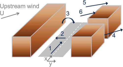
2. Across-Canyon Direct Dispersion. The direct dispersion of pollutants across the canyon by recirculating flow is represented by a simplified road source. For shallow canyons, with height-to-width ratio H/g <1, the dispersion direction is perpendicular to the canyon axis in the opposite direction to the component of upstream wind perpendicular to the canyon axis, representing a single recirculation cell. In deeper canyons, dispersion is considered in both directions across the canyon, in order to represent the more complex and less structured flow patterns, which can occur in these canyon geometries. The concentrations from this source only affect output points within the canyon. The source height is given by the road elevation plus an initial mixing height of 1 m, with an initial vertical spread of 1 m and initial horizontal spread of half the road width.

   An analytical integrated solution is used for dispersion from this source, based on flow divergence and vertical dispersion, due to the relatively short distances over which the dispersion is considered. Equation 2(2) $C_0=\frac{Q}{{\sigma }_{w}w}ln\frac{2U_y{H}_0+{\sigma }_W\left(y+\frac{w}{2}\right)}{2U_y{H}_0+{\sigma }_W\left(y-w_{incl}\right)}$(2) gives the expression for the ground-level concentration, at distance $y$ from the center of the road.

   (2) $C_0=\frac{Q}{{\sigma }_{w}w}ln\frac{2U_y{H}_0+{\sigma }_W\left(y+\frac{w}{2}\right)}{2U_y{H}_0+{\sigma }_W\left(y-w_{incl}\right)}$(2)

   where $Q$ is the emission rate, ${\sigma }_w$ is the vertical turbulence velocity, $w$ is the road carriageway width, $U_y$ is the across-canyon ground-level flow rate, $H_0$ is the initial mixing height for road sources (1 m) and $w_{incl}$ is the width of the road from which emissions affect the output height, given by

   (3) $w_{incl}=min\left(\frac{w}{2},y,y-\mathrm{\Delta }{y}_{Zop}\right)$(3)

   The variable $\mathrm{\Delta }{y}_{Zop}$, which is an estimate of the horizontal distance required for the plume to spread from its initial height $z_s$ and depth $H_0$ to the height of the output point, $z_{op}$, is defined by:

   (4) $\mathrm{\Delta }{y}_{Zop}=\frac{\left(z_{op}-z_s-2H_0\right)U_y\left(H_0\right)}{{\sigma }_W}$(4)

   The ground-level concentration is applied at output points at or below the source height $z_s$, plus twice the initial mixing height $H_0$. Above this, a vertical profile is applied, given by eq 5(5) $C=C_0\frac{\left(z_{op}-z_S+2H_0\right)}{4H_0}+\frac{Q}{{\sigma }_{W}w}\frac{z_{op}-z_S-2H_0}{4H_0}ln\left(\frac{y-w_{incl}}{y+\frac{w}{2}}\right)$(5) .

   (5) $C=C_0\frac{\left(z_{op}-z_S+2H_0\right)}{4H_0}+\frac{Q}{{\sigma }_{W}w}\frac{z_{op}-z_S-2H_0}{4H_0}ln\left(\frac{y-w_{incl}}{y+\frac{w}{2}}\right)$(5)

   For deeper canyons, with $H/g>$1, the dispersion across the street is represented by a weighted sum of concentrations calculated assuming the ground-level flow is in the opposite and same directions as the background flow. Further details are given in Appendix A.

3. Recirculation. The analytical solution for flow in a deep cavity driven by perpendicular flow across the opening gives a series of counter-rotating vortices, each of depth approximately equal to the cavity width. However, in more realistic street canyon flow situations, no more than 3 vortices have been observed (Murena et al. 2009). Hence, the formulation for the recirculation region component source concentration allows for up to three cells to cover the full depth of the canyon.

   The uppermost cell within the canyon is defined as extending from the minimum of the two canyon wall average building heights ($H_{min}=min\left(H_{avgL},H_{avgR}\right)$) to the maximum of these two heights ($H_{max}=max\left(H_{avgL},H_{avgR}\right)$). If one canyon wall is absent, this will be the only cell included. The lowest cell within the canyon is defined as extending from the ground up to $h_1=min\left(z_s+2H_0+g,H_{min}\right)$. In a shallow symmetric canyon, only the lowest cell will be included. In a deeper canyon, the middle cell is defined in the depth between $h_1$ and $H_{min}$.

   The concentration in the top recirculation cell is given by

   (6) $C_3=\frac{H_{max}-H_{min}}{g}\frac{Q}{g{\sigma }_3}$(6)

   Where ${\sigma }_3$ is a modified turbulence at the top of the top cell, representing additional mixing from vortex shedding around building tops, given by

   (7) ${\sigma }_3=\sqrt{\lambda {({\sigma }_u\left(H_{max}\right))}^2+{({\sigma }_w\left(H_{max}\right))}^2}$(7)
   (8) $\mathrm{w}\mathrm{h}\mathrm{e}\mathrm{r}\mathrm{e}\lambda =min\left(\frac{H_{max}-H_{min}}{g},1\right)$(8)

   The concentration in the middle cell is given by:

   (9) $C_2=C_3+max\left(\frac{H_{min}-h_1}{g},0\right)\frac{Q}{g{\sigma }_w\left(H_{min}\right)}$(9)

   While the concentration in the lowest cell is given by:

   (10) $C_1=C_2+min\left(1,\frac{H_{min}}{g}\right)\frac{Q}{g{\sigma }_w\left(h_1\right)}$(10)

   A linear smoothing is applied to the vertical profile of concentrations across the boundaries between cells, as described in Appendix A. In low to moderate aspect ratio canyons, a lateral profile is also applied to the recirculation in the lowest cell to represent the transition from direct across-canyon dispersion to recirculation; further details are given in Appendix A.

4. No-Canyon. The dispersion of pollutants through gaps between buildings in the canyon walls is represented by standard ADMS-Urban road source modeling, driven by upstream flow and contributing to output concentrations at output locations both within and outside the canyon. The source height is given by the road elevation plus an initial mixing height of 1 m, with an initial vertical spread of 1 m and initial lateral spread calculated from traffic-induced turbulence.

5. Canyon Top. The dispersion of pollutants out of the top of the canyon is represented by a volume source, where the source footprint coincides with the canyon area. The base of the volume source is defined at the minimum building height on the downstream side of the canyon. The volume source depth is calculated as the maximum of twice the road source initial mixing height ($H_0$) and the range of building heights on the downstream canyon wall. The volume source dispersion uses the standard ADMS-Urban modeling approach, driven by upstream flow at the source center height, and only contributes to concentrations at output locations outside the canyon.

6. Canyon End. The dispersion of pollutants out of the end of the canyon is only represented when the network mode for effects of connected canyons is in use. In this case, a volume source is defined at the downstream end of the network with footprint covering the downstream 20 m of the canyon. The source is ground-based, with a depth half of the smallest of the average canyon height, and the vertical spreading along the canyon length of material emitted at the upstream end of the canyon. The volume source uses the standard ADMS-Urban modeling approach, driven by upstream flow at the source center height, and contributing to output concentrations only at output locations outside the canyon, downstream of a line perpendicular to the downstream end of the canyon.

Source weightings

The component source weightings are determined by apportioning the total source strength $q$ between the components: $q_1$ for the along-canyon source; $q_2$ for the across-canyon source; $q_3$ for the recirculation region; $q_4$ for the non-canyon road source; $q_5$ for the canyon-top volume source; and $q_6$ for the canyon end volume source (only used in network mode).

Emissions from a road source can be separated into a fraction, $f_{out}$, that disperses freely out of the canyon (either over or through the gaps between the buildings) and the remainder, $1-f_{out}$, that stays initially trapped within the canyon. For tall canyons ($H/g\ge 1$), skimming flow effectively traps all emissions from those parts of the road source that are adjacent to buildings (Oke 1988) and so $f_{out}$ depends only on the canyon porosity:

(11) $f_{out}={\alpha }^{m}H/g\ge 1$(11)

where $m$ is the porosity power, with an empirically determined value of 2. $\alpha$ is the “overall porosity” of the canyon, taken as the minimum of ${\alpha }_L$ and ${\alpha }_R$ when the upstream wind is perpendicular to the canyon, and the mean of ${\alpha }_L$ and ${\alpha }_R$ when it is parallel. For intermediate values of $\mathrm{\Delta }\varphi ={\varphi }_c-{\varphi }_w$, where ${\varphi }_c$ is the canyon orientation and ${\varphi }_w$ the wind direction, $\alpha$ is given by:

(12) $\alpha =\mathrm{m}\mathrm{i}\mathrm{n}\left({\alpha }_L,{\alpha }_R\right){sin}^2\mathrm{\Delta }\varphi +\frac{1}{2}\left({\alpha }_L+{\alpha }_R\right){cos}^2\mathrm{\Delta }\varphi$(12)

For shallower canyons ($H/g<1$), wake interference becomes more prominent, which acts to increase $f_{out}$ as the aspect ratio decreases. This is accounted for by taking:

(13) $f_{out}=\frac{{\alpha }^m}{{\alpha }^m+\left(1-{\alpha }^m\right){\left(H/g\right)}^n}H/g<1$(13)

where $n$ is the aspect ratio power, with an empirically determined value of 0.5.

Here, the fraction that disperses freely out of the canyon is ascribed to the non-canyon component source, and the fraction that initially stays within the canyon is split between the along-canyon and across-canyon component sources, i.e.:

(14) $q_4=f_{out}q$(14)

(15) $q_1+q_2=\left(1-f_{out}\right)q$(15)

Note that for a road with no canyon walls, $q_4=q$ and the model results are identical to standard ADMS-Urban road source modeling, leading to a smooth transition between canyon and non-canyon source representation.

The relative strength of sources 1 and 2 is given by

(16) $\frac{q_1}{q_1+q_2}=\mathrm{m}\mathrm{a}\mathrm{x}\left(1-\gamma \mathrm{s}\mathrm{i}{\mathrm{n}}^2\mathrm{\Delta }\varphi ,0\right)$(16)

where $\gamma =\frac{1}{si{n}^2\left(\mathrm{\Delta }{\varphi }_{cr}\right)}=4$, corresponding to a critical wind direction difference ($\mathrm{\Delta }{\varphi }_{cr}$) value of 30° for the transition from along-canyon to across-canyon dispersion.

The material in the recirculation region (source 3) originates from the across-canyon dispersion (source 2) so $q_3=q_2$. Material reaches the top of the canyon either through dispersion along the canyon (source 1) or recirculation (source 3), so the strength of the canyon-top source (5) is given by $q_5=q_1+q_3$. These expressions conserve mass because the sources have different regions of influence: $q_5$ only affects output points outside the canyon while $q_1$, $q_2$ and $q_3$ only affect output points within the canyon. However, the trapping of emitted pollutants in the recirculation region can locally increase concentrations, representing delayed dispersion out of the canyon.

In network mode, some of the component source weightings are modified using additional canyon properties: $L_R$, the length of the road segment; $L_u$, the length of canyon upstream of the current segment; $L_t$, the along-canyon distance required for the material to disperse from the road surface to the top of the canyon, calculated from along-canyon wind speed, vertical turbulence, and average canyon height; and ${\gamma }_e$, the fraction of emissions leaving the canyon end, not channeled into another canyon.

A critical length scale $L_c$, representing the downstream distance for the maximum vertical dispersion within the canyon, is defined as

(17) $L_c=min\left(L_t,L_R+L_u\right)$(17)

The canyon-top source (5) emissions are reduced for canyons with insufficient upstream canyon length for emissions to have reached the canyon top:

(18) $if{L}_c>L_u,q_{5,network}=q_5-q_1\left(\frac{L_c-L_u}{L_R}\right)$(18)

In the most downstream segment of a canyon, the canyon end source (6) weighting is given by:

(19) $q_6={\gamma }_e\frac{L_c}{L_R}{q}_1$(19)

while for all other segments $q_6$ is zero. Source weightings $q_2,q_3$ and $q_4$ are unchanged. The source length for the along-canyon dispersion ($q_1$) is increased by the upstream canyon length, which can increase the relative strength of this source.

Additional considerations for asymmetric canyons

If no buildings are present on one side of the canyon, the wall height is set to zero and the porosity to unity. The “width” for this side of the canyon is set to 1.1 times the width on the side with non-zero height, in order to avoid a symmetric solution. The along-canyon source plume is only limited in width on a side with non-zero building height.

The overall porosity is calculated dependent on wind direction for use in source weighting calculations, as

(20) $\alpha =min\left({\alpha }_u,{\alpha }_d\right)si{n}^2\left({\varphi }_c-{\varphi }_w\right)+0.5\left({\alpha }_u+{\alpha }_d\right)co{s}^2\left({\varphi }_c-{\varphi }_w\right)$(20)

where subscripts $u$ and $d$ indicate upstream and downstream properties. For wind directions very close to parallel with the canyon axis, the concept of upstream and downstream sides is not well defined; for these cases, average canyon properties are used instead.

If the downstream canyon wall is higher than the upstream wall, the across-canyon source weighting, $q_2$, is reduced by the factor $max\left(\left(H_d-H_u\right)/H_d,0.3\right)$, with a corresponding increase in the non-canyon source strength $q_4$. Similarly, if the upstream wall is higher than the downstream wall, the along-canyon source weighting, $q_1$, is reduced by the factor $\left(H_d-H_u\right)/H_u$, again with a corresponding increase in $q_4$.

Comparison between basic and advanced canyon models

The basic canyon model has been incorporated within ADMS-Urban since that model was developed (Owen et al. 2000). It is based on OSPM and details of the formulation are available in an ADMS-Urban Technical Specification document (CERC 2017b). The fundamental differences between the advanced canyon model described in this paper and the basic canyon model are summarized in Table 2.

Table 2. Overview of differences between the advanced and basic canyon models

Model feature	Advanced canyon	Basic canyon
Urban canopy flow adjustment	In-canyon urban canopy flow field derived from canyon heights and widths	Urban canopy flow can be accounted for by use of the urban canopy flow module
Canyon porosity	Smooth transition between fully enclosed canyons (zero porosity) and open roads (porosity of unity)	Only accounts for fully enclosed canyons
Region of influence	Influences concentrations both within and outside the street canyon	Only influences concentrations inside the canyon
Vertical variation	Concentrations vary vertically	No change in concentrations with height
Road carriageway definition	Road carriageway and canyon widths are defined separately and the model accounts for different canyon widths on each side, allowing for the presence of pedestrian areas, central reservations etc.	The road carriageway is assumed to have the same width as the canyon
Canyon asymmetry	Accounts for canyon asymmetry	Canyons are assumed to be symmetric

Model validation datasets description

The advanced canyon model is evaluated using measured concentration data from the “Optimisation of modelling methods for traffic pollution in streets” (TRAPOS) project, specifically from Jagtvej (Copenhagen, Sweden), Goettingerstrasse (Hanover, Germany) and Schildhornstrasse (Berlin, Germany), and routine measurement data from 42 monitoring sites in London, UK (LAQN, 2017). In order to understand the importance of accounting for street canyons in detail, model predictions when no canyon has been modeled, and also with the application of the basic canyon method, have been evaluated alongside the advanced canyon results.

Figure 2 shows each of the TRAPOS sites. For each site, the measurement location is shown on a map, and locations of the meteorological and background pollutant concentration measurement sites are indicated if they are in the vicinity of the street canyon. For each location, the inset photograph shows the type of buildings that make up the canyon. The corresponding wind rose, showing the distribution of wind speed and direction during the study, is also shown. Detailed vehicle fleet and speed data associated with these studies are unavailable, which limits the accuracy of traffic emission calculations. The Handbook Emission Factors for Road Transport (HBEFA, Keller et al. 2017) database has been used to calculate emissions of hydrocarbons, CO, NOx, and NO₂, with estimated road type, speed limit, and traffic situation (congestion level) inputs. Concentrations of CO, NOx, and NO₂ were recorded during the TRAPOS campaign. However, due to uncertainties associated with the proportion of NOx that is NO₂, and suitable urban background O₃ concentrations, model evaluation in terms of NO₂ predictions has not been presented here. There are eight years of data available for the Jagtvej site (1994–2002), although for brevity data for only the first year (1994) has been presented in this paper; the Goettingerstrasse campaign dataset covers one year (1995) as does the Schildhornstrasse campaign (1994).

Figure 2. TRAPOS site locations and corresponding wind roses a) Jagtvej with the location of the meteorological and air quality monitoring stations shown; b) Goettingerstrasse with the meteorological and air quality monitoring station shown c) Schildhornstrasse with the air quality monitoring station shown. © OpenStreetMap (and) contributors; CC-BY-SA, © 2020 Google, © 2019 Google Data, © 2009 GeoBasis. Please refer to the online version for color figures

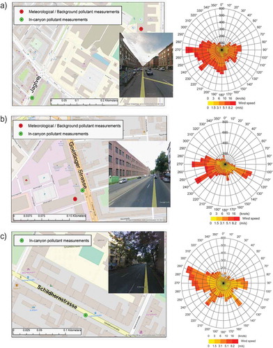
Jagtvej has traffic flows of around 22,000 vehicles per day, with carriageway width 13.6 m, a canyon 25 m wide and buildings on both sides around 18 m tall, giving a canyon height/width ratio of 0.72. The road aligns approximately 30⁰ clockwise from the north and the monitoring site is located adjacent to the south-easterly side of the road, 5.7 m from the canyon wall, and with an inlet height of 3.5 m. Weekday, Saturday, and Sunday profiles of traffic flow data are provided as overall total cars, vans, trucks, and buses, separately for July (a holiday month in Denmark) and months other than July. HBEFA emission factors were selected for a “distributor/secondary” road with a speed limit of 50 km/hr. HBEFA does not include specific factors for Denmark, so factors for Sweden were used. The traffic situation was defined as “free-flow” for hours with total traffic flow below 1500 vehicles or “heavy” for hours with higher traffic flow. Local hourly background concentration data for NOx and CO are supplied from a Copenhagen University building rooftop site 0.5 km to the North East of the study site. Diurnal average profiles for weekdays, Saturdays, and Sundays are used to fill the missing hours where gaps occur in the background data series. Hourly measured meteorological data comprising wind speed, wind direction, global radiation, and temperature are available from the University building rooftop; these data were used directly as input to the ADMS meteorological pre-processor with the exception of the global radiation which was used to derive incoming short-wave radiation and cloud cover for input to the model. The wind data show a mixture of cross-canyon and along-canyon directions.

The Goettingerstrasse site has an overall traffic flow of around 30,000 vehicles per day. Each of the four lanes has carriageways 3.75 m wide while the overall canyon is 25 m wide and has average building heights of around 21 m, giving a height/width ratio of 0.84. The road is aligned approximately 15 degrees anticlockwise from North. The monitoring site is located close to the canyon wall on the south-westerly side of the street with an inlet height of 1.5 m. Hourly traffic counts of “long” and “short” vehicles are provided for each lane. For use in HBEFA, the “short” vehicles were apportioned into 83% cars and 17% vans and “long” vehicles into 70% trucks and 30% buses based on traffic data from Schildhornstrasse. HBEFA emission factors for Germany were selected for a “distributor/secondary” road with a speed limit of 50 km/hr. The traffic situation was defined as “free-flow” for hours with total traffic flow below 1750 vehicles or “heavy” for hours with higher traffic flow. Local hourly background concentration data for NOx and CO are supplied from a rooftop site; as for Jagtvej, diurnal average background concentrations are used to fill in for missing data. Hourly measured meteorological data are supplied from a nearby rooftop comprising wind speed, wind direction, net radiation, and temperature. For input to ADMS-Urban, expressions for solar radiation, cloud cover, and net radiation were used to back-calculate appropriate input values of solar radiation and cloud cover. The distribution of wind data for this study is dominated by across-canyon wind directions.

The Schildhornstrasse site is an access route to the city motorway carrying around 45,000 vehicles per day. The road carriageway width is 18.2 m while the total canyon width is 26 m and the average canyon height 21 m, giving a height/width ratio of 0.79. The monitoring site is in the parking lane adjacent to the south-westerly side of the road, with inlet height 2.5 m. Diurnal profiles of cars, vans, trucks, and buses are provided for weekdays, Saturdays, and Sundays. HBEFA emission factors for Germany were selected for a trunk/city road with a speed limit of 50 km/hr. The traffic situation was defined as “free-flow” for hours with total traffic below 1500 vehicles, “heavy” for hours with traffic flow between 1500 and 4000 vehicles, and “saturated” for hours with higher traffic flow. Hourly urban background concentration data of NOx and CO are available from a continuous monitoring station on Lentzeallee. Hourly measured meteorological data from a University building rooftop site 0.5 km to the North East of the site are available, comprising wind speed, wind direction, global radiation, and temperature; for input to ADMS, the global radiation data were converted to solar radiation as for Jagtvej. The wind data for this study are predominantly along-canyon wind directions.

ADMS-Urban model validation using data from reference monitors in London for the year 2012 has been described fully in Hood et al. (2018); the ADMS-Urban canopy flow model and the advanced canyon model were used in that study, with canyon parameters calculated using the tool and data described in Jackson et al. (2016). The “standalone” model configuration is used again here, to compare the results of the application of the advanced canyon model alongside results from the application of the basic canyon model, and also no canyon modeling. A brief summary of the data used in the study is given in Table 9 in Appendix A. The focus is on the 42 monitoring sites which have adequate data coverage for at least two of NO_x, NO₂, and O₃, of which 27 are classified as “near-road”. The maximum height/width ratio value for the near-road sites is 1, while 12 sites with height/width values greater than 0.35 and a porosity of less than 0.5 have been classed as “strong canyons”. Within this dataset, the Marylebone Road “supersite” (Green 2002) has been selected for a more detailed study.

Results

Model evaluation for no canyon, basic canyon, and advanced canyon configurations is calculated for each study using the Model Evaluation Toolkit (Stidworthy et al. 2013). The statistics defined in Equations 21(21) $Fb=\frac{\bar{M}-\bar{O}}{0.5\left(\bar{O}+\bar{M}\right)}$(21) to 25 are used to evaluate the modeled concentrations $M$ in relation to the observed concentrations $O$, where: $n$ is the number of pairs of modeled and observed concentrations; a bar indicates the mean value (e.g., $\bar{M}$); and a subscript indicates a single parameter value ranked between unity and $n$ (e.g. $M_i$). Mean observed and modeled concentrations are presented alongside mean bias, $\bar{M}-\bar{O}$, and the ratio of the standard deviation of modeled concentrations, ${\sigma }_M$, to the standard deviation of observed concentrations, ${\sigma }_O$.

Fractional bias ($Fb$) is a measure of the mean difference between the modeled and observed concentrations:

(21) $Fb=\frac{\bar{M}-\bar{O}}{0.5\left(\bar{O}+\bar{M}\right)}$(21)

Normalized mean square error ($NMSE$) is a measure of the mean difference between matched pairs of modeled and observed concentrations:

(22) $NMSE=\frac{\overline{{\left(M-O\right)}^2}}{\overline{MO}}$(22)

Pearson’s Correlation coefficient ($R$) is a measure of the extent of a linear relationship between the modeled and observed concentrations:

(23) $R=\frac{1}{n-1}\sum _{i=1}^n\left(\frac{M_i-\bar{M}}{{\sigma }_M}\right)\left(\frac{O_i-\bar{O}}{{\sigma }_O}\right)$(23)

Fraction of modeled hourly concentrations within a factor of two of observations ($Fac2$) is given by the fraction of model predictions that satisfy

(24) $0.5\le \frac{M_i}{O_i}\le 2.0$(24)

The statistic used to quantify overall model performance is the Index of Agreement, IoA (Willmott, Robeson, and Matsuura 2012) given by:

(25) $\mathrm{I}\mathrm{o}\mathrm{A}=\left\{\begin{array}{c}1-\frac{{\sum }_i\left|M_i-O_i\right|}{2{\sum }_i\left|O_i-\bar{O}\right|},\sum _i\left|M_i-O_i\right|\le 2\sum _i\left|O_i-\bar{O}\right|\\ \frac{2{\sum }_i\left|O_i-\bar{O}\right|}{{\sum }_i\left|M-O_i\right|}-1,\sum _i\left|M_i-O_i\right|>2\sum _i\left|O_i-\bar{O}\right|\end{array}\right.$(25)

The IoA spans between −1 and +1, with values approaching +1 representing better model performance.

Following Chang and Hanna (2004), model performance has been assessed visually using NMSE-Fb plots, in which points close to the origin indicate good performance. The openair tool (Carslaw and Ropkins 2012) has also been used to generate plots that assist in understanding the model’s ability to capture concentration variation in relation to governing parameters such as wind speed and wind direction; also, openair facilitates inspection of model performance categorized by other parameters such as time, and concentration magnitude.

TRAPOS sites

For the three TRAPOS studies, model evaluation statistics are presented in Table 3 for NOx and Table 4 for CO. Jagtvej results for 1994 have been presented; other years show very similar behavior. In these tables, statistics shown in italics indicate the best performance whilst bold shows better performance than the other models by at least 5%. In all cases, the advanced canyon model demonstrates the best performance, and predictions of NOx are generally more accurate than CO. For CO both average concentrations and ${\sigma }_M/{\sigma }_O$ values are under-predicted consistent with the emissions being under-estimated.

Table 3. Model evaluation statistics for NOx for the TRAPOS studies; statistics shown in italics indicate the best performance whilst bold shows better performance than the other models by at least 5%

Site	Model	Mean (ppb)	Fb	${\sigma }_{\mathrm{M}}/{\sigma }_{\mathrm{O}}$	NMSE	R	Fac2	IoA
Jagtvej	Observed	85.9	0.000	1.00	0.000	1.000	1.000	1.000
	No Canyon	34.6	−0.852	0.36	2.357	0.625	0.505	0.565
	Basic Canyon	60.0	−0.356	0.56	0.591	0.846	0.789	0.717
	Advanced Canyon	73.8	−0.152	0.80	0.229	0.898	0.933	0.816
Goettingerstrasse	Observed	157.3	0.000	1.00	0.000	1.000	1.000	1.000
	No Canyon	75.4	−0.705	0.74	1.959	0.214	0.362	0.395
	Basic Canyon	117.7	−0.288	0.75	0.352	0.796	0.782	0.693
	Advanced Canyon	172.7	0.093	1.33	0.244	0.861	0.950	0.742
Schildhornstrasse	Observed	130.6	0.000	1.00	0.000	1.000	1.000	1.000
	No Canyon	60.5	−0.734	0.54	1.849	0.373	0.378	0.474
	Basic Canyon	102.0	−0.245	0.68	0.376	0.791	0.829	0.709
	Advanced Canyon	139.5	0.066	1.05	0.182	0.859	0.918	0.774

Table 4. Model evaluation statistics for CO for the TRAPOS studies; statistics shown in italics indicate the best performance whilst bold shows better performance than the other models by at least 5%

Site	Model	Mean (ppb)	Fb	${\sigma }_{\mathrm{M}}/{\sigma }_{\mathrm{O}}$	NMSE	R	Fac2	IoA
Jagtvej	Observed	1.43	0.000	1.00	0.000	1.000	1.000	1.000
	No Canyon	0.14	−1.644	0.13	14.933	0.390	0.010	0.315
	Basic Canyon	0.36	−1.194	0.25	4.074	0.807	0.106	0.431
	Advanced Canyon	0.48	−0.994	0.40	2.294	0.860	0.105	0.495
Goettingerstrasse	Observed	1.73	0.000	1.00	0.000	1.000	1.000	1.000
	No Canyon	0.73	−0.807	0.42	1.657	0.309	0.457	0.386
	Basic Canyon	0.87	−0.661	0.43	1.007	0.637	0.539	0.473
	Advanced Canyon	1.04	−0.496	0.56	0.602	0.723	0.674	0.559
Schildhornstrasse	Observed	1.96	0.000	1.00	0.000	1.000	1.000	1.000
	No Canyon	0.52	−1.162	0.30	3.949	0.395	0.279	0.387
	Basic Canyon	0.76	−0.883	0.35	1.899	0.737	0.347	0.488
	Advanced Canyon	0.97	−0.671	0.47	1.003	0.855	0.531	0.578

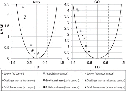
Figure 3 shows NMSE-Fb plots for NOx and CO, for all studies; the NOx plot clearly shows how modeling street canyons using either the basic or the advanced canyon methods significantly improves model performance compared to when no canyon is considered, whereas the CO plot is strongly influenced by inaccuracies in the emission data (low Fb). All subsequent discussion of model evaluation using the TRAPOS dataset has been restricted to the NOx concentration data due to poor specification of CO emissions.

Figure 3. Graphical representation of model evaluation statistics for NOx (left) and CO (right) for TRAPOS studies for each of the no canyon, basic canyon and advanced canyon configurations. Note that the plots use different vertical scales and the Jagtvej no canyon result for CO is outside the axis limits

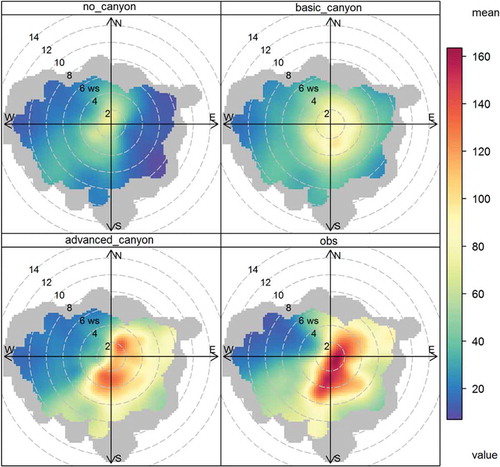
Polar plots are a useful graphical tool for visually comparing the variation of concentrations with wind speed and direction predicted by a model with those measured at a site. Figure 4 shows the polar plots at the Jagtvej monitor for each of the model configurations (no canyon, basic canyon, advanced canyon) alongside the observed data; in order to focus on the most reliable results, only cases where at least five data points have been included in the wind conditions bin are displayed. There is a much greater similarity between the concentration distribution for the advanced canyon model and the observations than either the basic canyon or the no canyon case, both in terms of concentration magnitude and spatial spread. The advanced canyon and observation data indicate high concentrations when winds range between approximately 30⁰ and 210⁰; since the road is aligned at an angle of 30⁰ clockwise from the north and the monitor is located on the easterly side of the road (Figure 2a), this concentration distribution indicates that the flow recirculation source component is important. The observations show high concentrations for a range of wind speeds when the flow is aligned along the road, suggesting that the channeling of flow is also a dominating factor in this canyon; the model along-canyon source component replicates this.

Figure 4. Polar concentration NOx (ppb) plot for Jagtvej with wind speed on the radial axis, and wind direction on the azimuth angle: No canyon (top left), Basic canyon (top right), Advanced canyon (bottom left), and observations (bottom right). Combinations of wind direction and wind speed which occur for fewer than 5 hours in the year are grayed out. Please refer to the online version for color figures

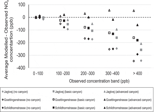
Whilst the model evaluation statistics presented in Tables 3 and 4 are useful in assessing overall model performance, the model’s ability to replicate high concentrations is important in terms of the application of the model for assessment and planning purposes where reliable air quality limit exceedance calculations are required. Figure 5 presents NOx frequency scatter plots for each of the no canyon, basic canyon, and advanced canyon cases for the Schildhornstrasse study, as generated by openair. These plots, in which the color range indicates the density of data points, clearly show that the advanced canyon model is better able to predict the high concentration values compared to the no canyon and basic canyon cases. To quantify this improvement in model performance in terms of prediction of the high concentration values, the modeled data for all three TRAPOS sites have been analyzed by considering data within a series of observed concentration bands (0– 100, 100– 200 ppb, etc.). Averages of the hourly bias values within each band have been calculated for each model configuration and plotted graphically in Figure 6 (using identifiers consistent with Figure 3). At all sites, for concentrations above 200 ppb, the under-prediction by the no canyon configuration is approximately 70%; for the basic canyon, the under-prediction is approximately 35% for Goettingerstrasse and Schildhornstrasse, but closer to 50% for Jagtvej. The advanced canyon model demonstrates good performance for high concentrations at Goettingerstrasse and Schildhornstrasse but some underprediction (40%) at Jagtvej, demonstrating that the advanced canyon model can predict more accurate concentrations than either of the other methods for high concentration values. Figure 6 also demonstrates that urban morphology causes the high pollutant concentrations. That is, for the high observed concentrations, the no canyon configuration under-predicts measured values by approximately a factor of three, indicating that if the same source was located in an open area, the high concentrations would be significantly reduced.

Figure 5. Frequency scatter plots of NOx (ppb) for Schildhornstrasse for each model configuration: No canyon (left), Basic canyon (middle), Advanced canyon (right); color range indicates the number of data points within each hexagonal bin; plot generated using openair functions. Please refer to the online version for color figures

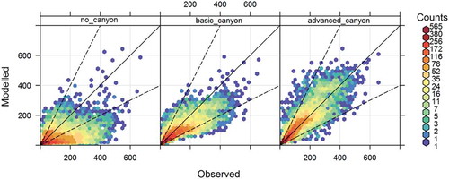
Figure 6. Average difference between observed and calculated NOx concentrations for each TRAPOS site and each of the no canyon, basic canyon and advanced canyon model configurations, binned according to observed concentrations

Another informative graphical evaluation assessment facilitated by openair is the inspection of average temporal profiles. Figure 8 in Appendix A compares the average diurnal, monthly, and daily NOx concentrations for the three model configurations to the observations. As indicated by the statistics and graphs already discussed, the advanced canyon model demonstrates better performance than either the no canyon or basic canyon model configurations.

London sites

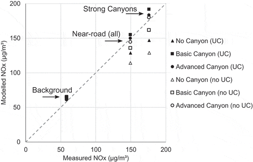
The London modeling evaluation statistics are presented in Tables 5, 6 and 7 for NOx, NO₂, and O₃, respectively, for all background sites, all near-road sites, and near-road sites with “strong canyons” (height/width ratio greater than 0.35 and porosity less than 0.5). As for Tables 3 and 4, the statistics shown in italics indicate the best performance, whilst bold shows better performance than the other models by at least 5%. One consequence of considering the large number of monitor locations available in London is that the model configuration has not been refined on a site-by-site basis, although the most important parameters such as monitor to road carriageway edge distance have been checked. Further, very few of the LAQN sites are located in well-defined street canyons; sites are often at junctions or may be influenced by other local source terms, for example, bus stops. These complexities somewhat reduce both the differences in the performances of the different models and their accuracy compared to the TRAPOS evaluation for NOx. For instance, for all three of the TRAPOS sites, NOx correlation values for the advanced canyon configuration exceed 0.85, and the number of points within a factor of two of the observed is over 0.9; in contrast, both these statistics are approximately 0.6 for the advanced canyon configuration for the strong canyon subset of NOx data values; the number of modeled concentrations within a factor of two of the observed concentrations is higher (0.82) when NO₂ is evaluated. However, with the exception of the background sites where differences are marginal, the London dataset demonstrates performance that is consistent with the TRAPOS evaluation, i.e., overall, the advanced canyon model performs better than other model configurations, with the IoA, NMSE, and correlation being higher for the advanced canyon configuration for each of the pollutants and site subsets.

Table 5. Model evaluation statistics for NOx for continuous monitoring sites in London

Site type	Model	Mean (µg/m^3)	Fb	${\sigma }_{\mathrm{M}}/{\sigma }_{\mathrm{O}}$	NMSE	R	Fac2	IoA
Strong canyons	Observed	176.2	0.000	1.00	0.000	1.000	1.000	1.000
	No Canyon	147.0	−0.181	0.84	1.020	0.428	0.605	0.563
	Basic Canyon	191.5	0.083	0.98	0.677	0.554	0.655	0.575
	Advanced Canyon	183.4	0.040	0.96	0.601	0.618	0.605	0.617
Near-road (all)	Observed	149.6	0.000	1.00	0.000	1.000	1.000	1.000
	No Canyon	128.5	−0.152	0.85	0.890	0.515	0.661	0.599
	Basic Canyon	154.9	0.035	0.97	0.662	0.598	0.697	0.608
	Advanced Canyon	149.6	0.000	0.93	0.623	0.625	0.699	0.626
Background	Observed	58.7	0.000	1.00	0.000	1.000	1.000	1.000
	No Canyon	65.2	0.104	1.03	0.858	0.620	0.743	0.622
	Basic Canyon	65.4	0.108	1.03	0.857	0.620	0.741	0.620
	Advanced Canyon	61.6	0.048	0.95	0.860	0.610	0.738	0.631

Table 6. Model evaluation statistics for NO₂ for continuous monitoring sites in London

Site type	Model	Mean (µg/m^3)	Fb	${\sigma }_{\mathrm{M}}/{\sigma }_{\mathrm{O}}$	NMSE	R	Fac2	IoA
Strong canyons	Observed	70.2	0.000	1.00	0.000	1.000	1.000	1.000
	No Canyon	60.1	−0.155	0.90	0.489	0.442	0.743	0.544
	Basic Canyon	74.1	0.054	1.06	0.345	0.567	0.793	0.560
	Advanced Canyon	74.7	0.062	1.01	0.293	0.617	0.821	0.588
Near-road (all)	Observed	60.8	0.000	1.00	0.000	1.000	1.000	1.000
	No Canyon	55.2	−0.097	0.96	0.385	0.543	0.796	0.580
	Basic Canyon	63.3	0.040	1.09	0.306	0.629	0.829	0.588
	Advanced Canyon	64.7	0.062	1.02	0.277	0.638	0.828	0.590
Background	Observed	35.4	0.000	1.00	0.000	1.000	1.000	1.000
	No Canyon	37.0	0.043	1.06	0.272	0.681	0.837	0.637
	Basic Canyon	37.1	0.045	1.07	0.272	0.681	0.836	0.636
	Advanced Canyon	36.0	0.016	1.02	0.275	0.668	0.830	0.638

Table 7. Model evaluation statistics for O₃ for continuous monitoring sites in London

Site type	Model	Mean (µg/m^3)	Fb	${\sigma }_{\mathrm{M}}/{\sigma }_{\mathrm{O}}$	NMSE	R	Fac2	IoA
Strong canyons	Observed	24.5	0.000	1.00	0.000	1.000	1.000	1.000
	No Canyon	27.9	0.132	0.96	0.453	0.685	0.522	0.632
	Basic Canyon	25.3	0.032	0.93	0.395	0.735	0.562	0.678
	Advanced Canyon	23.7	−0.030	0.94	0.339	0.788	0.597	0.715
Near-road (all)	Observed	26.9	0.000	1.00	0.000	1.000	1.000	1.000
	No Canyon	30.6	0.127	1.04	0.297	0.756	0.610	0.665
	Basic Canyon	29.4	0.087	1.02	0.290	0.761	0.618	0.677
	Advanced Canyon	27.5	0.023	0.99	0.285	0.767	0.628	0.692
Background	Observed	35.5	0.000	1.00	0.000	1.000	1.000	1.000
	No Canyon	34.7	−0.020	0.95	0.212	0.775	0.696	0.710
	Basic Canyon	34.7	−0.021	0.95	0.212	0.775	0.696	0.710
	Advanced Canyon	35.0	−0.013	0.95	0.214	0.772	0.694	0.708

In contrast to the TRAPOS studies, where the advanced canyon mean concentrations were always higher than the other configurations, for London, the basic canyon configuration predicts a higher mean than the advanced canyon for NOx. This is a consequence of the advanced canyon better representing dispersion out of incomplete or porous canyons than the basic canyon, which treats many of these cases as full canyons with no porosity. Taking this further, inspection of the statistics associated with the background sites shows that although for the majority of statistics (NMSE, R, Fac2) the behavior of the model at the background sites differs little between the model configurations, the advanced canyon model predicts generally lower (and more accurate) NOx and NO₂ concentrations at the background sites; this is likely explained by the use of the canyon-top source, which elevates the source of the fraction of canyon emissions which are dispersed outside the canyon; as a consequence O₃ concentrations are higher using the advanced canyon model at background sites.

The Marylebone Road “supersite” in London has been the subject of a number of studies as the site records a wide range of pollutants (Green 2002) and is adjacent to a very busy road. Figure 9 in Appendix A shows the polar concentration plot similar to the one shown in Figure 4 for the TRAPOS study. This figure again demonstrates that the advanced canyon model is much better at representing the spread of observed concentration values with wind speed and wind direction compared to the other model configurations.

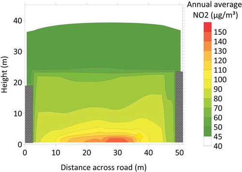
Having demonstrated that the advanced canyon model can be used to predict concentrations at measurement locations within street canyons, the model can then be applied for policy, planning, and assessment purposes, for example, air pollutant concentrations on building facades are modeled for housing development assessments. Figure 7 shows a vertical slice of modeled annual average NO₂ concentrations in the vicinity of the Marylebone Road supersite. This figure highlights many aspects of the advanced canyon formulation, for example, the model accounts for each road carriageway separately, in addition to the pavements (no emissions) and canyon walls; concentrations decrease with height, with the “in-canyon” concentrations being restricted to the maximum height of the buildings on either side of the road; and there is a smooth transition to the above-canyon concentration, which results from the canyon-top source. The Marylebone Road annual average NO₂ concentration measurement is shown on the plot (diamond symbol), and the observed value agrees well with the modeled concentration at the monitor location.

Figure 7. Annual average vertical cross-sectional NO₂ concentration contour plot (µg/m³) for Marylebone Road (2012) modeled using the advanced canyon model; diamond symbol overlaid on the modeled concentrations at coordinates (37.0 m, 2.5 m) represents the location and magnitude of the Marylebone Road measurement. Please refer to the online version for color figures

Discussion

This paper presents an evaluation of a new street canyon pollution dispersion model that has been implemented in the street-level resolution ADMS-Urban air quality model. The advanced street canyon model formulation has been described in detail. Two air quality measurement datasets have been used for the evaluation of the model. The first comprises data from the TRAPOS project, in which a single measuring station was installed in each of three street canyons recording hourly NOx and CO concentration data for at least one year; meteorological and background pollutant measurement data were available in addition to traffic activity data for emission estimation. The second dataset comprises NOx, NO₂, and O₃ air pollutant measurement data from the extensive London Air Quality Network and an ADMS-Urban model configuration for London that has been discussed in earlier work (Hood et al. 2018). Different model configurations have been used to represent the street canyons for both datasets, specifically: no canyon, basic canyon, and the new advanced canyon representations. The model evaluation exercise has involved the calculation of a range of statistics in addition to graphs and plots that have been used to demonstrate the agreement between the measured and modeled pollutant concentrations. As the London dataset includes measurements from urban background sites as well as near-road sites that are not located within street canyons, the results have been categorized according to site type.

The results of the model evaluation exercise clearly demonstrate the improvement in the predictions of the advanced canyon over the basic canyon modeling approach. For the TRAPOS study, the advanced canyon model demonstrates good performance for NOx with correlations greater than 0.85 and the proportion of modeled hourly average concentrations within a factor of two of the observed concentrations being greater than 0.9 at all sites; for CO, the advanced canyon performs better than either of the other model configurations, but overall performance is affected by large uncertainties in the CO emission estimates. The TRAPOS sites are all fairly shallow canyons with low porosity, and there is a strong influence of the street canyon geometry on the resultant concentrations. For these sites, it is likely that the allowance for the presence of pedestrianized areas/pavements at the side of roads in the advanced canyon model, restricting emissions to the locations of the road lanes, significantly improves model performance in comparison to the basic canyon, where the road carriageway and hence the location of emissions is assumed to have the same width as the canyon. For the London evaluation, where a wider range of site types has been considered, the model has been assessed in terms of its ability to calculate both dispersion and chemistry within the canyon, as NOx, NO₂, and O₃ are evaluated. The London evaluation demonstrates that the advanced canyon model not only accounts for dispersion but also local scale chemistry within the canyon. In general, the subset of sites that have been categorized as “strong canyons” have higher porosity compared to the TRAPOS sites. In consequence, average NOx concentrations predicted by the advanced canyon are lower than the corresponding predictions from the basic canyon configurations because the latter formulation does not account for canyon porosity. For NO₂, the differences between mean concentrations predicted by the basic canyon and advanced canyon are relatively small, but there is a noticeable improvement in correlation and the number of modeled concentrations within a factor of two of the observed concentrations for the strong canyon case.

In addition to the complex flows that occur locally within street canyons, urban morphology strongly influences wind and turbulence within the urban area at the neighborhood scale (scale of a few hundred meters). The spatial variation of building density and heights within a city generates flow field structure on this scale; this is modeled in ADMS-Urban using the urban canopy module (CERC 2017c; Hood et al. 2014). Accounting for wind flow variations within the urban canopy leads to reduced wind speeds in highly built-up areas and hence higher concentrations due to local sources. In this study such effects are included in the London runs but not the TRAPOS runs. It is of note that within the advanced street canyon model the vertical profile of wind speed is modified using a similar approach to that used for the urban canopy flow, but using canyon height rather than displacement height as the key vertical length scale to create a more locally representative flow field. The effects of the urban canopy flow model on concentrations of NOx for the no canyon, basic canyon, and advanced canyon cases are shown in Figure 10. These show that the use of the urban canopy option has much greater influence on modeled concentrations for the no canyon and basic canyon model cases compared to the advanced canyon, since these models have no local adjustment of the flow when the urban canopy model is not applied; thus, use of the urban canopy model for the London runs presented has tended to diminish the difference in the performances as compared to TRAPOS results, in particular improving the basic canyon (OSPM) model performance.

Finally, we note that the majority of air quality measurements are recorded near ground level. In order to comprehensively evaluate the performance of the advanced street canyon model, comparison of air quality measurements at elevated receptors is required, in addition to evaluation in deeper street canyons. The authors are collaborating with institutions in China in order to generate measurement datasets that will allow this type of model assessment in the future.

Acknowledgments

The authors would like to acknowledge: the Hong Kong Environmental Protection Department for funding the initial development of the advanced canyon module within ADMS-Urban; the European Commission’s Training and Mobility of Researchers Programme (TMR) within the framework of the European Research Network on “Optimisation of Modelling Methods for Traffic Pollution in Streets”, for funding the generation of the TRAPOS dataset; and to UK NERC for funding the CUREAIR project under grant NE/M002381/1, during which the London 2012 ADMS-Urban model configuration for London was developed.

Disclosure statement

No potential conflict of interest was reported by the authors.

Additional information

Funding

This work was supported by the Natural Environment Research Council [NE/M002381/1]; Hong Kong Environmental Protection Department.

Notes on contributors

Christina Hood

Christina Hood, MEng, Ph.D. is senior consultant at Cambridge Environmental Research Consultants in Cambridge, UK. She received her mechanical engineering undergraduate degree from the University of Cambridge. Christina obtained her PhD in the field of bioengineering, specifically respiratory gas flow modelling, from Imperial College London. At CERC, Christina works on application, development and assessment of local and regional scale atmospheric dispersion models.

Jenny Stocker

Jenny Stocker, BA, MSc, Ph.D. is principal consultant at Cambridge Environmental Research Consultants in Cambridge, UK. She received her undergraduate degree from the University of Oxford. Her Master’s degree and PhD were awarded by the University of Manchester in the field of fluid mechanics. At CERC, Jenny manages a range of projects involving the application, development and evaluation of meteorological and atmospheric dispersion models.

Martin Seaton

Martin Seaton, MA, MMath, Ph.D. is a principal consultant at Cambridge Environmental Research Consultants in Cambridge, UK. He received his undergraduate degree and PhD in applied mathematics from the University of Cambridge. At CERC, Martin oversees the development of scientific model code and documentation for the Atmospheric Dispersion Modelling System (ADMS) suite of air dispersion models.

Kate Johnson

Kate Johnson, MSc, is a senior consultant at Cambridge Environmental Research Consultants in Cambridge, UK. She graduated from Reading University with a Master’s degree in Weather, Climate and Modelling in 1994 and has worked at CERC as an environmental consultant since graduation. Her specialities include processing environmental data in an exacting way, modelling urban air quality and model evaluation.

James O’Neill

James O’Neill, MMath, MSc, Ph.D. is a senior consultant at Cambridge Environmental Research Consultants in Cambridge, UK. He received his undergraduate degree in mathematics from the University of Nottingham and subsequently obtained a Master's degree in applied meteorology and climatology at the University of Birmingham. His PhD is from the University of Birmingham in the topic of turbulence parameterisations for large-eddy simulation of neutral atmospheric flows. At CERC, James works in scientific software development.

Lewis Thorne

Lewis Thorne, MEng, is a graduate in Chemical Engineering from the University of Cambridge, 2020. He worked at CERC on model validation during a summer vacation in 2018. His interests include climate change mitigation and sustainable technologies.

David Carruthers

David Carruthers, BA, Ph.D. is a Technical Director of CERC with broad expertise in atmospheric science and complex atmospheric boundary layer processes in particular. He has overall responsibility for the development of CERC software including the different versions of the Atmospheric Dispersion Modelling System (ADMS), and has also directed many projects in air quality assessment both in the UK and internationally. His expertise has been recognised in his membership of the UK Government’s Air Quality Expert Group (AQEG). David is currently an Associate Editor of JA&WMA.

Appendix A

Network mode

When using network mode, the road (non-canyon and canyon) connections are analyzed to determine the possible routes that emissions within the network can take before escaping from the canyons.

During the dispersion calculations, for a given meteorological condition (wind direction) and canyon segment, the length of canyon upstream of that segment, $L_u$, and the fraction of emissions leaving the segment end not channeled into another canyon, ${\gamma }_e$, are calculated.

${\gamma }_e$ is taken as the fraction of downstream connecting segments that are not canyons, and is set to 1 if there are no connecting segments at all. ${\gamma }_e$ will be zero for any canyon segment that is not the most downstream segment of that canyon.

$L_u$ is calculated using the following iterative process:

• If the current segment is not the most upstream segment of that canyon, add the upstream-projected length of the next upstream segment to the value of $L_u$ of the upstream segment.

• If the current segment is the most upstream segment of that canyon, then for each upstream-connecting canyon, add the upstream-projected length of the connecting segment to the value of $L_u$ of the connecting segment and divide by the number of downstream-connected roads (canyon or non-canyon) if there is more than one (i.e., partition the upstream length, and therefore the emissions, from that connecting canyon equally between its downstream roads).

A user-definable maximum value (with a default of 300 m) is applied to $L_u$ as, in practice, pollutants escaping from the top of the canyons limit the amount of emissions that can reach a given segment from far-upstream canyons.

Along-canyon source

The concentration, $C_i$, from a single element of a line source with wind direction along the source, is given by:

(26) $C_i=\frac{Q_i}{2\sqrt{2\pi }{U}_{x}w{\sigma }_z}\left(\exp \left(-\frac{{\left(z_{op}-z_s-H_0\right)}^2}{2{\sigma }_z^2}\right)\right)$(26)

$+\exp \left(-\frac{{\left(z_{op}+z_s+H_0\right)}^2}{2{\sigma }_z^2}\right)\left(\text{Lateral}\text{Profile}\right)$

where $Q_i$ (g/s) is the emission rate from this element, $U_x$ is the velocity along the canyon axis at the mean plume height, $w$ is the width of the road source, ${\sigma }_z$ is the plume depth, $z_{op}$ is the output point height, $z_s$ is the source height, $H_0$ is the initial road mixing height and the lateral profile is given in eq 1(1) $\begin{array}{rl}& \mathrm{L}\mathrm{a}\mathrm{t}\mathrm{e}\mathrm{r}\mathrm{a}\mathrm{l}\mathrm{p}\mathrm{r}\mathrm{o}\mathrm{f}\mathrm{i}\mathrm{l}\mathrm{e}=\left[\mathrm{e}\mathrm{r}\mathrm{f}\left(\frac{y_{op}+\frac{L_S}{2}}{\sqrt{2}{\sigma }_y}\right)-\mathrm{e}\mathrm{r}\mathrm{f}\left(\frac{y_{op}-\frac{L_S}{2}}{\sqrt{2}{\sigma }_y}\right)\right]\\ & +\left[\mathrm{e}\mathrm{r}\mathrm{f}\left(\frac{2g_{+}-y_{op}+\frac{L_S}{2}}{\sqrt{2}{\sigma }_y}\right)-\mathrm{e}\mathrm{r}\mathrm{f}\left(\frac{2g_{+}-y_{op}-\frac{L_S}{2}}{\sqrt{2}{\sigma }_y}\right)\right]+\\ & \left[\mathrm{e}\mathrm{r}\mathrm{f}\left(\frac{-y_{op}-2g_{-}+\frac{L_S}{2}}{\sqrt{2}{\sigma }_y}\right)-\mathrm{e}\mathrm{r}\mathrm{f}\left(\frac{-y_{op}-2g_{-}-\frac{L_S}{2}}{\sqrt{2}{\sigma }_y}\right)\right]\end{array}$(1) .

Further downstream, the plume horizontal spread (${\sigma }_y$) is compared to the total canyon width plus the smaller side width to determine when emissions from the carriageway centreline have reflected from both canyon walls. Beyond this point, the plume is considered as well mixed across the canyon. Then, the concentration from a single element of the source, $C_i$, is given by:

$C_i=\frac{Q_i}{\sqrt{2\pi }{U}_x{\sigma }_y{\sigma }_z}\left(\exp \left(-\frac{{\left(z_{op}-z_s-H_0\right)}^2}{2{\sigma }_z^2}\right)\right)$

(27) $+\exp \left(-\frac{{\left(z_{op}+z_s+H_0\right)}^2}{2{\sigma }_z^2}\right)$(27)

Across-canyon source

For deep canyons, the overall concentration from across-canyon direct dispersion is given by:

(28) $C=\left\{\begin{array}{cc}{C}_1& \frac{H}{g}<1\\ C_1+\frac{1}{2}\left(\frac{H}{g}-1\right)\left(C_2-C_1\right)& 1\le \frac{H}{g}\le 2\\ \frac{\left(C_1+C_2\right)}{2}& \frac{H}{g}>2\end{array}\right.$(28)

where $C_1$ and $C_2$ are the concentrations assuming the ground-level flow is in the opposite and same direction as the background flow, respectively, calculated using the expression for concentrations given by eq 5(5) $C=C_0\frac{\left(z_{op}-z_S+2H_0\right)}{4H_0}+\frac{Q}{{\sigma }_{W}w}\frac{z_{op}-z_S-2H_0}{4H_0}ln\left(\frac{y-w_{incl}}{y+\frac{w}{2}}\right)$(5) . The travel times between the road centreline and output point location (required for chemistry calculations), plus initial mixing time, are combined in the same way as the concentrations.

Recirculation region

The concentration at the height of an output point, $C_{op}$, is linearly smoothed between the concentrations in the neighboring cells if the point is within $L/2$ of the boundary between the two cells. The smoothing filter length$,L$, used at a given cell boundary is $\frac{1}{2}min\left(g,D_1,D_2\right)$, where $D_1$ and $D_2$ are the depths of the cells either side of the boundary. No vertical smoothing is applied near the ground or the upper boundary of the top cell; in these cases the concentration of the top and bottom cells, respectively, is applied at the output point.

After the calculation of the vertical variation of concentration, a lateral variation is applied to the recirculation concentration in the lowest cell (between the ground and $h_1$) if $H_{max}<z_s+2H_0+2g$. The center of the profile variation is at a factor $\beta$ of the lowest cell height, with a value of 0.75. If the center height is lower than $z_s+2H_0$, no lateral profile is applied. No lateral profile factor is applied to output points below $z_s+2H_0$. The value of the lateral profile factor for points above $z_s+2H_0$ but below the profile center height is calculated as follows:

(29) $f=1+\frac{z_{op}-\left(z_S+2H_0\right)}{\beta h_1-\left(z_S+2H_0\right)}\left(\frac{2y}{g}\right)\left(\frac{m-1}{m+1}\right)$(29)

where $y$ is defined relative to the centreline of the canyon, positive toward the upstream side of the canyon in the main flow, and $m$ is a shape factor with value 2. Similarly, the value of the lateral profile factor for points above the center height but below $h_1$ is calculated as follows:

(30) $f=1+\frac{h_1-z_{op}}{\left(1-\beta \right)h_1}\left(\frac{2y}{g}\right)\left(\frac{m-1}{m+1}\right)$(30)

The lateral profile factor is scaled down toward 1 if $H_{max}>z_S+2H_0+g$, as follows:

(31) $f_{sc}=f+\left(1-f\right)\left(\frac{H_{max}-\left(z_S+2H_0+g\right)}{g}\right)$(31)

Chemistry within street canyons

The ADMS-Urban chemistry calculations, based on the GRS (Azzi and Johnson 1992; CERC 2020b), use concentration-weighted average times between emission of pollutants from “near” or “far” sources and their arrival at an output point to calculate the progress of chemical reactions. Within the street canyon module, a weighted average of travel times is calculated across the different component sources. This approach takes into account changes of dispersion processes within the canyon but ignores shadowing effects causing changes of photochemical reaction rates or temperature variations within canyons.

An initial mixing time for road sources is given by $\frac{H_0}{\sqrt{{{\sigma }_w}^2\left(H_0\right)+{{\sigma }_{w_o}}^2}}$ where $H_0$ is the initial mixing height for road vehicle emissions (1 m); ${{\sigma }_w}^2\left(H_0\right)$ is the square of the vertical turbulence velocity at the initial mixing height and ${{\sigma }_{w_o}}^2$ is traffic-induced turbulence.

The times associated with concentrations from each of the canyon component sources are summarized in Table 8.

Table 8. Summary of chemistry calculation times for each of the component sources; additional information provided in italics

Source	Chemistry calculation time
1. Along canyon	The along-canyon distance from a source element to the output point, divided by the along-canyon velocity at the plume centreline height, plus the initial mixing time. Elements are separated into “near” and “far” sources according to the calculated times.
2. Across canyon	The perpendicular distance from the road centreline to the output point, divided by the across-canyon velocity at the source height, plus the initial mixing time. This source is always considered “near” for chemistry. For deep canyons where the concentration is calculated based on flow in both directions, the travel times for each direction are weighted using the same expressions as for concentrations.
3. Recirculation	The residence time of pollutants in the recirculation region is calculated separately for each cell, cumulatively from the lowest cell upwards. The age in the lowest cell, $T_1$, is calculated as $T_1=h_1/{\sigma }_{W_1}$. In each of the upper cells, the time is incremented by cell depth divided by vertical turbulence velocity.
4. Non-canyon	The standard ADMS-Urban dispersion time for the road source.
5. Canyon top	The standard ADMS-Urban dispersion time for the volume source above the canyon, plus the recirculation residence time at the top of the canyon.
6. Canyon end	The standard ADMS-Urban dispersion time for the volume source at the end of the canyon, as this source is dominated by material released near the end of the canyon.

Table 9. Summary of London study data

Input	Data source	Comments
Meteorological data	Hourly measurements at Heathrow Airport
Background concentrations	Hourly measurements from rural sites near London, data from the Automatic Urban and Rural Monitoring Network (AURN, Ricardo-AEA 2013)	Upwind data chosen for each hour, gaps without valid measurement data filled with diurnal average values.
Emissions: non-traffic	London Atmospheric Emissions Inventory (LAEI) (GLA 2013)	Gridded (aggregate) emissions at 1 km horizontal resolution, 10 m depth. 40 explicit major point sources for industrial emissions.
Emissions: traffic	Recalculated from LAEI activity data with UK National Atmostpheric Emissions Inventory (NAEI) NOx and PM emission factors adjusted to real-world conditions	Further details and assessment of emissions adjustment given in Hood et al. (2018).
Time-variation of emissions	Analysis of long-term NOx measurements for London (Beevers et al. 2009)
3D buildings data	OS MasterMap data (Ordnance Survey, 2014)	Details of processing given in Jackson et al. (2016)
London monitoring site data	London Air Quality Network (LAQN)

London study data

Full details of the London validation runs can be found in the descriptions of the “standalone” modeling configuration in Hood et al. (2018). A brief summary of key data sources is given in Table 9.

Supplementary results

The following figures show additional comparisons between modeled and measured concentrations for the TRAPOS Schildhornstrasse site (Figure 8), Marylebone Road in London (Figure 9), and all London sites (Figure 10).

Figure 8. Time variation plots of NOx (ppb) for Schildhornstrasse where the data for each model configuration is shown alongside observations (green): No canyon (blue), Basic canyon (orange), Advanced canyon (pink); average diurnal variations (left), monthly variations (middle) and day-of-the-week variations (right); plot generated using openair functions. Please refer to the online version for color figures

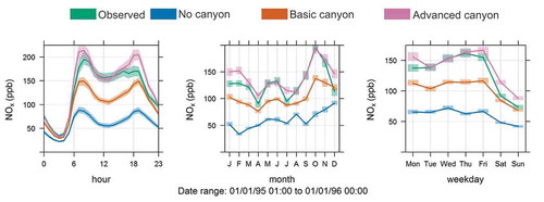
Figure 9. Wind rose (left) and Polar concentration NO₂ (µg/m³) plots for Marylebone Road. The polar concentration plots have wind speed on the radial axis, and wind direction on the azimuth angle, with four datasets: No canyon (top left), Basic canyon (top right), Advanced canyon (bottom left), and observations (bottom right). Combinations of wind direction and wind speed which occur for fewer than 5 hours in the year are grayed out in the concentration plots. Please refer to the online version for color figures

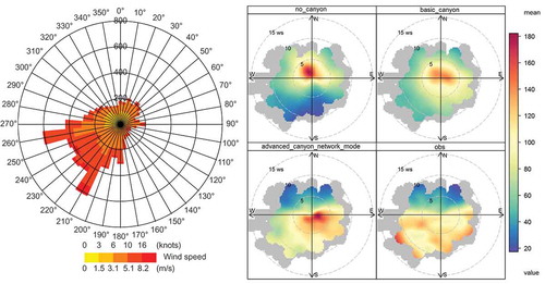
Figure 10. Comparison of modeled concentrations with and without the use of the ADMS-Urban urban canopy (UC) flow option for the no canyon, basic canyon and advanced canyon configurations: London 2012 dataset, with sites categorized according to Background, Near road (all) and Strong canyons

References

- Ahmad, K., M. Khare, and K. K. Chaudhry. 2005. Wind tunnel simulation studies on dispersion at urban street canyons and intersections—a review. J. Wind Eng. Ind. Aerod. 93 (9):697–717. doi:10.1016/j.jweia.2005.04.002.
- Azzi, M., and G. Johnson. 1992. An introduction to the generic reaction set photochemical smog mechanism. Proc. 11th Clean Air Conf. 4th Regional IUAPPA Conf., Brisbane, Australia, July.
- Beevers, S., D. Carslaw, E. Westmoreland, and H. Mittal. 2009. Air pollution and emissions trends in London. Report for Defra. Accessed July 1, 2020. https://uk-air.defra.gov.uk/assets/documents/reports/cat05/1004010934_MeasurementvsEmissionsTrends.pdf
- Benavides, J., M. Snyder, M. Guevara, A. Soret, C. P. García-Pando, F. Amato, X. Querol, and O. Jorba. 2019. CALIOPE-Urban v1.0: Coupling R-LINE with a mesoscale air quality modelling system for urban air quality forecasts over Barcelona city (Spain). Geosci. Model Dev. 12 (7):2811–35. doi:10.5194/gmd-12-2811-2019.
- Carslaw, D. C., and K. Ropkins. 2012. openair — An R package for air quality data analysis. Environ. Model. Softw. 27–28:52–61. doi:10.1016/j.envsoft.2011.09.008.
- CERC, 2017a. ADMS-Urban Technical Specification document P25/03J/17: Implementation of area, volume and line sources. accessed July 1, 2020. http://www.cerc.co.uk/environmental-software/assets/data/doc_techspec/P25_03.pdf.
- CERC. 2017b. ADMS-Urban Technical Specification document P28/01C/17: Basic street canyon model. Accessed July 1, 2020. http://www.cerc.co.uk/environmental-software/assets/data/doc_techspec/P28_01.pdf
- CERC. 2017c. ADMS-Urban Technical Specification document P34/01A/17: Urban canopy flow specification. Accessed July 1, 2020. http://www.cerc.co.uk/environmental-software/assets/data/doc_techspec/P34_01A.pdf
- CERC. 2020a. ADMS-Urban Technical Specification document P31/01C/20: Road sources. Accessed July 1, 2020. http://www.cerc.co.uk/environmental-software/assets/data/doc_techspec/P31_01.pdf
- CERC. 2020b. ADMS-Urban Technical Specification document P18/03E/20: Urban chemistry including the trajectory model. Accessed July 1, 2020. http://www.cerc.co.uk/environmental-software/assets/data/doc_techspec/P18_03.pdf
- Chang, J. C., and S. R. Hanna. 2004. Air quality model performance evaluation. Meteorol. Atmos. Phys. 87 (1–3):167–96. doi:10.1007/s00703-003-0070-7.
- Greater London Authority (GLA). 2013. London Atmospheric Emissions Inventory (LAEI) 2010. Accessed July 1, 2020. https://data.london.gov.uk/dataset/london-atmospheric-emissions-inventory-2010
- Green, D. 2002. Marylebone road (‘Supersite’) annual report 2000. King’s College London Environmental Research Group. Accessed July 1, 2020. https://uk-air.defra.gov.uk/library/reports?report_id=155
- Hertel, O., R. Berkowicz, and S. Larssen. 1990. The Operational Street Pollution Model (OSPM). 18th International meeting of NATO/CCMS on Air Pollution Modelling and its Application, Vancouver, Canada, 741–49. doi:10.1007/978-1-4615-3720-5_86
- Hood, C., D. Carruthers, M. Seaton, J. Stocker, and K. Johnson. 2014. Urban canopy flow field and advanced street canyon modelling in ADMS-Urban. Paper presented at 16th International Conference on Harmonisation within Atmospheric Dispersion Modelling for Regulatory Purposes, Varna, Bulgaria, September 2014. http://www.harmo.org/Conferences/Proceedings/_Varna/publishedSections/H16-067-Hood-EA.pdf.
- Hood, C., I. MacKenzie, J. Stocker, K. Johnson, D. Carruthers, M. Vieno, and R. Doherty. 2018. Air quality simulations for London using a coupled regional-to-local modelling system. Atmos. Chem. Phys. 18 (15):11221–45. doi:10.5194/acp-18-11221-2018.
- Hu, C.-B., F. Zhang, F.-Y. Gong, C. Ratti, and X. Li. 2020. Classification and mapping of urban canyon geometry using Google Street View images and deep multitask learning. Build. Environ. 167:106424. doi:10.1016/j.buildenv.2019.106424.
- Jackson, M., C. Hood, C. Johnson, and K. Johnson. 2016. Calculation of Urban Morphology Parameterisations for London for use with the ADMS-Urban Dispersion Model. Int. J. Adv. Remote Sens. GIS 5 (4):1678–87. doi:10.23953/cloud.ijarsg.52.
- Kakosimos, K., O. Hertel, M. Ketzel, and R. Berkowicz. 2010. Operational Street Pollution Model (OSPM) - A review of performed application and validation studies, and future prospects. Environ. Chem. 7 (6):485–503. doi:10.1071/EN10070.
- Keller, M., S. Hausberger, C. Matzer, P. Wüthrich, and B. Notter. 2017. HBEFA version 3.3. Background documentation, 12. Berne. Available online at https://www.hbefa.net/e/documents/HBEFA33_Documentation_20170425.pdf
- Kim, Y., Y. Wu, C. Seigneur, and Y. Roustan. 2018. Multi-scale modelling of urban air pollution: Development and application of a Street-in-Grid model (v1.0) by coupling MUNICH (v1.0) and Polair3D (v1.8.1). Geosci. Model Dev. 11 (2):611–29. doi:10.5194/gmd-11-611-2018.
- LAQN London Air Quality Network. 2017. Accessed July 1, 2020. https://www.londonair.org.uk/london/asp/publicdetails.asp
- Manning, A. J., K. J. Nicholson, D. R. Middleton, and S. C. Rafferty. 2000. Field study of wind and traffic to test a street canyon pollution model. Environ. Monit. Assess. 60 (3):283–313. doi:10.1023/A:1006187301966.
- Murena, F., G. Favale, S. Vardoulakis, and E. Solazzo. 2009. Modelling dispersion of traffic pollution in a deep street canyon: Application of CFD and operational models. Atmos. Environ. 43 (14):2303–11. doi:10.1016/j.atmosenv.2009.01.038.
- Oke, T. R. 1988. Street design and urban canopy layer climate. Energy Build. 11 (1–3):103–13. doi:10.1016/0378-7788(88)90026-6.
- Ordnance Survey MasterMap Integrated Transport Network Layer and Topography Layer (GML geospatial data). London: Coverage. Updated 18 December 2014. Ordnance Survey, GB. Using: EDINA Digimap Ordnance Survey Service. http://digimap.edina.ac.uk, Downloaded: May 2015.
- Owen, B., H. A. Edmunds, D. J. Carruthers, and R. J. Singles. 2000. Prediction of total oxides of nitrogen and nitrogen dioxide concentrations in a large urban area using a new generation urban scale dispersion model with integral chemistry model. Atmos. Environ. 34 (3):397–406. doi:10.1016/S1352-2310(99)00332-5.
- Ricardo-AEA. 2013. QA/QC data ratification report for the automatic urban and rural network, October-December 2012, and annual review 2012. Report for Department for Environment, Food and Rural Affairs, The Scottish Government, The Welsh Government, The Northern Ireland Department of Environment. Ricardo-AEA/R/3364 issue 1. Accessed July 1, 2020. https://uk-air.defra.gov.uk/assets/documents/reports/cat05/1307171010_QAQC_Ricardo_Q4_2012_Issue_1.pdf.
- Robins, A., and C. McHugh. 2001. Development and evaluation of the ADMS building effects module. Int. J. Environ. Pollut. 16 (1–6):161–74. doi:10.1504/IJEP.2001.000614.
- Snyder, M. G., A. Venkatram, D. K. Heist, S. G. Perry, W. B. Petersen, and V. Isakov. 2013. RLINE: A line source dispersion model for near-surface releases. Atmos. Environ. 77:748–56. doi:10.1016/j.atmosenv.2013.05.074.
- Soulhac, L., P. Salizzoni, F. X. Cierco, and R. Perkins. 2011. The model SIRANE for atmospheric urban pollutant dispersion; part I, presentation of the model. Atmos. Environ. 45 (39):7379–95. doi:10.1016/j.atmosenv.2011.07.008.
- Stidworthy, A., D. Carruthers, J. Stocker, D. Balis, E. Katragkou, and J. Kukkonen. 2013. Myair toolkit for model evaluation. 15th International Conference on Harmonisation within Atmospheric Dispersion Modelling for Regulatory Purposes, Madrid, Spain.
- Tominaga, Y., and T. Stathopoulos. 2013. CFD simulation of near-field pollutant dispersion in the urban environment: A review of current modeling techniques. Atmos. Environ. 79:716–30. doi:10.1016/j.atmosenv.2013.07.028.
- TRAPOS Optimisation of modelling methods for traffic pollution in streets. Accessed July 1, 2020. http://www2.dmu.dk/AtmosphericEnvironment/trapos.
- Vardoulakis, S., B. E. Fisher, K. Pericleous, and N. Gonzalez-Flesca. 2003. Modelling air quality in street canyons: A review. Atmos. Environ. 37 (2):155–82. doi:10.1016/S1352-2310(02)00857-9.
- Willmott, C. J., S. M. Robeson, and K. Matsuura. 2012. A refined index of model performance. Int. J. Climatol. 32 (13):2088–94. doi:10.1002/joc.2419.
- Yuan, C., E. Ng, and L. K. Norford. 2014. Improving air quality in high-density cities by understanding the relationship between air pollutant dispersion and urban morphologies. Build. Environ. 71:245–58. doi:10.1016/j.buildenv.2013.10.008.