Methane flux from flowback operations at a shale gas site

ABSTRACT

We report measurements of methane (CH₄) mixing ratios and emission fluxes derived from sampling at a monitoring station at an exploratory shale gas extraction facility in Lancashire, England. Elevated ambient CH₄ mixing ratios were recorded in January 2019 during a period of cold-venting associated with a nitrogen lift process at the facility. These processes are used to clear the well to stimulate flow of natural gas from the target shale. Estimates of CH₄ flux during the emission event were made using three independent modeling approaches: Gaussian plume dispersion (following both a simple Gaussian plume inversion and the US EPA OTM 33-A method), and a Lagrangian stochastic transport model (WindTrax). The three methods yielded an estimated peak CH₄ flux during January 2019 of approximately 70 g s⁻¹. The total mass of CH₄ emitted during the six-day venting period was calculated to be 2.9, 4.2 ± 1.4(1σ) and 7.1 ± 2.1(1σ) tonnes CH₄ using the simple Gaussian plume model, WindTrax, and OTM-33A methods, respectively. Whilst the flux approaches all agreed within 1σ uncertainty, an estimate of 4.2 (± 1.4) tonnes CH₄ represents the most confident assessment due to the explicit modeling of advection and meteorological stability permitted using the WindTrax model. This mass is consistent with fluxes calculated by the Environment Agency (in the range 2.7 to 6.8 tonnes CH₄), using emission data provided by the shale site operator to the regulator. This study provides the first CH₄ emission estimate for a nitrogen lift process and the first-reported flux monitoring of a UK shale gas site, and contributes to the evaluation of the environmental impacts of shale gas operations worldwide. This study also provides forward guidance on future monitoring applications and flux calculation in transient emission events.

Implications: This manuscript discusses atmospheric measurements near to the UK’s first hydraulic fracturing facility, which has very high UK public, media, and policy interest. The focus of this manuscript is on a single week of data in which a large venting event at the shale gas site saw emissions of ~4 tonnes of methane to atmosphere, in breach of environmental permits. These results are likely to beresults are likely to be reported by the media and may influence future policy decisions concerning the UK hydraulic fracturing industry.

Introduction

Energy production through the combustion of fossil fuels is associated with the emission of greenhouse gases. The burning of natural gas, which largely comprises methane (CH₄), directly produces carbon dioxide (CO₂). Hydraulic fracturing (colloquially referred to as “fracking”) of shale gas formations for the extraction of natural gas has gained wide-spread attention in the past decade. Energy derived from the hydraulic fracturing processes has been proposed as a “cleaner” alternative to the carbon-intensive combustion of coal in the UK energy sector. However, this assumption depends on the proportion of CH₄, a prominent greenhouse gas, released to the atmosphere through intentional venting, accidental leakage (fugitive emissions) or as a non-combusted component of flaring.

A recent study proposed that the rapid growth in unconventional shale gas production in North America may account for a large proportion of the observed increases in global CH₄ levels since 2007 (Howarth 2019). However, this finding is contended; the global decrease in CH₄ carbon isotope ratio (δ¹³C_CH₄) since 2007 is not accounted for by the isotopic ratio of the majority of shale gas emissions (Milkov et al. 2020). Many other studies attribute the rapid rise in CH₄ to an increase in the extent and productivity of biogenic CH₄ sources (such as wetlands; Nisbet et al. 2016), changes in global CH₄ sinks (Rigby et al. 2017; Turner et al. 2017) or changes in global biomass burning (Hausmann, Sussmann, and Smale 2016; Schaefer et al. 2016; Worden et al. 2017) with some studies suggesting fossil fuel emissions have actually been stable since 2008 (Schwietzke et al. 2016).

In recent years, various life cycle assessment (LCA) studies have attempted to estimate the overall carbon footprint of unconventional gas as an energy source. The majority of these studies have occurred in the USA due to its well-established industry. Studies for other countries, such as the UK, lack their own domestic operational data and often rely partly on extrapolated data from US analogues. These studies have estimated the mean carbon footprint of shale gas at approximately 67 g CO_2-equivalents (CO₂e) MJ⁻¹, but a range of life cycle assumptions have yielded estimates in the range 56 to161 g CO₂e MJ⁻¹ (Cooper, Stamford, and Azapagic 2014; MacKay and Stone 2013; Stamford and Azapagic 2012; Weber and Clavin 2012). Whilst most studies have highlighted the importance of a well’s estimated ultimate recovery (EUR) in determining the carbon footprint, intentional and unintentional CH₄ emissions have been singled out as a key source of uncertainty. Emissions of CH₄ vary from 0% to 7.9% of the EUR, with typical estimates of approximately 0.1% to 0.2% for the likely range of UK well’s EUR (Cooper, Stamford, and Azapagic 2014; MacKay and Stone 2013; Stamford and Azapagic 2012; Weber and Clavin 2012). The contribution of episodic events, including flowback and well unloading, to the overall carbon footprint of shale gas is thought to be significant (Allen et al. 2013). Moreover, the assumptions and uncertainties associated with these events constitute a primary source of discrepancy between bottom-up and top-down emission inventories (Vaughn et al. 2018). Short-term events are rarely studied and relatively few measurement examples exist in the literature (Allen et al. 2015, 2013; Rich, Grover, and Sattler 2014; Williams et al. 2018). However, such events must be included in carbon assessments to gain a more accurate understanding of total emissions from the oil and gas industry.

A nitrogen lift is a standard “artificial lifting” technique employed by both the onshore and offshore oil and gas industry to unload unwanted fluid in a well and to promote the flow of gas or oil from the hydrocarbon reservoir (EPA 2014; Gu 1995). The process involves pumping nitrogen gas to the base of the well, which lifts accumulated fluids (such as produced water and other well fluids) from the borehole as it returns to the surface. Nitrogen lifts, or other enhanced recovery well operations, are not typically required following high volume hydraulic fracturing of shales. A shale gas well that has been stimulated in line with its design will normally have a very large initial flow of well gas that lifts any fracturing fluids and naturally occurring liquids to the surface unaided.

The prospective and exploratory phases of nascent unconventional gas extraction are poorly quantified in existing literature. LCA typically models commercial-scale processes under normal operating conditions and therefore includes well construction but may exclude any prior phases of testing and exploration that do not lead directly to commercial operation. This is true of conventional, as well as unconventional, fossil fuel life cycles. For example, in Ecoinvent – the most widespread LCA database, particularly in Europe – the only dataset describing onshore natural gas exploration is the same as that for commercial well construction and is based on data from Nigeria, India, and various multinational companies in the late 1990s (Ecoinvent 2018). Consequently, the UK is uniquely placed to gather important new data by observing these early stages of the industry to address this knowledge gap. This has been demonstrated in Lowry et al. (2020), Purvis et al. (2019) and Shaw et al. (2019), in which local climatological baselines of greenhouse gases and air quality components were defined at two UK sites proposed for hydraulic fracturing shale gas development. Further, Shaw et al. (2019) developed a statistically derived algorithm for quick detection of CH₄ enhancements (such as emission events) based on exceedances of the baseline conditions.

In this study, we provide an analysis of the CH₄ enhancements measured from a fixed-site monitoring station adjacent to the UK’s only operating onshore shale gas facility to use hydraulic fracturing, at the time of writing. We provide estimates of CH₄ fluxes and the CH₄ mass vented to the atmosphere during these operations with the aim of comparing against both operator and regulator reported values. We also assess different flux quantification methods for their applicability to deriving fluxes from fixed-site monitoring of facility scale emissions for future monitoring applications. The climate relevance of the CH₄ emissions is also briefly discussed, in the context of the UK Government’s net-zero carbon ambitions, through analysis of CO₂-equivalents and GWP. Whilst this manuscript focuses on emissions of greenhouse gases from the shale gas facility during well unloading, simultaneous emissions of gases important for air quality were also observed and will be reported in future work.

Monitoring site design

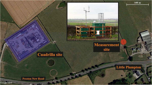
The location of the fixed-site monitoring station relative to the Cuadrilla Resources Ltd shale gas extraction facility in Little Plumpton, Lancashire is shown in Figure 1. The measurement station is located on a privately owned farm approximately 430 m to the east of the Cuadrilla facility and 100 m north of Preston New Road (PNR). The measurement site was located downwind (to the east), in the dominant prevailing wind direction (westerly), of the shale gas infrastructure to optimize the likelihood of sampling emissions associated with operational activity. A high-precision in situ CO₂ and CH₄ mixing ratio analyzer (Ultra-portable Greenhouse Gas Analyzer (UGGA); Los Gatos Research Inc., USA) has been recording data at the measurement site since January 2016. Equipment for the measurement of meteorological conditions was also installed, alongside instrumentation for the sampling of atmospheric components important for air quality assessment (see Supplementary Information Table S1 and Purvis et al. (2019) for more information).

Figure 1. Google Maps © image (dated 26 September 2018) of the Cuadrilla Resources Ltd owned onshore shale gas extraction facility (blue square) and the nearby monitoring station (red circle). The measurement site is approximately 430 m to the east of the Cuadrilla site boundary and 100 m north of Preston New Road. There is a gradual 12 m increase in elevation from the Cuadrilla site to the measurement station. The buildings 100 m to the east of the measurement site are part of a dairy and cattle farm. Cattle make use of the surrounding fields throughout the summer period but were not present in the field between the shale gas site and the measurement site in January 2019. Other potential sources of pollution include: leaks from natural gas infrastructure on Preston New Road, a motorway (M55; 1.3 km to the north), and a landfill site (2.6 km to the south west) (see Lowry et al. 2020 for more details)

The UGGA instrument was calibrated in the field using gas standards traceable through an unbroken chain to World Meteorological Organization (WMO) international standards (X2007 for CO₂ and X2004A for CH₄). Calibrations were performed during regular site maintenance visits (roughly every 3 weeks), using gas from three 40 L laboratory standards (filled by Deuste, Steininger GmbH, Germany, and certified on the WMO scale by EMPA, Switzerland) decanted into 6 L SilcoCan canister (Thames Restek, UK) for transport. Further detail on the calibration procedures and quality assurance measures used to ensure data quality can be found in Shaw et al. (2019). Data from the UGGA instruments were corrected for small systematic errors associated with water vapor using the procedure outlined by O’Shea et al. (2013). The 1-min average CH₄ and CO₂ data have 95% confidence intervals of approximately 5–10 ppb and 0.5–0.8 ppm, respectively. Calibrated and quality-assured datasets from the baseline project are publicly available on the Center for Environmental Data Analysis Archive (CEDA Archive; http://www.ceda.ac.uk/; Purvis 2019).

Exploratory shale gas extraction using hydraulic fracturing began at PNR in October 2018 with flowback commencing in November 2018 following partial fracturing of the well. Commercial production of natural gas at PNR had not yet started. Prior to operational activity, a two-year monitoring program administered by the British Geological Survey, and conducted by the University of Manchester, Royal Holloway University of London and the National Center for Atmospheric Science (NCAS; based at the University of York), was tasked to define a local baseline climatology of ambient mixing ratios of pollutants. These baseline climatologies have been reported for atmospheric greenhouse gases (Lowry et al. 2020; Shaw et al. 2019) and for air quality (Purvis et al. 2019) and contextualize preexisting atmospheric conditions for use as a control against which the incremental impacts of new industrial activities can be assessed. This work also identified and characterized local sources of greenhouse gases, which may influence the CH₄ measurements at the monitoring site. Such sources (within 2 km of the PNR) are described in Lowry et al. (2020). The dairy farm and its surrounding grazing land (with approximately 250 cattle), on which the monitoring station is located, was identified as a major source of atmospheric CH₄. To this end, a set of threshold criteria were developed to quickly interpret excursions (such as CH₄ emission events) based on the statistical set of baseline conditions. These criteria (described in detail in Shaw et al. 2019), select for periods in which exceedances of the 99th percentile of CH₄ mixing ratio coincide with westerly winds (270° ± 45°), wind speeds greater than 2 m s⁻¹ and low-to-no enhancements in CO₂ mixing ratios. These thresholds were used to automatically flag periods of CH₄ enhancement in this study.

Flux estimation methods

The site operator confirmed that nitrogen lift operations, undertaken to promote flowback after partial hydraulic fracturing of the well, resulted in the controlled venting of unflared CH₄ between 11 and 16 January 2019. The mixture of natural gas and nitrogen was noncombustible and the flare failed to light, leading to direct venting of natural gas to the atmosphere. During this time, the operators reported peak natural gas (>95% CH₄) flow rates of 200,000 cubic feet per day (equivalent to approximately 44 g s⁻¹ CH₄ at surface pressure and 15°C) and stable flow of 100,000 cubic feet per day (equivalent to approximately 22 g s⁻¹ CH₄) (see Cuadrilla Resources Ltd 2019). Calculations, made by the Environment Agency (using operator provided data), estimated that “between 2.7 and 6.8 tonnes of CH₄ was vented [to the atmosphere]” during this time (Environment Agency 2019a), where these two values reflect the choice of assumed global warming potential (GWP) time horizon (20 or 100 years) (see Section 4.2).

The three different methods described below were used to estimate CH₄ fluxes during the emission event in January 2019 using data from the fixed-site monitoring station to compare against the operator and regulator reported values. The chosen flux estimation methodologies are commonly used by researchers but are also routinely employed by industry for air monitoring purposes, and the methodologies are consistent with regulatory standards in North America (US EPA 2014).

All flux quantification methods employed here required the use of a CH₄ background value to determine the CH₄ enhancement. The 0.1^th percentile of CH₄ mixing ratios measured during January in the baseline period (2017 and 2018) under westerly winds, equivalent to 1.91 ppm CH₄, was used as the CH₄ background value (see Shaw et al. 2019, or Table S3 in the Supplementary Information). However, the dynamic nature of the ambient CH₄ measured at PNR during the baseline period, which varied considerably with wind direction, time-of-day, and season, meant that the choice of a single background value is subjective. For this reason, the three methods were tested for their sensitivity toward a range of CH₄ background values, between 1.86 and 1.95 ppm CH₄. These CH₄ background values were in broad agreement with CH₄ mixing ratios, of approximately 1.92 ppm CH₄, measured at the Mace Head Global Atmospheric Watch (GAW) station during the enhancement period (Prinn et al. 2020).

Simple Gaussian dispersion

Estimates of the CH₄ flux during the emissions period (11–16 January) were made using a simple Gaussian plume dispersion model (Connolly 2019). The simulations were modeled for a monitoring station characteristic of that at PNR; i.e. 430 m downwind in the prevailing wind direction (and therefore in the center of the plume) from flare stacks at the site. The flare stacks were assumed to be a point source of emission. Three Pasquill atmospheric stability classes (classes C, D, and E, equivalent to “slightly stable,” “neutral,” and “slightly unstable”) were used for the simulations to provide an indication of the sensitivity of the analysis to atmospheric turbulence, and to provide a rough estimate of flux uncertainty (Pasquill 1961). The dispersion parameters used in the Gaussian function were taken from the rural mode of the Pasquill-Gilford formulae (Turner 1970).

US EPA OTM-33

Flux was also estimated using a point-source Gaussian (PSG) flux estimation model adapted from that described in OTM-33A (US EPA 2014). OTM-33 provides a set of United States Environmental Protection Agency (EPA) standardized methods for the geospatial measurement of air pollution, remote emissions quantification, and direct assessment. The method is usually applied to measurements made using mobile monitoring within 200 m of the source but can be used for stationary measurement approaches (e.g. Foster-Wittig, Thoma, and Albertson 2015). PSG is an emission quantification method suited for single-point stationary observations and uses a Gaussian approximation and dispersion lookup tables. The OTM-33 methods are described further on the EPA website (https://www.epa.gov/emc). Previous assessments of the OTM method, using controlled releases of CH₄, concluded a typical 1σ uncertainty in flux estimation in the range of ± 30% (Brantley et al. 2014; Robertson et al. 2017; Saide et al. 2018).

Stochastic Lagrangian inversion

CH₄ flux was also estimated using the WindTrax 2.0 Model (ThunderBeach Scientific, www.thunderbeachscientific.com). WindTrax is a Lagrangian stochastic (LS) particle model for the assessment of atmospheric transport of pollutants over small horizontal distances (less than 1 km; Flesch et al. 2009; Flesch, Wilson, and Yee 1995). A CH₄ emission strength (from a point source) was estimated using measured 15-min average CH₄ mixing ratios and a wind field calculated from 15-min average 3-dimensional wind measurements during the period 11 January to 16 January 2019. The CH₄ source strength was estimated by computing the advection of 150,000 particles from the flare stacks to the detector in forward LS mode. The simulation used an assumption that the surface layer consisted entirely of short grass, with a surface roughness length (Z_o) of 2.3 cm. The use of WindTrax is also included in OTM-33 and it has been used previously to estimate CH₄ emission fluxes from disperse sources such as landfill sites (e.g. Riddick et al. 2017).

A second set of WindTrax simulations were also performed in this study for the period 1 February 2018 to 31 January 2019 to derive a contextually comparative CH₄ flux from a nearby dairy farm (simulated as a diffuse area source) to the east of the monitoring station. These simulations used measured 15-min average CH₄ mixing ratios and a wind field calculated from 15-min average two-dimensional meteorological parameters. The CH₄ background mixing ratio was derived monthly to account for seasonality in CH₄ mixing ratios. Except for the particle count, which was reduced to 50,000 for the dairy farm assessment, all other parameters were identical to those above.

Results and discussion

The “baseline period” refers to measurements made between 1 February 2016 and 31 January 2018. The “emissions period” refers to measurements made between 10 January 2019 and 16 January 2019.

Fixed-station CH₄ measurements

Exploratory hydraulic fracturing operations commenced at PNR in mid-October 2018 with flowback beginning in November 2018 following partial fracturing of the well. Enhancements in CH₄ mixing ratios potentially related to this activity were first observed on 7^th December during a short period of westerly winds passing over the site toward the monitoring station. The wind direction was unfavorable for further detection of emissions during December 2018. Favorable wind conditions for observational monitoring returned in January 2019, along with clear enhancements in CH₄ mixing ratios relative to the baseline. It is unlikely that the enhanced CH₄ posed any explosive or health risk to the workforce, or to the local population. However, the observed CH₄ enhancements were correlated with elevated mixing ratios of other atmospheric components, such as NO_x and volatile organic compounds. Whilst NO_x mixing ratios did not exceed EU 1-hr average threshold criteria, such emissions have the potential to photochemically produce ozone (Cooper, Stamford, and Azapagic 2014). These measurements, and their potential health and environmental impacts, will be discussed in future work.

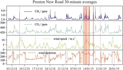
Figure 2 shows 30 min averaged CH₄ and CO₂ mixing ratios measured at PNR for the period 1 December 2018 through to 31 January 2019. Greenhouse gas mixing ratios are shown alongside wind speed and wind direction to illustrate meteorological conditions during the period. The predominance of westerly winds between 11 and 16 January meant that major local CH₄ sources, such as the dairy farm and landfill site, had little influence on the CH₄ measurements made at the monitoring station. The areas highlighted in red represent hourly periods in which CH₄ exceeded the baseline threshold criteria of Shaw et al. (2019). A number of clear excursions in CH₄ mixing ratio occurred in January, concurrent with relatively high westerly wind speeds, but with no associated enhancement in CO₂ mixing ratio. This is consistent with cold-vented (non-flared) emissions of natural gas.

Figure 2. Thirty-minute averaged CH₄ and CO₂ mixing ratios, wind speeds, and wind direction at the PNR monitoring station for the period 1 December 2018 to 31 January 2019. The red highlighted areas represent hourly periods which exceeded the threshold criteria for the identification of excursions from the baseline conditions (Shaw et al. 2019)

No notable enhancements in CH₄ were recorded at the measurement station on 15 January 2019 but enhancements were observed on adjacent days, reflecting the dynamic nature of the emission flux. It was not possible to determine whether the absence of measured enhancements on that day was due to a subtle change in wind direction, or due to there simply being no emissions. This highlights a key limitation of single fixed-site measurements; had the wind direction been different during the event (e.g. from the east), the CH₄ emission would not have been observed. It is therefore difficult to make an assessment of the total amount of time that CH₄ was emitted from the shale gas site during any periods of unfavorable wind direction. Any flux estimates should therefore be interpreted with this in mind as they may represent an underestimate as a result of missed emissions. A future solution to this dependency on favorable wind direction would be to install multiple monitoring stations around the site of interest, but this is typically cost-prohibitive for high-precision instruments such as those used here. Alternatively, a rapid-response mobile survey, such as unmanned aerial vehicle (UAV) or vehicle monitoring could be deployed to sample downwind of the shale gas facility. However, this is logistically challenging and relies on prior warning of emissions, which may not always be given. Other solutions could involve cheaper sensor networks but with the caveat of inherently reduced flux precision if low precision instruments are used.

CH₄ flux results

Simple Gaussian plume simulations resulted in an estimated peak CH₄ flux of 138 (± 60) g s⁻¹ for the emission period when using stability class C (Table 1). Integrating the calculated flux values over time resulted in three estimates for the total CH₄ mass emitted; these were 2.9 (± 1.3), 1.3 (± 0.6) and 0.9 (± 0.4) tonnes CH₄ for stability classes C, D, and E, respectively. The fluxes and mass estimates calculated using this Gaussian plume model were likely to be uncertain due to the use of generic stability classes (and not measured meteorological data). This is discussed further in Section 4.2.1.

Table 1. Peak CH₄ fluxes and total CH₄ mass emitted during the emissions period (11–16 January) simulated using Gaussian plume modeling (Connolly 2019)

Stability class	C (slightly unstable)	D (neutral)	E (slightly stable)
Peak CH4 flux/g s^−1	138 ± 60	63 ± 27	44 ± 19
CH4 mass emitted/tonnes	2.9 ± 1.3	1.3 ± 0.6	0.9 ± 0.4

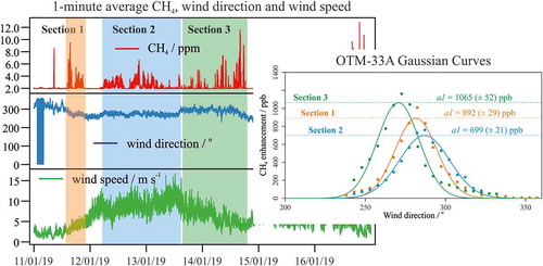
Analysis using the OTM-33A PSG method provided a CH₄ flux estimate for each of three time periods (based on consistent wind direction; see Figure 3). Some of the parameters calculated during application of this method are outlined in Table 2. In the absence of intrinsic uncertainty propagation within this method, a 1σ uncertainty of ± 30% (as suggested by Saide et al. (2018)) was applied to each of the calculated fluxes. The CH₄ flux values calculated using OTM-33 for each of these time periods were in good agreement with the peak CH₄ flux estimated by the Gaussian plume model with stability class D. Emitted CH₄ mass estimates were calculated by multiplying the estimated CH₄ flux by the number of hours where baseline thresholds were exceeded for each time period. These estimates rely on an assumption that the source emission rate was constant throughout each time period. The total CH₄ mass emitted for the six-day period in January 2019, as estimated by OTM-33A, was 7.1 (± 2.1) tonnes. This is in agreement with the upper value of the Environment Agency estimate (6.8 tonnes CH₄).

Table 2. OTM-33A parameters for three different time periods (see Figure 3) during the January event

	Section 1	Section 2	Section 3
Start time (UTC)	11/01/19 12:00	12/01/19 03:00	13/01/19 16:00
End time (UTC)	11/01/19 23:00	13/01/19 16:00	14/01/19 19:00
Estimated peak CH4/ppb	892 ± 29	699 ± 21	1065 ± 52
σy/m	90.88	63.17	76.42
σz/m	51.99	36.17	42.75
Wind speed/m s^−1	3.3 ± 1.3	8.3 ± 2.1	4.2 ± 1.5
Calculated CH4 flux/g s^−1	58 ± 17	56 ± 17	64 ± 19
CH4 mass emitted/tonnes	1.2 ± 0.4	3.6 ± 1.1	2.3 ± 0.7

Figure 3. One-minute average CH₄ mixing ratio and wind direction at PNR in January 2019. The plot shows the three sections chosen for analysis by OTM-33A. Each section corresponds roughly to CH₄ enhancements observed during a period of consistent wind direction. The plot on the right shows the Gaussian approximations for each of the three sections, with CH₄ enhancement over background averaged into 5 degree wind direction bins. The Gaussian approximations are shown by the continuous lines, with the maximum value for each Gaussian curve (a1) shown by the dashed lines

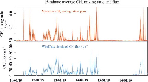
Figure 4 shows the WindTrax-simulated 15-min average CH₄ flux as a function of time for the emissions period. A maximum flux, equal to 81 (± 68) g s⁻¹ was simulated at 21:00 on 16 January. The mean flux throughout the period was 16.3 g s⁻¹. Multiplying the instantaneous flux in each model time step period (15 min) and summing over the whole period provides an estimate of the total CH₄ vented to the atmosphere of 4.2 (± 1.4) tonnes CH₄. This is in agreement with the Environment Agency estimate (2.7 and 6.8 tonnes CH₄) and overlaps well (within 1σ uncertainty) with the estimate made using the OTM-33A method.

Figure 4. Fifteen-minute average measured CH₄ mixing ratio and WindTrax-simulated CH₄ flux for the enhancement period. The transparent colored areas show the standard deviation (1σ) in CH₄ mixing ratio and flux

It is important to note that the two estimates of total vented CH₄ reported by the Environment Agency (see Environmental Agency, 2019a) were calculated from an operator-provided estimated emission of 230 tonnes CO₂-equivalent. This was converted to two CH₄ masses using global warming potential (GWP) values with different GWP time horizons (Environment Agency 2019b; see Myhre et al. (2013) for GWP values and further information on the conversion to CO₂-equivalent mass). The Environment Agency Compliance Assessment (Environment Agency 2019a) reported the total CH₄ emitted as a range between 2.7 and 6.8 tonnes. However, we note that it may have been incorrect to describe this as a range, as in principle it should be one mass or the other, depending on the explicit GWP time horizon used to initially convert the vented CH₄ to CO₂-equivalent mass. To avoid such misunderstanding in future, we recommend that a consistent GWP time horizon is used to convert between CH₄ mass and CO₂-equivalent mass, and that a single flux value (and GWP time horizon) is publicly reported to avoid unnecessary confusion.

WindTrax simulations for the period 1 February 2018 to 31 January 2019 were also used to estimate CH₄ fluxes from the dairy farm to the east of the monitoring station for a contextual comparison. CH₄ fluxes were calculated throughout the year, with a mean flux of 1.5 (± 3.9) g s⁻¹ interspersed with short periods in which fluxes approached 100 g s⁻¹. The total CH₄ mass emitted from the dairy farm over the 12-month period was estimated to be 76 (± 175) tonnes CH₄, when proportionally extrapolated for periods in which winds were not favorable for sampling of dairy farm emissions. We provide this estimate here to offer some context and comparison with the shale gas site, whilst noting that the corresponding uncertainties are larger than the derived emissions themselves, and that there may have been some influence from the gas supply leaks identified by Lowry et al. (2020) (see Supplementary Information Section 2 and Fig. S2).

A summary of the results from the three flux estimate methods is presented in Table 3, alongside the operator/regulator reported values and flux estimates from mobile UAV surveys. The peak flux reported for the simple Gaussian plume simulation was time averaged to 15 min to match the WindTrax time-step interval. The peak flux values for each of the three methods were all in agreement with each other and with the operator reported peak gas flow, within 1σ uncertainty. These values were also in excellent agreement with fluxes calculated from four UAV surveys, which reported instantaneous emission fluxes within a range of 9 to 156 g s⁻¹ on 14 January (Shah et al. 2020a). The total CH₄ mass estimates were also in good agreement with each other, within their respective uncertainties (at 1σ). The range in which the three methods overlapped (2.9– 7.1 tonnes CH₄) represents the most likely confidence range of total CH₄ mass emitted. Unfortunately, there is no simple metric for determining which flux quantification method is the most accurate. The use of three different methods provides a useful comparison for their applicability to quantifying a CH₄ flux using long-term, continuous data from a fixed measurement site. In the authors’ opinions, the WindTrax estimated value of 4.2 (± 1.4) tonnes CH₄ represents the optimal assessment of cumulative emission from the nitrogen lift event, due to the model’s more explicit treatment of meteorology. We reiterate that there may have been a period of emission sampling dead-time (in which emissions were missed due to unfavorable wind direction), which none of these methods can account for, and that these values may therefore be an underestimate. However, the agreement with the CH₄ mass reported by the Environment Agency, which is based on emission data provided by the shale gas site operator, and the absence of enhancements observed during mobile vehicle surveys (see Supplementary Information Sections 3 and 4, and Figs. S4 and S5), suggests that the sampling dead-time may indeed have been a period of emission quiescence within the six-day event.

Table 3. Summary of peak and mean CH₄ fluxes, and total CH₄ mass emitted, as calculated by three different flux estimation methods. UAV measured fluxes derived from mobile surveys are also provided (see Shah et al. 2020a for more information) alongside the operator/regulator reported flux and total CH₄ mass estimates

Flux estimation method	Peak CH4 flux/g s^−1	Mean CH4 flux/g s^−1	Total CH4 mass emitted/tonnes
Simple Gaussian simulation^a	72 ± 31	5.6	2.9 ± 1.3
OTM-33A	64 ± 19	N/A	7.1 ± 2.1
WindTrax	81 ± 68	16.3	4.2 ± 1.4
UAV^b	9–156		N/A
Operator/regulator reported	44^c	22^c	2.7 or 6.8^d

Notes. ^aUsing stability class C and time-averaged to 15 min (to match the WindTrax iteration step).

^bShah et al. (2020a); reported as an instantaneous flux uncertainty range i.e. not time-averaged

^cCuadrilla Resources Ltd (2019)

^dEnvironment Agency (2019a)

Evaluation of flux methods and forward guidance

A critical evaluation of the flux approaches is made to guide those interested in attempting emissions calculations for transient events from large point sources. Such evaluation is highly important in greenhouse gas emissions science and policy, yet remains a practical and technical challenge.

The Gaussian plume simulation provided a flux under a range of possible meteorological stability scenarios. Figure S3 shows a time series comparison of WindTrax-simulated CH₄ flux and the simple Gaussian plume model simulated flux using stability class C (time averaged to match the WindTrax interval step of 15 min). The structure and features of the two time series were in good agreement throughout the emission period, despite there being a factor two difference in the estimate of total CH₄ mass emitted. This model showed only a small sensitivity to differences in the background CH₄ mixing ratio, up to at least 1.95 ppm. The use of a single stability class throughout the entire emissions period was unlikely to capture the true variation in atmospheric stability and thus represents a substantial limitation in the treatment of meteorology for this method. However, we recommend this method for quick and simple flux quantification, but note that the results must be interpreted without explicit meteorological context due to the use of generic and constant stability classes.

The OTM-33A method (applied to a stationary site) estimated flux using the Gaussian distribution of CH₄ enhancements as a function of wind direction. In principle, this method can work well for a fixed emitter with a constant flux rate but is less applicable to a source with varying strength, where variability in the actual source flux may be masked by any variability in wind direction. The OTM-33A method involves the estimation of a peak CH₄ mixing ratio using a Gaussian distribution function of CH₄ mixing ratios averaged within wind direction bins (Figure 3). The use of time-averaging and choice of bin width may also bias this calculation. Binning the CH₄ mixing ratios by wind direction results in averages which are affected by both the variability in flux strength and the variability in wind direction. These values were therefore unlikely to be truly representative of a mean (or a peak) mixing ratio in each 5° wind direction bin. Conceptually, this could be avoided by applying the method over shorter time periods in which the flux was likely to be more constant, and then integrating to obtain a total flux. However, when attempted here, this did not yield a large enough sample of data, especially of wind directions, to generate a meaningful Gaussian fit. The Draft EPA Method OTM-33A usually relies on mobile vehicle monitoring to sample CH₄ as a function of wind direction to either side of a plume. We conclude that the OTM-33A method is best suited to sources with a constant emission rate and may be subject to systematic error for dynamic sources. Additionally, the method relies on the subtraction of a background CH₄ mixing ratio to yield CH₄ enhancement. The resulting Gaussian distribution function was found to be sensitive to the choice of background CH₄ mixing ratio. The OTM-33A method includes a process for calculating the background mixing ratio but this may not be appropriate given the dataset, which requires manual inspection to ensure validity. Using different values for CH₄ background (from 1.91 to 1.95 ppm CH₄) resulted in discrepancies in calculated flux (from 55 to 76 g s⁻¹) and total CH₄ mass estimates (from 7.1 to 7.6 tonnes CH₄). Finally, the calculation of a total CH₄ mass during the emissions period was not trivial; simply multiplying the estimated flux by the number of enhanced hours of CH₄ relied on an assumption that the source strength was constant throughout that period. This is unlikely to be true for many industrial emission sources.

In our opinion, WindTrax provided the most comprehensive and meaningful flux analysis as it took account of measured meteorology (3D wind, temperature and pressure measurements) and used short model timesteps (15 min), which implicitly accounted for a dynamic CH₄ flux. However, like all other methods, WindTrax was sensitive to the mixing ratio used for CH₄ background with a factor of 1.6 difference in the estimated total mass of CH₄ emitted during the period when using different background values (from 1.91 to 1.95 ppm CH₄). Also, the WindTrax model could not explicitly account for surface topography from the emission point source to the measurement location (although it should be noted that this limitation also applied to the other two flux quantification methods as well). Two simulations were performed to investigate the sensitivity to this limitation: one in which the heights of the source and sensor were relative to the ground, and another in which the source and sensor heights were relative to each other. Table S2 outlines these results from WindTrax simulations. WindTrax was unable to resolve as many flux data points (i.e. model time steps) during the simulation with heights set relative to the ground. The model was also sensitive to the number of particles used during simulations; the smaller the particle count, the fewer flux values were resolved. We recommend that a model time step of 15 min, using 150,000 particles, and source and sensor positions relative to each other, are configured for any future flux assessment using WindTrax.

Climate change relevance

This study provides an estimated 4.2 (± 1.4) tonnes CH₄ emitted in only 6 days at the PNR shale gas site. Based on a typical lifespan of a shale gas operation of 10–30 years, one would expect the same mass of CH₄ to result from fugitive emissions from the steady state production of approximately 1.9 Mm³ shale gas, or 4–11 months’ worth of commercial extraction (Hultman et al. 2011; Jiang et al. 2011; Weber and Clavin 2012). This estimate aligns with field reports from the Montney shale gas development in north-western Canada (Atherton et al. 2017; Robinson et al. 2019) where annual wellsite-level emissions (fugitive and vents) during steady state production of shale gas amounts to 7.3 to 8.2 tonnes CH₄ per year per site on average.

Using the IPCC characterization factors (Myhre et al. 2013), 4.2 tonnes CH₄ equates to 143 tonnes CO₂-equivalents under the default 100-year time horizon (GWP100), or 361 tonnes CO₂-equivalents using a 20-year horizon (GWP20). The GWP100 value is equivalent to the carbon footprint of 516 MWh of electricity consumed from the UK National Grid (BEIS 2019): the annual electricity demand of 166 households (Ofgem 2019). Alternatively, equivalence can be drawn with 142 London–New York flights (BEIS 2019).

The relevance of these CH₄ flux estimates to LCA and carbon footprinting research is three-fold: firstly, data on emissions from the exploratory phases of gas extraction are only sparsely available and are not typically accounted for in LCA; secondly, to the best of the authors’ knowledge, existing literature does not account explicitly for nitrogen lift operations in gas extraction processes, making this the first available estimate; and thirdly, these data are some of the first emissions estimates for UK-specific shale gas operations, helping to lay the foundations for future life cycle assessment in this area.

Assuming the emission flux estimated in this work is representative of a typical flux from a nitrogen lift, the emitted CH₄ mass could conceivably be linearly extrapolated for a scaled-up hydraulic fracturing industry in the UK. This would allow for a simple assessment as to the importance of these transient events in the context of the UK greenhouse gas emissions inventory, which may be especially important given the UK government’s commitment to achieving net zero carbon emissions by 2050. However, such a linear extrapolation is difficult to achieve in practice for a number of reasons. Firstly, it is currently unknown whether this single emission event is truly representative of typical emissions from nitrogen lift, or other well-unloading, processes. Recently fractured wells rarely require artificial lifting techniques to stimulate flow and this likely only occurred due to partial completion of hydraulic fracturing. The emitted CH₄ mass reported here resulted from the cold-venting of CH_4, owing to a failure of the flare – successful flaring would have resulted in a decrease in the total mass of CH₄ vented to the atmosphere. Hence, reliably extrapolating this single measurement may introduce systematic bias. Secondly, it is not easy to reliably predict the potential extent of a UK-based onshore shale gas and hydraulic fracturing industry. Clancy et al. (2018) and the UK Onshore Oil and Gas organization predicted that there would be between 3,000 and 4,000 wells in a commercial UK onshore industry (UKOOG, 2019). However, this is currently far from certain given the moratorium on the use of hydraulic fracturing announced by the UK Government in November 2019. Finally, the frequency at which unloading processes are used to stimulate a well is highly variable; Allen et al. (2013) reported that some wells are unloaded monthly, and some only once per lifetime. Skone (2011) reported that, for 35,400 unconventional wells in the USA, there were 4,180 well-unloadings in 2007, suggesting wells are unloaded approximately once per decade. Robust measures for the reporting of such processes would need to be in place in order to make a comprehensive assessment of their impact in a future UK industry. Hence, extrapolating the measured CH₄ emission from this work to a scaled up industry should be considered as only a very rudimentary assessment, with potentially large uncertainties and systematic biases.

The nitrogen lift yielded a sustained CH₄ emission as part of flowback operations following partial hydraulic fracturing of the PNR well. It is possible to capture flowback emissions using specialized infrastructure in a process called Reduced Emission Completion (REC). RECs are being considered by the UK Government as part of a regulatory structure for shale gas. Whether nitrogen lifts, and other well-unloading techniques, would be considered to fall under exploratory or flowback regulation is not yet known, nor is it clear which technologies would be suitable for, or favored by, the UK industry. Flowback gas conservation is more expensive than other forms of CH₄ abatement in oil and gas production, such as flaring reduction programs, or stronger leak detection and repair initiatives (Element Energy 2019). Regulators in oil and gas producing jurisdictions use these as primary levers to protect air quality and to minimize climate impact.

Evidence of flared natural gas emissions

Figure 5 shows boxplots for monthly CH₄ mixing ratios recorded under westerly winds (i.e. wind directions between 225° and 315°) between February 2016 and November 2019. A key at the bottom of the plot provides a rough guide of activities undertaken on the shale gas site during each month, referencing publicly available information from the operator (Cuadrilla Resources Ltd. 2020). Several conclusions can be drawn from these boxplots. Firstly, the boxplots clearly show the seasonal cycle of CH₄, with higher mixing ratios measured in the winter months than in the summer months for all years of data. Secondly, there was a regular increase in CH₄ year-on-year, though this was consistent with the global increase in background CH₄ (of approximately 7–8 ppb year⁻¹; Dlugokency (2020)). There were several exceptions to this year-on-year increase; June and July of 2018 both exhibited higher medians and larger variability in CH₄ than the same months in 2019. Whilst shale gas wells were being drilled during these months in 2018, the lack of enhanced statistics during other months in which drilling occurred lead to the speculation that drilling had little impact on monthly CH₄ mixing ratios, and the high CH₄ mixing ratios observed in June and July 2018 were simply outliers. Indeed, drilling would not be implicitly expected to result in emissions of CH₄, or CO₂, and hence months in which drilling occurred were included as part of the baseline survey (Ward et al. 2018, 2017).

Figure 5. Boxplots for monthly CH₄ mixing ratios under westerly wind (270° ± 45°). Black boxplots show baseline period date, red boxplots show operational data measured in 2018 and blue boxplots show operational data recorded in 2019. The thick line represents the monthly median CH₄ mixing ratio, the outer edges of the boxplot shows the interquartile range, and the whiskers extend to the 10th and 90th percentile values. The rectangles toward the lower portion of the plot provides an indication of reported activities taking place at the shale gas facility during that month. Months which are highlighted showed enhancements in monthly CH₄ statistics relative to previous years and to adjacent months, potentially as a result of flowback operations. These enhancements are particularly clear in the upper extent of the whiskers (90th percentile values)

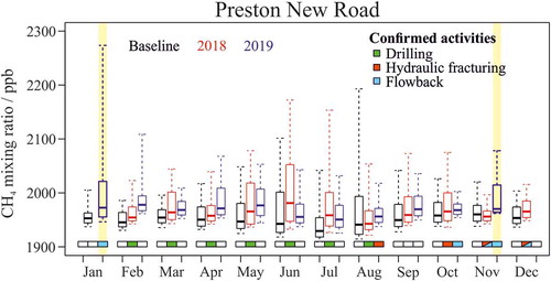
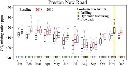
The contribution of the nitrogen gas lift in January 2019 is clearly visible, primarily in the large range in CH₄ mixing ratios up to the 90th percentile, and, to a smaller extent, up to the 75^th percentile. However, it should be noted that the median CH₄ mixing ratio was consistent with the monthly median mixing ratios to either side and with the year-on-year increase. Similar enhancements in CH₄ were potentially measured in November 2019, with a large deviation in the 75th and 90th percentile values relative to previous years, and to adjacent months. Site activity data for November 2019 reported that flowback was taking place, with successful flaring of natural gas emissions. This is potentially corroborated by Figure 6, in which a similar excursion in CO₂ statistics was observed in November 2019, potentially due to generation of CO₂ from burning of CH₄. Interestingly, no data was flagged by the change detection algorithm as breaking the threshold criteria in this month – this was likely due to the threshold criteria specifically relating to the detection of cold vented CH₄ and the lack of westerly wind directions (Figure S6). Other than during January and November 2019, no other months in which natural gas flow was reported showed obvious excursions in CH₄, or CO₂, statistics. However, enhanced monthly statistics in both CH₄ and CO₂ were potentially measured in February 2019 although no flowback operations were reported to have taken place. As for November 2019, no data from February 2019 broke the threshold criteria outlined in Shaw et al. (2019) for the detection of CH₄ excursions.

Figure 6. Boxplots for monthly CO₂ mixing ratios under westerly wind (270° ± 45°). Black boxplots show baseline period date, red boxplots show operational data measured in 2018 and blue boxplots show operational data recorded in 2019. The thick line represents the monthly median CO₂ mixing ratio, the outer edges of the boxplot shows the interquartile range, and the whiskers extend to the 10th and 90th percentile values. The rectangles toward the lower portion of the plot provides an indication of reported activities taking place at the shale gas facility during that month. Months which are highlighted showed enhancements in monthly CO₂ statistics relative to previous years and to adjacent months, potentially as a result of flowback operations. These enhancements are particularly clear in the upper extent of the whiskers (90th percentile values)

Conclusion

Enhancements in CH₄ mixing ratios were measured in January 2019 at a fixed-site monitoring station after artificial nitrogen lifting of a well (following partial hydraulic fracturing) at an onshore shale gas extraction facility in the UK. The enhancements were identified using statistically evidenced threshold criteria to detect elevations in CH₄ mixing ratios over a previously derived baseline climatology, based on both seasonality and wind direction.

Three independent methods were used to estimate CH₄ fluxes associated with the nitrogen lift emission event. Peak CH₄ fluxes were estimated to be approximately 70 g s⁻¹. However, a highly variable source strength meant that mean CH₄ fluxes were likely to be much lower, at approximately 16 g s⁻¹. The central estimate of total CH₄ mass emitted during the period was 4.2 (±1.4) tonnes CH₄, with a larger range estimated by other independent flux estimation methods (from 2.9 to 7.1 tonnes CH₄). However, these estimates do not account for potential sampling dead-time in which emissions may have been missed due to unfavorable wind directions. We note that there may be some misunderstanding in the way CH₄ emissions and CO₂-equivalent mass emission are being publicly reported. To avoid such misunderstanding in future, we recommend that the same GWP time horizon is used to convert between CH₄ mass and CO₂-equivalent, and that a singular consistent CH₄ emission value (and GWP time horizon) is publicly reported to avoid unnecessary confusion and the possibility of future greenhouse gas accounting error. Continuous monitoring and independent assessment should be sustained to ensure good practice. This study provides guidance for flux quantification from fixed-site monitoring of CH₄ sources, with implications for emissions inventory validation and public interest.

Estimates of CH₄ emissions in the exploratory phases of hydraulic fracturing, and especially during nitrogen lift operations, have not previously been made available for incorporation into environmental assessment research such as life cycle assessment (Stamford and Azapagic 2014). Based on existing LCA literature, the total CH₄ mass estimated here, for a one-week period, would be expected to result from the extraction of 1.9 Mm³ of natural gas and has an associated carbon footprint of 143 tonnes CO₂-equivalent over a 100-year time horizon (Myhre et al. 2013). It is clear from this study, and others, that emission rates associated with well development, well-unloading, and well-stimulation activities are under-represented, and may constitute a large fraction of a shale well’s lifecycle emissions. With this in mind, the UK Government should consider using Reduced Emission Completion procedures to capture flowback emissions from well-unloading and flowback operations, should onshore shale gas extraction via hydraulic fracturing continue in the future.

Acknowledgment

The information reported here has been collected as part of two complementary projects both led by the British Geological Survey (BGS): an environmental monitoring project (www.bgs.ac.uk/lancashire) jointly funded by the BGS National Capability Programme and a grant awarded by the Department for Business, Energy and Industrial Strategy (BEIS; Grant code: GA/18F/017/NEE6617R), and the Equipt4Risk project (NE/R01809X/1) which is part of the NERC/ESRC Unconventional Hydrocarbon Research Programme (www.ukuh.org). BGS authors publish with the permission of the Executive Director, BGS UKRI-UKRI.

Data availability

Calibrated data from the Environmental Baseline Project can be found on the CEDA Archive (http://www.ceda.ac.uk/) at http://catalogue.ceda.ac.uk/uuid/17381cd841ba46aca622307cdcf95da7 (Purvis, 2016).

Disclosure statement

The authors declare that they have no conflict of interest.

Supplemental material

Supplemental data for this article can be accessed on the publisher’s website.

Additional information

Funding

This work was supported by the Department for Business, Energy and Industrial Strategy [GA/18F/017/NEE6617R]; Natural Environment Research Council [NE/R01809X/1].

Notes on contributors

Jacob T. Shaw

Jacob T. Shaw is a post-doctoral research assistant at The University of Manchester working on quantifying greenhouse gas emissions from anthropogenic and natural sources.

Grant Allen

Grant Allen is a professor of atmospheric physics at The University of Manchester specialising in measurement and quantification of greenhouse gases and air quality. He can be contacted at http://[email protected].

Joseph Pitt

Joseph Pitt is a post-doctoral research associate at Stony Brook University, with a focus on quantifying greenhouse gas emissions. He was previously employed at The University of Manchester.

Adil Shah

Adil Shah was a Ph.D. student at The University of Manchester, supervised by Grant Allen, developing UAV-based methane measurement approaches and flux methods.

Shona Wilde

Shona Wilde is a Ph.D. research student at the University of York interested in the impact of emissions from the oil and gas industry on air quality.

Laurence Stamford

Laurence Stamford is a senior lecturer in sustainable chemical engineering at The University of Manchester, focusing on the sustainability assessment of energy systems and the production of foods, chemicals and materials.

Zhaoyang Fan

Zhaoyang Fan was a third year BSc Environmental Sciences student at The University of Manchester engaged in a project to study and analyse methane emissions from UK hydraulic fracturing.

Hugo Ricketts

Hugo Ricketts is a National Centre for Atmospheric Science instrument scientist at The University of Manchester with research interests including air pollution monitoring, atmospheric LIDAR and UAVs.

Paul I. Williams

Paul I. Williams is a National Centre for Atmospheric Science research scientist at The University of Manchester, who assisted with UAV-based field campaigns in this work.

Prudence Bateson

Prudence Bateson was a Ph.D. student at the Centre for Atmospheric Science at The University of Manchester researching greenhouse gas emissions from the UK offshore oil and gas industry.

Patrick Barker

Patrick Barker is a Ph.D. student at The University of Manchester, supervised by Grant Allen, researching global greenhouse gas emissions.

Ruth Purvis

Ruth Purvis is a research fellow for the National Centre for Atmospheric Science working in air quality and oil and gas emissions.

David Lowry

David Lowry is a reader in stable isotopes and greenhouse gases at Royal Holloway University London.

Rebecca Fisher

Rebecca Fisher is a lecturer in stable isotopes and greenhouse gases at Royal Holloway University London.

James France

James France is a greenhouse gas research scientist at Royal Holloway University of London and the British Antarctic Survey.

Max Coleman

Max Coleman was an MSc student in Earth Sciences at Royal Holloway, University of London. He is now pursuing a PhD in meteorology at the University of Reading.

Alastair C. Lewis

Alastair C. Lewis is professor of atmospheric chemistry at the University of York and a science director of the National Centre for Atmospheric Science. He can be contacted at http://[email protected].

David A. Risk

Dave A. Risk is a professor at St. Francis Xavier University specialising in the development and application of greenhouse gas measurement technologies for detecting and mapping fugitive emissions in Canada and the US.

Robert S. Ward

Rob S. Ward is Director of Science and Policy at the British Geological Survey. He directs the integrated programme of environmental monitoring and research that this paper is part of.

References

- Allen, D. T., D. W. Sullivan, D. Zavala-Araiza, A. P. Pacsi, M. Harrison, K. Keen, M. P. Fraser, A. D. Hill, B. K. Lamb, R. F. Sawyer, et al. 2015. Methane emissions from process equipment at natural gas production sites in the United States: Liquid unloadings. Environ. Sci. Technol. 49:641–48. doi:10.1021/es504016r.
- Allen, D. T., V. M. Torres, J. Thomas, D. W. Sullivan, M. Harrison, A. Hendler, S. C. Herndon, C. E. Kolb, M. P. Fraser, A. D. Hill, et al. 2013. Measurements of methane emissions at natural gas production sites in the United States. Proc. Natl. Acad. Sci. 110:17768–73. doi:10.1073/pnas.1304880110.
- Atherton, E., D. Risk, C. Fougère, M. Lavoie, A. Marshall, J. Werring, J. P. Williams, and C. Minions. 2017. Mobile measurement of methane emissions from natural gas developments in north-eastern British Columbia, Canada. Atmos. Chem. Phys. 17:12405–20. doi:10.10.5194/acp-17-12405-2017.
- BEIS. 2019. Greenhouse gas reporting: Conversion factors. London, UK: Department for Business, Energy & Industrial Strategy. Accessed August, 2019. https://www.gov.uk/government/publications/greenhouse-gas-reporting-conversion-factors–2019.
- Brantley, H. L., E. D. Thoma, W. C. Squier, B. B. Guven, and D. Lyon. 2014. Assessment of methane emissions from oil and gas production pads using mobile measurements. Environ. Sci. Technol. 48:14508–15. doi:10.1021/es503070q.
- Cathles, L. M., III, L. Brown, M. Taam, and A. Hunter. 2012. A commentary on “The greenhouse-gas footprint of natural gas in shale formations”; by R. W. Howarth, R. Santoro, and A. Ingraffea. Clim. Change 113 (2):525–35. doi:http://dx.doi.10.1007/s10584-011-0333-0.
- Clancy, S. A., F. Worrall, R. J. Davies, and J. G. Gluyas. 2018. An assessment of the footprint and carrying capacity of oil and gas well sites: The implications for limiting hydrocarbon reserves. Sci. Tot. Env. 618:586–94. doi:10.1016/j.scitotenv.2017.02.160.
- Connolly, P. 2019. A simple Gaussian plume model for investigating air quality. Accessed February 7, 2019. https://github.com/maul1609/gaussian-plume-model-practical.
- Cooper, J., L. Stamford, and A. Azapagic. 2014. Environmental impacts of shale gas in the UK: Current situation and future scenarios. Energy Technol. 2 (12):1012–26. doi:10.1002/ente.201402097.
- Cuadrilla Resources Ltd. 2019. Accessed June 24, 2019. https://cuadrillaresources.com/media-resources/press-releases/cuadrilla-shale-gas-initial-flow-test-results/.
- Cuadrilla Resources Ltd. 2020. Community liaison group meeting minutes. Accessed January 21, 2020. https://cuadrillaresources.uk/our-sites/preston-new-road/preston-new-road-documents/.
- Dlugokency, E. 2020. NOAA/ESRL. Accessed 29, 2020. https://esrl.noaa.gov/gmd/ccgg/trends_ch4/.
- Ecoinvent. 2018. Ecoinvent database v3.5. Zurich, Switzerland: The Ecoinvent Centre.
- Element Energy, 2019. Assessment of options to reduce emissions from fossil fuel production and fugitive emissions. Final Report for The Committee on Climate Change. Cambridge, UK. Accessed Augest 30, 2020. https://www.theccc.org.uk/publication/assessment-of-options-to-reduce-emissions-from-fossil-fuel-production-and-fugitive-emissions/.
- Environment Agency. 2019a. Environment agency: EPR compliance assessment report for preston new road exploration site EPR/AB3101MW. Report ID: UP3431VF/0328941. issued March 28, 2019. Accessed Augest 30, 2020. https://consult.environment-agency.gov.uk/onshore-oil-and-gas/information-on-cuadrillas-preston-new-road-site/supporting_documents/Preston%20New%20Road%20Compliance%20with%20Permit%20Assessment%20Report%2027.02.2019%20_%20Flare%20Operations.pdf
- Environment Agency. 2019b. personal communication. 15 August and 26 September.
- EPA. 2014. Oil and natural gas sector liquids unloading processes. U.S. EPA Office of Air Quality Planning and Standards. Accessed Augest 30, 2020. https://www.ourenergypolicy.org/wp-content/uploads/2014/04/epa-liquids-unloading.pdf
- Flesch, T. K., J. D. Wilson, and E. Yee. 1995. Backward-time Lagrangian stochastic dispersion models, and their application to estimate gaseous emissions. J. Appl. Meteorol. 34:1320–32. doi:10.1175/1520-0450(1995)034<320:btlsdm>2.0.CO;2.
- Flesch, T. K., L. A. Harper, J. M. Powell, and J. D. Wilson. 2009. Inverse dispersion calculation of ammonia emissions from Wisconsin dairy farms. Trans. ASABE 52:253–65. doi:10.13031/2013.25946.
- Foster-Wittig, T. A., E. D. Thoma, and J. D. Albertson. 2015. Estimation of point source fugitive emission rates from a single sensor time series: A conditionally-sampled Gaussian plume reconstruction. Atmos. Environ. 115:101–09. doi:10.1016/j.atmosenv.2015.05.042.
- Gu, H. 1995. Transient aspects of unloading oil and gas wells with coiled tubing. Soc. Petrol. Eng. J. SPE-29541-MS. doi:10.2118/29541-MS.
- Hausmann, P., R. Sussmann, and D. Smale. 2016. Contribution of oil and natural gas production to renewed increase in atmospheric methane (2007–2014): Top-down estimate from ethane and methane column observations. Atmos. Chem. Phys. 16:3227–44. doi:10.5194/acp-16-3227-2016.
- Howarth, R. W. 2019. Ideas and perspectives: Is shale gas a major driver of recent increase in global atmospheric methane? Biogeosciences 16:3033–46. doi:10.5194/bg-16-3033-2019.
- Hultman, N., D. Rebois, M. Scholten and C. Ramig. 2011. The greenhouse impact of unconventional gas for electricity generation. Environ. Res. Lett. 6:049504. doi:10.1088/1748-9326/4/049504.
- Jiang, M., W. M. Griffin, C. Hendrickson, P. Jaramillo, J. Van Briesen, and A. Venkatesh. 2011. Life cycle greenhouse gas emissions of Marcellus shale gas. Env. Res. Lett. 6 (3). doi: 10.1088/1748-9326/6/3/034014.
- Lowry, D., R. E. Fisher, J. L. France, M. Coleman, M. Lanoisellé, G. Zazzer, E. Nisbet, J. T. Shaw, G. Allen, J. Pitt, et al. 2020. Environmental baseline monitoring for shale gas development: Identification and geochemical characterisation of local source emissions of methane to atmosphere. Sci. Tot. Env. 708:134600. doi:10.1016/j.scitotenv.2019.134600.
- MacKay, D. J. C., and T. J. Stone. 2013. Potential greenhouse gas emissions associated with shale gas extraction and use. London: Department of Energy & Climate Change.
- Milkov, A. V., S. Schwietzke, G. Allen, O. A. Sherwood, and G. Etiope. 2020. Using global isoptic data to constrain the role of shale gas production in recent increases in atmospheric methane. Sci. Rep. 10:4199. doi:10.1038/s41598-020-61035-w.
- Myhre, G., D. Shindell, F.-M. Bréon, W. Collins, J. Fuglestvedt, J. Huang, D. Koch, J.-F. Lamarque, D. Lee, B. Mendoza, et al. 2013. Anthropogenic and natural radiative forcing. In Climate change 2013: The physical science basis. contribution of working group I to the fifth assessment report of the intergovernmental panel on climate change, ed. T. F. Stocker, D. Qin, G.-K. Plattner, M. Tignor, S. K. Allen, J. Boschung, A. Nauels, Y. Xia, V. Bex, and P. M. Midgley, 710–720. Cambridge, UK and New York, NY: Cambridge University Press.
- Nisbet, E. G., E. J. Dlugokencky, M. R. Manning, D. Lowry, R. E. Fisher, J. L. France, S. E. Michel, J. B. Miller, J. W. C. White, B. Vaughn, et al. 2016. Rising atmospheric methane: 2007–2014 growth and isotopic shift. Global Biogeochem. Cy. 30:1356–70. doi:10.1002/2016GB005406.
- O’Shea, S. J., S. J.-B. Bauguitte, M. W. Gallagher, D. Lowry, and C. J. Percival. 2013. Development of a cavity-enhanced absorption spectrometer for airborne measurements of CH4 and CO2. Atmos. Meas. Tech. 6:1095–109. doi:10.5194/amt-6-1095-2013.
- Ofgem. 2019. Typical domestic consumption values. London, UK: Office of Gas and Electricity Markets. Accessed August 14, 2019. https://www.ofgem.gov.uk/gas/retail-market/monitoring-data-and-statistics/typical-domestic-consumption-values.
- Pasquill, F. 1961. The estimation of the dispersion of wind-borne material. Meteorol. Mag. 90 (1063):33–49.
- Prinn, R. G., R. F. Weiss, J. Arduini, T. Arnold, P. J. Fraser, A. L. Ganesan, J. Gasore, C. M. Harth, O. Hermansen, J. Kim, et al. 2020. The ALE/GAGE/AGAGE data base. http://agage.mit.edu/data. or The ALE/GAGE/AGAGE Network (DB 1001), http://cdiac.ess-dive.lbl.gov/ndps/alegage.html (10.3334/CDIAC/atg.db1001).
- Purvis, R. M. 2016. Environmental baseline project: Air quality, greenhouse gas, volatile organic compounds (VOCs) and surface meteorological measurements from Kirby Misperton and Little Plumpton. Centre for Environmental Data Analysis. Accessed August, 2019. http://catalogue.ceda.ac.uk/uuid/17381cd841ba46aca622307cdcf95da7.
- Purvis, R. M., A. C. Lewis, J. R. Hopkins, S. E. Wilde, R. E. Dunmore, G. Allen, J. Pitt, and R. S. Ward. 2019. Effects of ‘pre-fracking’ operations on ambient air quality at a shale gas exploration site in rural North Yorkshire, England. Sci. Tot. Env. 673:445–54. doi:10.1016/j.scitotenv.2019.04.077.
- Rich, A., J. P. Grover, and M. L. Sattler. 2014. An exploratory study of air emissions associated with shale gas development and production in the Barnett Shale. J. Air Waste Manag. Assoc. 64:61–72. doi:10.1080/10962247.2013.832713.
- Riddick, S. N., S. Connors, A. D. Robinson, A. J. Manning, P. S. D. Jones, D. Lowry, E. Nisbet, R. L. Skelton, G. Allen, J. Pitt, et al. 2017. Estimating the size of a methane emission point source at different scales: From local to landscape. Atmos. Chem. Phys. 17:7839–51. doi:10.5194/acp-17-7839-2017.
- Rigby, M., S. A. Montzka, R. G. Prinn, J. W. C. White, D. Young, S. O’Doherty, M. F. Lunt, A. L. Ganesan, A. J. Manning, P. G. Simmonds, et al. 2017. Role of atmospheric oxidation in recent methane growth. P. Natl. Acad. Sci. USA 114:5373–77. doi:10.1073/pnas.1616426114.
- Robertson, A. M., R. Edie, D. Snare, J. Soltis, R. A. Field, M. D. Burkhart, C. S. Bell, D. Zimmerle, and S. M. Murphy. 2017. Variation in methane emission rates from well pads in four oil and gas basins with contrasting production volumes and compositions. Environ. Sci. Technol. 51:8832–40. doi:10.1021/acs.est.7b00571.
- Robinson, C., K. Driver, M. D’Antoni, R. Liu, B. Barlow, W. Funk, and A. Ravikumar. 2019. Cap-op energy British Columbia oil and gas methane emissions field study. Prepared for the British Columbia Government and Environment and Climate Change Canada. Accessed August 24, 2019. https://www2.gov.bc.ca%2Fassets%2Fgov%2Fenvironment%2Fclimate-change%2Find%2Freporting-emissions%2F2019%2Fbritish_columbia_oil_and_gas_methane_emissions_field_study.pdf&usg=AOvVaw2H9mgOGPo4_3rsAUCtTPaY.
- Saide, P. E., D. F. Steinhoff, B. Kosovic, J. Weil, N. Downey, D. Blewitt, S. R. Hanna, and L. D. Monache. 2018. Evaluating methods to measure methane emissions from oil and gas production facilities using LES simulations. Environ. Sci. Technol. 52:11206–14. doi:10.1021/acs.est.8b01767.
- Schaefer, H., S. E. Mikaloff-Fletcher, C. Veidt, K. R. Lassey, G. W. Brailsford, T. M. Bromley, E. J. Dlugokencky, S. E. Michel, J. B. Miller, I. Levin, et al. 2016. A 21st century shift from fossil-fuel to biogenic methane emissions indicated by 13CH4. Science 352:80–84. doi:10.1126/science.aad2705.
- Schwietzke, S., O. A. Sherwood, L. M. P. Bruhwiler, J. B. Miller, G. Etiiope, E. J. Dlugokencky, S. E. Michel, V. A. Arling, B. H. Vaughn, J. W. C. White, et al. 2016. Upward revision of global fossil fuel methane emissions based on isotope database. Nature 538:88–91. doi:10.1038/nature19797.
- Shah, A., H. Ricketts, J. Pitt, J. Shaw, K. Kabbabe, B. Leen, and G. Allen. 2020a. Unmanned aerial vehicle observations of cold venting from exploratory hydraulic fracturing in the United Kingdom. Env. Res. Lett. 2:021003. doi:10.1088/2515-7620/ab716d.
- Shah, A., J. R. Pitt, H. Ricketts, J. B. Leen, P. I. Williams, K. Kabbabe, M. W. Gallagher, and G. Allen. 2020b. Testing the near-field Gaussian plume inversion flux quantification technique using unmanned aerial vehicle sampling. Atmos. Meas. Tech. 13:1467–84. doi:10.5194/amt-13-1467-2020.
- Shaw, J. T., G. Allen, J. Pitt, M. I. Mead, R. M. Purvis, R. Dunmore, S. Wilde, P. Barker, P. Bateman, C. Percival, et al. 2019. A baseline of atmospheric greenhouse gases around prospective UK shale gas sites. Sci. Tot. Env. 684:1–13. doi:10.1016/j.scitotenv.2019.05.266.
- Skone, T. J. 2011. Life cycle greenhouse gas inventory of natural gas extraction, delivery and electricity production. DOE/NETL-2011/1522. National Energy Technology Laboratory. Accessed Augest 30, 2020. https://fossil.energy.gov/ng_regulation/sites/default/files/programs/gasregulation/authorizations/2012/applications/sierra_exhibits_12_100_LNG/Ex._89_-_Skone_Life_Cycle_GHG_Inventory_.pdf
- Stamford, L., and A. Azapagic. 2012. Life cycle sustainability assessment of electricity options for the UK. Int. J. Energy Res. 36:14. doi:10.1002/er.2962.
- Stamford, L., and A. Azapagic. 2014. Life cycle environmental impacts of UK shale gas. Appl. Energy 134:506–18. doi:10.1016/j.apenergy.2014.08.063.
- Turner, A. J., C. Frankenberg, P. O. Wennberg, and D. J. Jacob. 2017. Ambiguity in the causes for decadal trends in atmospheric methane and hydroxyl. P. Natl. Acad. Sci. USA 114:5367–72. doi:10.1073/pnas.1616020114.
- Turner, D. B. 1970. Workbook of atmospheric dispersion estimates, PHS publication No. 999-AP-26. US Department of Health, Education and Welfare, National Air Pollution Control Administration, Cincinnati, OH.
- United Kingdom Onshore Oil and Gas, UKOOG. 2019. Updated shale gas production scenarios. London, UK. Accessed Augest 30, 2020. https://www.ukoog.org.uk/images/ukoog/pdfs/Updated%20shale%20gas%20scenarios%20March%202019%20website.pdf.
- US EPA. 2014. Draft “Other Test Method” OTM 33 Geospatial Measurement of Air Pollution, Remote Emissions Quantifications (GMAP-REQ). Accessed June 24, 2019. https://www.epa.gov/emc.
- Vaughn, T. L., C. S. Bell, C. K. Pickering, S. Schwietzke, G. A. Heath, G. Pétron, D. J. Zimmerle, R. C. Schnell, and D. Nummedal. 2018. Temporal variability largely explains top-down/bottom-up difference in methane emission estimates from a natural gas production region. Proc. Natl. Acad. Sci. 115:11712–17. doi:10.1073/pnas.1805687115.
- Ward, R. S., P. L. Smedley, G. Allen, B. J. Baptie, M. R. Cave, Z. Daraktchieva, R. Fisher, D. Hawthorn, D. G. Jones, A. Lewis, et al. 2018. Environmental baseline monitoring project: Phase III final report. OR/18/026. British Geological Survey, Nottingham, UK. (Unpublished).
- Ward, R. S., P. L. Smedley, G. Allen, B. J. Baptie, Z. Daraktchieva, A. Horleston, D. G. Jones, C. J. Jordan, A. Lewis, D. Lowry, et al. 2017. Environmental baseline monitoring project: Phase II final report. OR/17/049. British Geological Survey, Nottingham, UK. (Unpublished).
- Weber, C. L., and C. Clavin. 2012. Life cycle carbon footprint of shale gas: Review of evidence and implications. Environ. Sci. Technol. 46 (11):5688–95. doi:10.1021/es300375n.
- Williams, P. J., M. Reeder, N. J. Pekney, D. Risk, J. Osborne, and M. McCawley. 2018. Atmospheric impacts of a natural gas development within the urban context of Morgantown, West Virginia. Sci. Tot. Env. 639:404–16. doi:10.1016/j.scitotenv.2018.04.422.
- Worden, J. R., A. A. Bloom, S. Pandey, Z. Jiang, H. M. Worden, T. W. Walter, S. Houweling, and T. Röckmann. 2017. Reduced biomass burning emissions reconcile conflicting estimates of the post-2006 atmospheric methane budget. Nat. Commun. 8:2227. doi:10.1038/s41467-017-02246-0.