Contribution of mobile sources to secondary formation of carbonyl compounds

ABSTRACT

In the 2014 National Air Toxics Assessment (NATA), the carbonyl compounds formaldehyde and acetaldehyde were identified as key cancer risk drivers and acrolein was identified as one of the three air toxics that drive most of the noncancer risk. In this assessment, averaged across the Continental United States, about 75% of ambient formaldehyde and acetaldehyde, and about 18% of acrolein, is formed secondarily. This study was conducted to estimate the potential contribution to these secondarily formed carbonyl compounds from mobile sources. To develop such estimates, we conducted several CMAQ runs, where emissions are set to zero for different mobile source sectors, to determine their potential contribution. Although zeroing out emissions from an individual sector can offer only a rough approximation of how the sector might contribute to overall secondary concentrations, our results suggest that across the U. S., mobile sources contribute about 6–18% to secondary formaldehyde, 0–10% to secondary acetaldehyde, and 0–70% to secondary acrolein, depending on location.

Implications: Photochemical modeling of carbonyl compounds was conducted with emissions set to zero for various mobile source sectors to determine their contribution to secondary concentrations. Results indicated mobile sources contributed to total and secondary concentrations of formaldehyde, acetaldehyde, and acrolein in many locations across the U.S. with acrolein the dominant contributor in some locations. However, biogenic sources dominated secondary formaldehyde and acetaldehyde, and fires dominated secondary acrolein.

Introduction

The United States Environmental Protection Agency periodically conducts National Air Toxics Assessments (NATAs). These assessments are screening analyses designed to help identify which air toxics, emission sources, and locations warrant further study. The most recent NATA was conducted for calendar year 2014 (EPA 2018a). In this assessment, the carbonyl compounds formaldehyde and acetaldehyde were identified as key cancer risk drivers (EPA 2018b). In addition, acrolein was identified as one of the three air toxics the drive most of the noncancer risk.

Previous research suggests that photochemical production accounts for most of ambient concentrations of carbonyl compounds such as formaldehyde and acetaldehyde, and a significant portion of ambient acrolein (Friedfeld et al. 2002; Liu, Jeffries, and Sexton 1999, Luecken et al., 2011). The 2014 National Air Toxics Assessment (NATA) estimated that, nationwide, about 75% of ambient formaldehyde and acetaldehyde, and about 18% of acrolein, is formed secondarily.

Methane is a dominant source of formaldehyde in some countries, and in remote locations. However, in much of the U.S., biogenic volatile organic compounds (VOCs) typically play a larger role, particularly in the Southeast (Jones et al. 2009; Luecken et al. 2012, 2018; Zhang et al. 2013). Moreover, while the global formaldehyde background is largely due to methane oxidation, emissions of other VOCs from biogenic, biomass burning and anthropogenic continental sources result in important and localized production (DeSmedt et al., 2015). In addition to methane, precursor compounds which form formaldehyde include alkenes, through reaction with ozone, methyl radicals through decomposition, alkoxy radicals through reaction with oxygen or decomposition, and methylperoxy radicals through reactions with hydroperoxy radicals and self-cross reactions (Luecken et al. 2018). Research on the global atmospheric budget for acetaldehyde suggests alkanes, alkenes, and ethanol are the main precursors to secondary acetaldehyde formation, with a minor contribution from isoprene (Millet et al. 2010). Acrolein forms secondarily by photooxidation of 1,3-butadiene and other hydrocarbons (Tuazon et al. 1999). Mobile sources contribute to secondary formation of all three of these compounds. They are key sources of alkene and alkane emissions, which react to form formaldehyde and acetaldehyde, and 1,3-butadiene, which reacts to form acrolein.

Despite the ubiquitous presence of mobile source direct emissions of these compounds, research to determine the mobile source contribution to secondary and overall concentrations of carbonyls is very limited. Recently, Luecken et al. (2018) used direct decoupled method (DDM) in the Community Multiscale Air Quality (CMAQ) model to quantify the relative role of emission sectors and individual classes of VOCs on ambient formaldehyde in the U.S. DDM calculates sensitivity coefficients which are used to predict concentrations as a result of model perturbations (Napelenok et al., 2008). The Luecken study found that in summer, biogenic sources contribute the most to hydrocarbon sensitivity across the U. S. (over 90%), whereas anthropogenic sources (primarily mobile sources and residential wood combustion) contribute more in winter (about 36% of hydrocarbon sensitivity). The study concluded that ethanol is also a minor contributor to acetaldehyde formation, despite its widespread use in the U.S. (Luecken et al. 2012). Another U. S. study (Dunker, Koo, and Yarwood 2015) used a source-apportionment method called the Path-Integral Method (PIM), which can allocate to sources the difference in concentrations between two simulations. This method was used in conjunction with the Comprehensive Air Quality Model with Extensions (CAMx), and modeling was done for a July day in 2030, with projected inventories. The study found that anthropogenic sources accounted for about 25% of total ambient formaldehyde in urban areas and 40% in rural areas. About 40% of total anthropogenic formaldehyde in the ambient air was from mobile sources. Results in both these studies may be impacted by uncertainties associated with mechanism condensation.

The purpose of this study was to estimate the potential annual average contribution of different mobile source sectors to the secondarily formed component of ambient formaldehyde, acetaldehyde, and acrolein across the United States, and to put those contributions into perspective along with contributions from biogenic sources and fires. A recent study did this type of analysis for criteria pollutants (Zawacki et al. 2018), using reactive tracers and the CAMx model, for calendar year 2025. Unfortunately, the capability to conduct source apportionment using a reactive tracer approach does not yet exist for air toxics. Instead, this study relied on a “zero out” (also often called “brute force”) approach, where emissions for individual sectors are zeroed out to evaluate their potential impact on air quality. The limitation of such an approach is that it does not account for nonlinear chemistry and because reducing a large source changes the chemical environment. Thus, actual impacts may be significantly underestimated or overestimated. At smaller emissions perturbations, the “zero out” approach can be prone to numerical noise, leading to nonphysical results. In this study, the following sectors were zeroed out in the 2014 inventory used for the National Air Toxics Assessment: (1) highway vehicles, (2) commercial marine vessels, (3) aircraft and locomotives, (4) other nonroad equipment, (5) biogenic sources, and (6) fires.

Methods

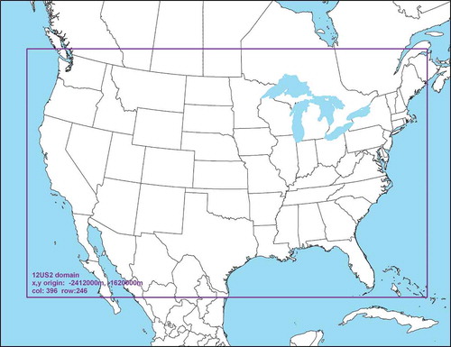
This baseline for this study was the photochemical modeling done for the 2014 NATA. This modeling used the Community Multiscale Model for Air Quality (CMAQ) version 5.2 (Appel et al. 2018), with the Carbon-Bond 6 chemical mechanism (CB06-CMAQ; Yarwood et al. 2010a, 2010b). CMAQ is a comprehensive, three-dimensional grid-based Eulerian air quality model. Meteorology inputs are based on the Weather Research Forecasting (WRF) model, version 3.8 (Skamarock et al. 2008), and processed using the Meteorology-Chemistry Interface Processor (MCIP) package, version 4.2.5 (Otte and Pliem 2010). The 2014 calendar year runs were done for the entire contiguous United States and parts of Canada and Mexico (Figure 1), using 12-km by 12-km horizontal grid spacing. Lateral boundary and initial species concentrations were provided by a three-dimensional global atmospheric chemistry model, the GEOS-Chem (Bey et al. 2001) model version 11–01.

Figure 1. Map of the CMAQ modeling domain

CB06, the current version of the carbon bond mechanism used in this assessment, is a highly condensed chemical mechanism for use in atmospheric models like CMAQ (Yarwood et al. 2010a, 2010b). CB06 models some chemical species explicitly, whereas others are broken into constituent chemical groups which have similar reactivities. Still, there are many reactions represented in CB06 leading to formation of aldehydes, and parent VOCs forming these compounds vary spatially and temporally, although alkenes in particular play a large role (Luecken et al. 2012). Yarwood et al. (2010b) found good mechanism performance for formaldehyde and acetaldehyde in chamber experiments. Nonetheless, Luecken et al. have found formaldehyde and acetaldehyde are typically underestimated in CMAQ simulations. Also, different techniques for condensing mechanisms can significantly impact formaldehyde results (Knote et al. 2015).

The main source of inventories used in 2014 NATA was the 2014 National Emissions Inventory (NEI), version 2 (EPA 2018c), which estimates emissions at the county level for U.S. states, as well as the U. S. Virgin Islands and Puerto Rico. Only inventory data for the contiguous United States were used in this study since that was the domain for photochemical modeling in 2014 NATA. Mobile source emissions for 2014, except for commercial marine vessels, locomotives and aircraft, were generated either using the MOtor Vehicle Emission Simulator, MOVES2014a (EPA 2015), or in the case of California, the EMFAC model (California Air Resources Board 2015) for highway sources and the OFFROAD model for nonroad sources. Details on methods used to develop commercial marine, locomotive, and aircraft emissions, as well as emissions from all other sources can be found in NEI documentation. Inventories were spatially allocated to grid cells and temporally allocated using the Sparse Matrix Operator Kernel Emissions (SMOKE) modeling system (Institute for the Environment – UNC Chapel Hill 2015).

A model performance evaluation was done using monitor data from the Air Toxics Archive Phase12 for the year 2014 (https://www3.epa.gov/ttnamti1/toxdat.html#data). The Atmospheric Model Evaluation Tool (AMET) was used to conduct the evaluation (Appel et al. 2011). The principal evaluation statistics used to evaluate performance in this analysis were mean bias (MB), mean error (ME), normalized mean bias (NMB), and normalized mean error (NME). Thirty monitor sites were available for acrolein and 111 sites for formaldehyde and acetaldehyde. Acrolein was ultimately excluded in the model evaluation given data uncertainty and limited sampling. Acrolein is extremely difficult to measure accurately due to post-collection reactions inside canisters (EPA 2010) . This adds additional uncertainty to interpretation of results for this pollutant. Table 1 presents annual air toxics performance statistics for formaldehyde and acetaldehyde. While modeled estimates tend to underestimate monitor values, mean bias and error were relatively moderate when compared to observations.

Table 1. CMAQ performance statistics for 2014 NATA

Pollutant	Mean Bias (MB; µg/m^3)	Mean Error (ME; µg/m^3)	Normalized Mean Bias (NMB; %)	Normalized Mean Error (NME; %)
Formaldehyde	−0.9	1.0	−41.5	45.2
Acetaldehyde	−0.3	0.5	−21.8	35.5

The following sectors were excluded in “zero out” CMAQ runs: onroad (highway vehicles), nonroad equipment (not including aircraft, rail, or commercial marine vessels), aircraft and rail, commercial marine vessels (CMVs), biogenic sources, and fires. Nonroad equipment includes lawn and garden equipment, recreational vehicles, construction equipment, agricultural and logging equipment and recreational marine vessels. The term “rail” is used to refer to locomotive emissions.

Annual average absolute concentration differences were calculated (2014 NATA CMAQ concentration minus “zero out”; eq 1)(1) $\left(2014\mathrm{N}\mathrm{A}\mathrm{T}\mathrm{A}-\mathrm{Z}\mathrm{e}\mathrm{r}\mathrm{o}\mathrm{O}\mathrm{u}\mathrm{t}\left(\mathrm{S}\mathrm{e}\mathrm{c}\mathrm{t}\mathrm{o}\mathrm{r}\mathrm{X}\right)\right)/2014\mathrm{N}\mathrm{A}\mathrm{T}\mathrm{A}$(1) as well as percent contribution for each pollutant for each grid cell:

(1) $\left(2014\mathrm{N}\mathrm{A}\mathrm{T}\mathrm{A}-\mathrm{Z}\mathrm{e}\mathrm{r}\mathrm{o}\mathrm{O}\mathrm{u}\mathrm{t}\left(\mathrm{S}\mathrm{e}\mathrm{c}\mathrm{t}\mathrm{o}\mathrm{r}\mathrm{X}\right)\right)/2014\mathrm{N}\mathrm{A}\mathrm{T}\mathrm{A}$(1)

These metrics were calculated for total concentration of the carbonyls as well as the secondary contribution only. In addition, we calculated the fractional contribution to average nationwide secondary carbonyl concentrations for mobile source sectors across grid cells, at the 5th, 25th, 50th, 75th, and 95th percentiles.

Results and discussion

Inventory contributions

Table 2 presents the contributions of mobile source sectors, as well as biogenic, fire, and stationary source emissions, to the total primary emissions of the three carbonyls for the 2014 NATA. Mobile source contributions for formaldehyde, acetaldehyde and acrolein are 6%, 5% and 12%, respectively. Stationary sources also contribute, with 4%, 3% and 10%. Direct emissions are dominated by biogenic sources and fires (agricultural field burning, prescribed fires and wildfires collectively) for formaldehyde and acetaldehyde, and by fires for acrolein. There are no biogenic direct emissions of acrolein.

Table 2. Short tons of emissions from mobile source, biogenic source, and stationary source sectors in 2014 NATA

Sector	Formaldehyde (% Total)	Acetaldehyde (% Total)	Acrolein (% Total)
Onroad	35,327 (2.89)	25,832 (3.19)	2,323 (4.54)
Commercial Marine Vessels	1,064 (0.08)	515 (0.06)	21 (0.04)
Aircraft	4,830 (0.39)	1662 (0.21)	945 (1.85)
Rail	1,112 (0.09)	483 (0.06)	80 (0.16)
Other Nonroad	35,756 (2.92)	14,147 (1.75)	2,542 (4.97)
Total Mobile	78,089 (6.38)	42,639 (5.27)	5,911 (11.55)
Biogenic	855,346 (69.90)	627,243 (77.50)	0
Fires	237,163 (19.38)	117,704 (14.54)	40,317 (78.81)
Stationary	52,997 (4.33)	21,811 (2.70)	4,930 (9.64)
All Sources	1,223,595	809,397	51,158

Contributions to total ambient concentrations

Table 3 provides the fractional contribution of mobile source, biogenic, and fire emissions to grid cell ambient concentration at various percentiles. Stationary sources can be assumed to account for the remainder of ambient concentrations. Biogenic sources make the largest contribution among sectors for formaldehyde and acetaldehyde (52 and 80%, respectively, at the 50th percentile), while fires make the largest contribution for acrolein (54% at the 50th percentile). At the 50^th percentile, a little less than 10% of ambient formaldehyde is from mobile sources, increasing to over 17% at the 95th percentile. For commercial marine vessels, while the sector contributes only a little over 3% at the 50th percentile, it contributes almost 18% at the 95th percentile, reflecting the large impact of major ports. Mobile sources are smaller contributors to ambient levels of acetaldehyde, although they account for about 10% at the 95th percentile. Negative values at lower percentiles could indicate that emissions from that sector are destroying carbonyls or alternatively, can be attributed to nonlinearity of chemical reactions. As discussed above, at smaller emissions perturbations, the “zero out” approach can be prone to numerical noise, leading to nonphysical results. Although emissions of ethanol, a precursor of acetaldehyde, have increased significantly in recent years with the use of 10% ethanol gasoline, air quality modeling results do not suggest much impact on ambient acetaldehyde on regional scales (Cook et al. 2011; Luecken et al. 2012). However, localized impacts may be larger where the contribution of direct emissions play a greater role. In contrast to formaldehyde and acetaldehyde, mobile sources are much larger contributors to ambient levels of acrolein, accounting for over 17% at the 50th percentile and almost 60% at the 95th percentile. This is because mobile sources account for a large portion of 1,3-butadiene emissions across the United States, approximately 36% (EPA 2018c), and these emissions form acrolein secondarily.

Table 3. Contribution of mobile source sectors to total ambient concentrations of carbonyls

Percentile	5%	25%	50%	75%	95%
Formaldehyde
Air/Rail	0.002	0.005	0.007	0.0100	0.018
CMV	0	0.0005	0.003	0.051	0.180
Onroad	0.022	0.041	0.057	0.077	0.111
Nonroad	0.007	0.014	0.020	0.032	0.055
Total Mobile	0.044	0.072	0.095	0.123	0.174
Biogenic	0.362	0.459	0.518	0.584	0.668
Fires	0.004	0.012	0.025	0.047	0.121
Acetaldehyde
Percentile
Air/Rail	−0.010	−0.007	−0.004	−0.002	0.000
CMV	−0.052	−0.014	−0.002	−0.001	0.000
Onroad	−0.031	−0.012	−0.001	0.015	0.057
Nonroad	−0.001	0.001	0.008	0.020	0.058
Total Mobile	−0.041	−0.017	0.000	0.028	0.105
Biogenic	0.575	0.712	0.802	0.855	0.918
Fires	0.009	0.020	0.040	0.064	0.139
Acrolein
Percentile
Air/Rail	−0.007	0.005	0.018	0.033	0.084
CMV	−0.343	−0.018	−0.003	−0.001	0.000
Onroad	−0.029	0.026	0.081	0.164	0.296
Nonroad	0.005	0.030	0.066	0.119	0.259
Total Mobile	−0.026	0.064	0.172	0.330	0.582
Biogenic	0.007	0.025	0.047	0.079	0.155
Fires	0.103	0.280	0.536	0.774	0.946

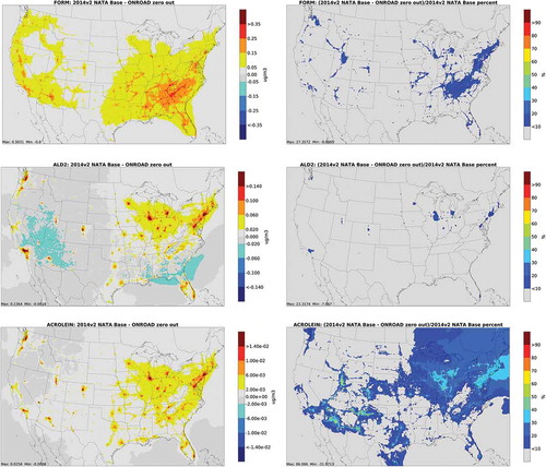
Figure 2 depicts annual average absolute concentration differences and percent differences from onroad zero out runs for carbonyls. Base case total and secondary concentrations are depicted in Figures S1 and S2 of the supplemental information. For formaldehyde, impacts are greatest in the Southeast and major metropolitan areas. These impacts are consistent with formaldehyde column measurements which show the highest isoprene concentrations in the Southeastern U. S. (Millet et al. 2009), and the hypothesis that there is interaction between mobile source precursors and biogenic pollutants such as isoprene. For acetaldehyde, impacts are greatest in large urban areas and along major transportation corridors. A similar (Figures S3 through 25) pattern is seen for acrolein.

Figure 2. Absolute total concentration differences (column 1) and percent differences (column 2) from onroad zero out runs for carbonyls (FORM = formaldehyde; ALD2 = acetaldehyde)

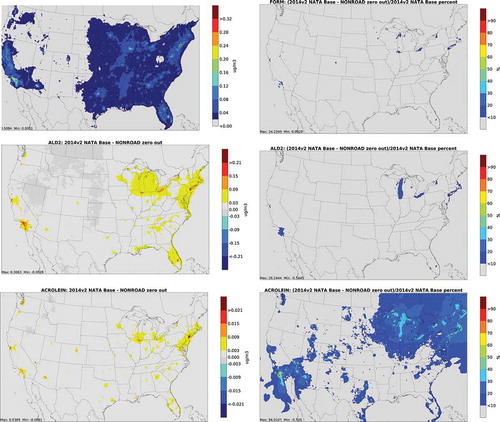
Figure 3 depicts annual average absolute concentration differences and percent differences from nonroad zero out runs for carbonyls. The largest impacts for carbonyls occur near population centers, particularly in urban areas with significant recreational marine activity. In addition, nonroad has a larger contribution to percent differences for acrolein in Northern Michigan, Wisconsin and Minnesota. This may be due to activity from recreational marine equipment in summer. Snowmobile activity is also substantial in this region during winter but less likely to make a major contribution due to lower photooxidation.

Figure 3. Absolute total concentration differences (column 1) and percent differences (column 2) from nonroad zero out runs for carbonyls (FORM = formaldehyde; ALD2 = acetaldehyde)

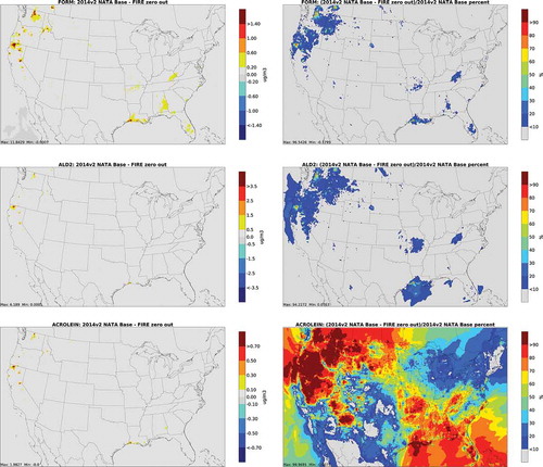
Figures 4 and Figures 5 depict annual average absolute concentration differences and percent differences from biogenic and fire zero out runs for carbonyls. For biogenic sources, the largest impacts for formaldehyde and acetaldehyde are in the montane forests of the Southwest and in the Deep South. The largest concentration differences for acrolein are in the Northwest and Deep South, although the largest percent differences are offshore. In 2014, the largest impact of fires on carbonyl emissions was in the Pacific Northwest.

Figure 4. Absolute total concentration differences (column 1) and percent differences (column 2) from biogenic zero out runs for carbonyls (FORM = formaldehyde; ALD2 = acetaldehyde)

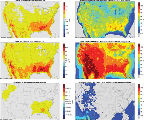
Figure 5. Absolute total concentration differences (column 1) and percent differences (column 2) from fire zero out runs for carbonyls (FORM = formaldehyde; ALD2 = acetaldehyde)

Figures for the CMV and rail/aircraft zero out runs are included in the Supplemental Material. For CMV, impacts on carbonyl concentrations are largest along the West Coast, Gulf Coast, and South Atlantic Coast, where most marine ports are located. For acrolein from air and rail, impacts are greatest in large urban areas, and along certain heavily trafficked rail lines. There is very little impact from this sector on formaldehyde and acetaldehyde concentrations.

Contributions to secondary ambient concentrations

Table 4 provides the fractional contribution to grid cell secondary concentrations at various percentiles. As with total concentrations, biogenic sources make the largest contribution among sectors for secondary formaldehyde and acetaldehyde (41% and 78%, respectively, at the 50th percentile), while fires make the largest contribution for acrolein (41% at the 50th percentile). While there are no direct biogenic emissions of acrolein, biogenic sources account for almost 15% of secondarily formed acrolein. At the 50th percentile, about 12% of ambient formaldehyde is from mobile sources, increasing to over 18% at the 95th percentile. As with total ambient acetaldehyde, mobile sources are smaller contributors than formaldehyde to secondary levels. Because of atmospheric transformation of 1,3-butadiene to acrolein, mobile sources account for over 35% of acrolein at the 50th percentile and over 70% at the 95th percentile.

Table 4. Contribution of mobile source sectors to secondary concentrations of carbonyls

Percentile	5%	25%	50%	75%	95%
Formaldehyde
Air/Rail	0.002	0.005	0.009	0.013	0.022
CMV	0	0.001	0.004	0.057	0.187
Onroad	0.028	0.050	0.072	0.094	0.126
Nonroad	0.009	0.018	0.023	0.033	0.051
Total Mobile	0.058	0.0907	0.118	0.147	0.182
Biogenic	0.299	0.364	0.410	0.483	0.598
Fires	0.004	0.010	0.018	0.028	0.072
Acetaldehyde
Percentile
Air/Rail	−0.012	0.008	−0.005	0.003	−0.001
CMV	−0.051	−0.014	−0.003	−0.001	0.000
Onroad	−0.033	−0.013	−0.002	0.013	0.044
Nonroad	−0.001	0.002	0.009	0.022	0.062
Total Mobile	−0.043	−0.019	0.000	0.027	0.095
Biogenic	0.563	0.689	0.783	0.836	0.900
Fires	0.009	0.023	0.037	0.056	0.118
Acrolein
Percentile
Air/Rail	−0.014	0.002	0.013	0.020	0.041
CMV	−0.307	−0.023	−0.005	−0.002	0.000
Onroad	−0.010	0.109	0.217	0.307	0.419
Nonroad	0.026	0.076	0.112	0.180	0.345
Total Mobile	0.010	0.201	0.355	0.508	0.718
Biogenic	0.051	0.087	0.147	0.206	0.270
Fires	0.087	0.235	0.410	0.636	0.861

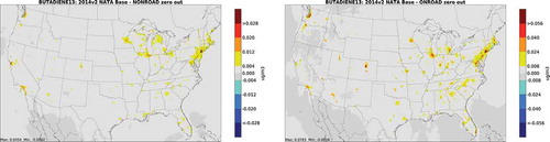
Figure 6 depicts annual average absolute secondary concentration differences and percent differences from onroad zero out runs for carbonyls, and Figure 7 depicts differences from nonroad zero out runs. Not surprisingly, geographic patterns are similar  to total concentration differences, given the dominance of secondary carbonyls over primary. Even for secondary concentrations, concentrations are greater in urban centers and along transportation corridors. This is not unexpected, given emissions of alkene and 1,3-butadiene precursor emissions associated with onroad and nonroad sources. The distribution of differences for secondary acrolein is very similar to 1,3-butadiene, its primary precursor compound (Figure 8). Figures for the biogenic, fire, CMV and rail/aircraft zero out runs are included in the Supplemental Material (Figures S6 through S8). For CMV, impacts on carbonyl concentrations are largest along the West Coast, Gulf Coast, and South Atlantic Coast. For acrolein and acetaldehyde from aircraft and rail, impacts are greatest in large urban areas, and along certain heavily trafficked rail lines. For biogenic and fire sources, spatial distribution of secondary concentrations is similar to that of total emissions.

Figure 6. Absolute secondary concentration differences (column 1) and percent differences (column 2) from onroad zero out runs for carbonyls (FORM = formaldehyde; ALD2 = acetaldehyde)

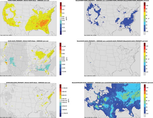
Figure 7. Absolute secondary concentration differences (column 1) and percent differences (column 2) from nonroad zero out runs for carbonyls (FORM = formaldehyde; ALD2 = acetaldehyde)

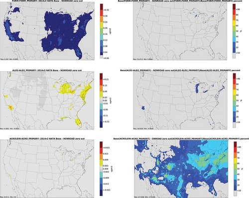
Figure 8. Absolute concentration differences from onroad and nonroad zero out runs for 1,3-butadiene, acrolein precursor

It should be noted that there are many sources of uncertainty in the inventory and air quality modeling done for the NATA assessment on which this analysis is based. Sources of uncertainty include magnitude and location of emissions from various sources, chemical speciation of compounds of interest, meteorological characterization, and treatment of chemistry and transport. These sources of uncertainty should be considered when interpreting results. They are discussed in detail in the technical support document for 2014 NATA (EPA 2018b). In addition, as discussed previously, there are significant limitations in the “zero out” approach used in this study. Examining linearity of results by modeling different levels of reductions for mobile source sectors could inform this issue. Moreover, because most of the U. S. population is concentrated in a small fraction of the grid cells modeled, these ambient concentration results do not reflect which source sectors are contributing most to secondary exposures. Also, fire emissions vary substantially from year to year; thus, results could be significantly different in another year, although fire emissions were not atypical in 2014 (Urbanski et al. 2018). Finally, this analysis does not account for seasonal differences, which are substantial due to photooxidation.

Summary

Mobile sources contribute to total and secondary concentrations of formaldehyde, acetaldehyde, and acrolein in many locations across the U.S. with acrolein the dominant contributor in some locations. However, biogenic sources dominate secondary formaldehyde and acetaldehyde, and fires dominated secondary acrolein. In some locations, however, mobile sources contribute substantially to secondary acrolein concentrations due to atmospheric transformation of 1,3-butadiene. It should be noted that this modeling only captures average concentrations in 12 square kilometer grid cells. Primary carbonyl emissions may be substantial contributors to ambient concentrations in close proximity to large sources of mobile source emissions, such as major roads, ports, and freight terminals (Clements, et al. 2009; Health Effects Institute 2010). Because of limitations with the “zero out” approach, a reactive tracer approach should be developed for carbonyls compounds to better understand contributions of mobile sources, stationary sources and biogenic sources to secondary concentrations.

Disclaimer

The views expressed in this article are those of the authors and do not necessarily represent the views or policies of the U.S. Environmental Protection Agency.

Disclosure statement

No potential conflict of interest was reported by the authors.

Supplementary material

Supplemental data for this article can be accessed on the publisher’s website.

Additional information

Notes on contributors

Rich Cook

Rich Cook is a physical scientist in the Assessment and Standards Division of the Office of Transportation and Air Quality, Office of Air and Radiation, U. S. Environmental Protection Agency.

Sharon Phillips

Sharon Phillips is a physical scientist in the Air Quality Assessment Division of the Office of Air Quality Planning and Standards, Office of Air and Radiation, U. S. Environmental Protection Agency.

Madeleine Strum

Madeleine Strum is an environmental engineer in the Air Quality Assessment Division of the Office of Air Quality Planning and Standards, Office of Air and Radiation, U. S. Environmental Protection Agency.

Alison Eyth

Alison Eyth is an environmental engineer in the Air Quality Assessment Division of the Office of Air Quality Planning and Standards, Office of Air and Radiation, U. S. Environmental Protection Agency.

James Thurman

James Thurman is a physical scientist in the Air Quality Assessment Division of the Office of Air Quality Planning and Standards, Office of Air and Radiation, U. S. Environmental Protection Agency.

References

- Appel, K. W., S. Napelenok, C. Hogrefe, G. Pouliot, K. M. Foley, S. J. Roselle, J. E. Pleim, J. Bash, H. O. T. Pye, N. Heath, et al. 2018. Overview and evaluation of the community multiscale air quality model (CMAQ) modeling system version 5.2. In Air Pollution Modeling and its Application XXV. ITM 2016. Springer Proceedings in Complexity, eds. C. Mensink and G. Kallos, Cham, Switzerland: Springer. Accessed May 23, 2019. doi:10.1007/978-3-319-57645-9_11.
- Appel, K. W., R. C. Gilliam, N. Davis, A. Zubrow, and S. C. Howard. 2011. Overview of the atmospheric model evaluation tool (AMET) v1.1 for evaluating meteorological and air quality models. Environ. Model. Software 26 (4):434–43. doi:10.1016/j.envsoft.2010.09.007.
- Bey, I., D. J. Jacob, R. M. Yantosca, J. A. Logan, B. D. Field, A. M. Fiore, Q. Li, H. Y. Liu, L. J. Mickley, and M. G. Schultz. 2001. Global modeling of tropospheric chemistry with assimilated meteorology: Model description and evaluation. J. Geophys. Res. 106:23073. doi:10.1029/2001JD000807.
- California Air Resources Board. 2014. EMFAC2014. Accessed May 23, 2019. https://ww3.arb.ca.gov/msei/categories.htm.
- Clements, A. L., Y. Jia, A. Denbleyker, E. McDonald-Buller, M. P. Fraser, D. T. Allen, D. R. Collins, E. Michel, J. Pudota, D. Sullivan, et al. 2009. Air pollutant concentrations near three Texas roadways, part II: Chemical characterization and transformation of pollutants. Atmos. Environ. 43:4523–34. doi:10.1016/j.atmosenv.2009.06.044.
- Cook, R., S. Phillips, M. Houyoux, P. Dolwick, R. Mason, C. Yanca, M. Zawacki, K. Davidson, H. Michaels, C. Harvey, et al. 2011. Air quality impacts of increased use of ethanol under the United States’ energy independence and security act. Atmos. Environ. 45:7714–24. doi:10.1016/j.atmosenv.2010.08.043.
- De Smedt, I., T. Stavrakou, F. Hendrick, T. Danckaert, T. Vlemmix, G. Pinardi, N. Theys, C. Lerot, C. Gielen, C. Vigouroux, et al. 2015. Diurnal, seasonal and long-term variations of global formaldehyde columns inferred from combined OMI and GOME-2 observations. Atmos. Chem. Phys. Discuss. 15:12241–300. doi:10.5194/acpd-15-12241-2015.
- Dunker, A. M., B. Koo, and G. Yarwood. 2015. Source apportionment of the anthropogenic increment to ozone, formaldehyde, and nitrogen dioxide by the path-integral method in a 3D model. Environ. Sci. Technol. 49:6751–59. doi:10.1021/acs.est.5b00467.
- Friedfeld, S., M. Fraser, K. Ensor, S. Tribble, D. Rehle, D. Leleux., and F. Tittel. 2002. Statistical analysis of primary and secondary atmospheric formaldehyde. Atmos. Environ 36 (30):4767–75. doi:10.1016/S1352-2310(02)00558-7.
- Health Effects Institute. 2010. Special report 17: Traffic-related air pollution: a critical review of the literature on emissions, exposure, and health effects. January. Accessed July 11, 2019. https://www.healtheffects.org/system/files/SR17Traffic%20Review.pdf.
- Institute for the Environment - UNC Chapel Hill. 2015. SMOKE v3.6.5 user’s manual. Accessed May 23, 2019. https://www.cmascenter.org/smoke/documentation/3.6.5/html/
- Jones, N. B., K. Riedel, W. Allan, S. Wood, P. I. Palmer, K. Chance, and J. Notholt. 2009. Long-term tropospheric formaldehyde concentrations deduced from ground-based fourier transform solar infrared measurements. Atmos. Chem. Phys. 9:7131–42. doi:10.5194/acp-9-7131-2009.
- Knote, C., P. Tuccella, G. Curci, L. Emmons, J. Orlando, S. Madronich, R. Baro, P. Jimeenez-Guerrero, D. Luecken, C. Hogrefe, et al. 2015. Influence of the choice of gas-phase mechanism on predictions of key gaseous pollutants during AQMEII phase-2 intercomparison. Atmos. Environ. 115:553–68. doi:10.1016/j.atmosenv.2014.11.066.
- Liu, X., H. E. Jeffries, and K. G. Sexton. 1999. Hydroxyl radical and ozone initiated photochemical reactions of 1,3-butadiene. Atmos. Environ. 33 (18):3005–22. doi:10.1016/S1352-2310(99)00078-3.
- Luecken, D. J., S. L. Napelenok, M. Strum, R. Scheffe, and S. Phillips. 2018. Sensitivity of ambient atmospheric formaldehyde and ozone to precursor species and source types across the United States. Environ. Sci. Technol. 52:4668–75. doi:10.1021/acs.est.7b05509.
- Luecken, D. J., W. T. Hutzell, M. L. Strum, and D. J. Pouliot. 2012. Regional sources of atmospheric formaldehyde and acetaldehyde, and implications for atmospheric modeling. Atmos. Environ. 47 (2012):477–90. doi:10.1016/j.atmosenv.2011.10.005.
- Millet, D. B., A. Guenther, D. Siegel, N. Nelson, H. Singh, J. De Gouw, C. Warneke, J. Williams, G. Eerdekens, V. Sinha, et al. 2010. Global atmospheric budget of acetaldehyde: 3-D model analysis and constraints from in-situ and satellite observations. Atmos. Chem. Phys. 10:3405–25. doi:10.5194/acp-10-3405-2010.
- Millet, D. B., D. J. Jacob, K. F. Boersma, T. Fu, T. P. Kurosu, K. Chance, and C. L. H. A. Guenther. 2009. Spatial distribution of isoprene emissions from North America derived from formaldehyde column measurements by the OMI satellite sensor. J. Geophys. Res. 113:D02307. doi:10.1029/2007JD008950.
- Napelenok, S. L., D. S. Cohan, M. T. Odman, and S. Tonse. 2008. Extension and evaluation of sensitivity analysis capabilities in a photochemical model. Environ. Mod. Software 23:994–99. doi:10.1016/j.envsoft.2007.11.004.
- Otte, T. L., and J. E. Pleim. 2010. The Meteorology-Chemistry Interface Processor (MCIP) for the CMAQ modeling system: updates through MCIPv3.4.1. Geosci. Model Dev. 3:243–256. doi:10.1.1.617.7579.
- Skamarock, W. C., J. B. Klemp, J. Dudhia, D. O. Gill, D. M. Barker, M. G. Duda, X. Huang, W. Wang, and J. G. Powers. 2008. A Description of the Advanced Research WRF Version 3. NCAR Tech. Note NCAR/TN-475+STR.
- Tuazon, E. C., A. Alvarado, S. M. Aschmann, R. Atkinson, and J. Arey. 1999. Products of the gas-phase reactions of 1,3-butadiene with OH and NO3 radicals. Environ. Sci. Technol. 33 ((20)):3586–95. doi:10.1021/es990193u.
- U.S. Environmental Protection Agency (EPA). 2010. Data quality evaluation guidelines for ambient air acrolein measurements. Accessed May 14, 2020. http://www.epa.gov/ttnamti1/files/ambient/airtox/20101217acroleindataqualityeval.pdf.
- U.S. Environmental Protection Agency (EPA). 2015. https://www.epa.gov/moves/previous-moves-versions-and-documentation.
- U.S. Environmental Protection Agency (EPA). 2018a. 2014 National air toxics assessment. Accessed May 21, 2019. https://www.epa.gov/national-air-toxics-assessment.
- U.S. Environmental Protection Agency (EPA). 2018b. Technical support document: EPA’s 2014 national air toxics assessment. Office of air quality planning and standards, Research Triangle Park, NC, August. Accessed May 21, 2019. https://www.epa.gov/sites/production/files/2018-09/documents/2014_nata_technical_support_document.pdf.
- U.S. Environmental Protection Agency (EPA). 2018c. 2014 National emissions inventory, version 2: Technical support document. Accessed May 23, 2019. https://www.epa.gov/sites/production/files/2018-07/documents/nei2014v2_tsd_05jul2018.pdf.
- Urbanski, S. P., M. C. Reeves, R. E. Corley, R. P. Silverstein, and W. M. Hao. 2018. Contiguous United States wildland fire emission estimates during 2003–2015. Earth Syst. Sci. Data 10 (4):2241–74. doi:10.5194/essd-10-2241-2018.
- Yarwood, G., J. Jung, G. Z. Whitten, G. Heo, J. Mellberg, and M. Estes. 2010a. Updates to the carbon bond mechanism for version 6 (CB6). Presented at 9th Annual CMAS Conference, Chapel Hill, NC, October 11-13. Accessed May 23, 2019. https://www.cmascenter.org/conference/2010/abstracts/emery_updates_carbon_2010.pdf.
- Yarwood, G., G. Z. Whitten, J. Jung, G. Heo, and D. T. Allen. 2010b. Development, evaluation and testing of version 6 of the carbon bond chemical mechanism (CB6). Prepared by Environ Corp. for the Texas Commission on Environmental Quality. Accessed May 13, 2019. https://www.tceq.texas.gov/assets/public/implementation/air/am/contracts/reports/pm/5820784005FY1026-20100922-environ-cb6.pdf
- Zawacki, M., K. Baker, S. Phillips, K. Davidson, and P. Wolfe. 2018. Mobile source contributions to ambient ozone and particulate matter in 2025. Atmos. Environ. 188:129–41. doi:10.1016/j.atmosenv.2018.04.057.
- Zhang, H., J. Li, Q. Ying, B. B. Guven, and E. P. Olaguer. 2013. Source apportionment of formaldehyde during TexAQS 2006 using a source-oriented chemical transport model. J. Geophys. Res.: Atmos. 118:1525–35. doi:10.1002/jgrd.50197.