Plume analysis from field evaluations of a portable air quality monitoring system

ABSTRACT

Near-road measurements in Rochester, NY with a Portable Air Quality Monitoring System indicate a significant plume control of PM_2.5 black carbon (BC) concentrations. This study evaluates the performance of two portable air quality enclosures deployed at collocated research sites to determine their accuracy and usefulness in field deployments, and specifically in pollution plume analysis. One system deployed collocated sensors for measurement of particulate matter mass concentration (Thermo pDR 1500 against Tapered Element Oscillating Microbalance (TEOM) measurement) and the second system deployed sensors for measurement of black carbon (Magee AE33 aethalometer and Brechtel Tricolor Absorption Photometer) in ambient and near-road locations in Rochester, New York, respectively. While the optical PM_2.5 sensors tended to be biased in their determination of concentration by ~15%, they followed changes and trends in concentration very well. The black carbon sensors in the portable systems agreed very well with each other and with the collocated sensor. As a case study to determine the contribution from statistically significant short-lived excursions of pollutant concentration, Morlet wavelet analysis was performed on data from the portable system sensors. Black carbon was found to be strongly influenced by plume behavior with significant plume excursions representing just over 12% of all data points and contributing on average 1 µg/m³ of black carbon above ambient concentrations.

Implications: This paper first evaluates two air pollutant monitoring enclosures with wide applicability including near-road detection of pollutants. Then, we present a novel method to designate isolate statistically significant excursions in air pollution concentration which can be used to determine the impact of pollutant plumes as observed in PM and black carbon behavior near road.

Introduction

Exposure to ambient air pollution is known to be hazardous to human health, with outdoor air pollution causing an estimated 3.9 million premature deaths worldwide annually (Lelieveld et al. 2015). This risk is mainly attributed to fine particulate matter (PM) with a diameter of 2.5 µm or smaller (PM_2.5) and is typically measured by PM_2.5 mass which is an EPA criterion pollutant with a primary annual standard of 12 µg/m³ and a primary daily standard of 35 µg/m³ which is considered adequate as maximum concentrations for general public health concerns. Specifically, black carbon (BC) as a component of PM_2.5 has been highlighted as a possible source for PM toxicity upon inhalation, with increases in black carbon per unit mass being demonstrably hazardous for human health and distinct from total PM_2.5 mass (Atkinson et al. 2015; Janssen et al. 2012). While PM and black carbon concentrations are known to fluctuate rapidly with movement of particle-laden plumes, most health and exposure studies rely on 24 h (or longer) averaged exposure times, possibly misrepresenting exposure in environments such as near road where individual sources can generate rapid fluctuations in pollutant concentration (e.g. Atkinson et al. 2015; Hamra et al. 2014; Shah et al. 2015). In this study, pollutant plumes are specifically defined as a significant sustained excursion above random variability in pollutant concentration.

With advancing technology, there has been a proliferation of optical sensors for measurement of air pollutants. These sensors are often small, portable, lower in cost than alternative systems, and highly responsive to rapid changes in pollutant concentration. Availability of these sensors has allowed for new styles of scientific inquiry to flourish in the field of air quality with an emphasis on highlighting their applicability while acknowledging their shortcomings (Collier-Oxandale et al. 2020; Feenstra et al. 2019; Hagan et al. 2018; Morawska et al. 2018; Wang et al. 2015; Williams et al. 2019). Whereas many monitoring agencies have constructed permanent field measurement sites equipped with robust, stationary equipment, present infrastructure is oftentimes inadequate to quantify the high degree of spatial and temporal variability of air pollutants for rapidly changing exposure (Feinberg et al. 2019; Kumar et al. 2015; Li et al. 2019). This shortcoming becomes increasingly important when considering impacts of pollutant operating on extremely localized scales (e.g. Saha et al. 2019) or in measurement situations that are impractical for large-scale equipment, such as near-road environments or near pollutant disaster sites (e.g. Subramanian et al. 2018). Thus, optical PM sensors have been used in a variety of situations to supplement stationary measurements, including numerous studies using low-cost sensors for community-wide sensing (e.g. Bhattacharya, Sridevi, and Pitchiah 2012; North et al. 2009; Shusterman et al. 2016; White et al. 2012) and multiple traffic studies for assessing near-road exposure and risks (e.g. Askariyeh, Zietsman, and Autenrieth 2020; Canagaratna et al. 2010; Deville Cavellin et al. 2015; Padró-Martínez et al. 2012).

In response to this changing paradigm, we have built eight portable air quality monitor (PAQM) enclosures for use in highly localized air pollution scenarios. Each PAQM consists of an insulated enclosure outfitted with various optical sensors specifically for measurement of PM_2.5 and black carbon. For this study, two of the PAQMs were deployed to Rochester, New York for a field evaluation and comparison to sensors operating at established air quality monitoring sites including a near-road site. This paper serves to demonstrate the effectiveness of these optical sensors against field standards, and – as a case study to demonstrate the applicability of this data – specific time series of pollutants are analyzed with novel methods to describe distinct plume activity and characterize trends in transport and exposure to PM and BC.

Methods

For this study, two portable air quality monitors (PAQMs) were deployed to two New York State Department of Environmental Conservation (NYS DEC) field sites in Rochester, New York. The PAQM units were part of a series of eight designed for flexible, rapid deployment and ease of continuous measurement of air quality parameters. Enclosures consisted of a customized chassis by American Products (AM-462418-24RU; 1.17 m high by 0.61 m wide by 0.46 m deep) outfitted with electronics, stainless steel sample inputs, and limited capability to regulate temperature with a heater and fan, as well as a computer for on-site data collection. Each enclosure was outfitted with a LUFFT WS500-UMB Smart Weather Sensor, a Panasonic Toughbook laptop, and an Omron temperature controller for internal temperature regulation.

The PAQMs were deployed at two NYS DEC continuous measurement sites; the Rochester main site (hereafter the main site or MS in figures) which is located at 30 Yarmouth Road, Rochester, NY (43°08ʹ46.3”N, 77°32ʹ53.6”W), and the Rochester Near Road site (hereafter the near-road site or NR in figures) which is directly adjacent to interstate 490 (43°08ʹ42.0”N, 77°33ʹ27.3”W). The main site location contained flat terrain with surroundings including a three-story apartment complex, trees, and elevated railroad tracks all at least 40 m from the PAQM. The PAQM was stationed on a wooden deck at around 1 m above ground level with inlets approximately 3 m above ground level. The near-road site was at the upper edge of a parking lot with the PAQM placed on top of a monitoring shelter, elevating the inlets approximately 15 m above the highway roadway and less than 1 m horizontally to the edge of the roadway. Aerial photographs of the sites can be seen in supplemental Figure 1 and photographs of the near-road PAQM can be seen in supplemental Figure 5.

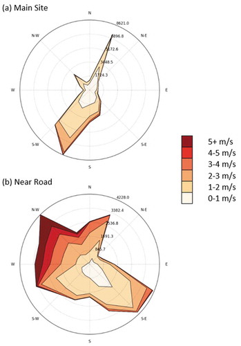
Figure 1. 5-minute wind plots for the main site(a) and near road site (b) for 16 direction bins. Color indicates the wind speed and distance from the center indicates frequency

The PAQM at the main site was equipped with two optical light-scattering instruments for particulate matter (PM) detection; a Thermo personal data RAM (pDR 1500), which is a handheld nephelometer. The pDR is a commonly used portable instrument for rapid industrial PM detection which, in this study, was equipped with a cyclone for size selection of particulate matter smaller than a 2.5-micron diameter size cut (PM_2.5). The pDR used a manufacturer recommended environmental calibration coefficient to convert an optical signal into a mass concentration which is optimized for particles of mass median aerodynamic diameter between 2 and 3 μm, with a refractive index of 1.54.

In addition to its own pDR sensor, the near-road PAQM contained two optical filter-based black carbon sensors, a Magee AE33 Aethalometer (Aeth in figures) and a Brechtel Tricolor Absorption Photometer (hereafter TAP). Each of these instruments detects black carbon by measuring the absorption of light at various wavelengths through a suspension of particles collected on a filter. By quantifying additional light absorption over time with known airflow rates, wavelength-dependent absorption coefficients, and assumed particle densities; these instruments compute a mass loading rate for particulate matter absorbing light at specific wavelengths. The aethalometer measures absorption at 7 wavelengths of light, where absorption at 880 nm is assumed to be solely due to black carbon, and the TAP measures absorption at 3 wavelengths of light where absorption also at 640 nm was assumed to be black carbon. The TAP measurement was scaled down by 15% to correct the absorption coefficient to attain agreement with the aethalometer (see Liang et al. 2019)

While not discussed here, the main site PAQM was also equipped with a TSI Environmental DustTrak DRX (DRX) for supplemental PM measurement with limited size resolution. The PAQMs were designed for flexible deployment with additional sensors available for use including AlphaSense CO and NO₂ sensors and Xontech 901 canister sampler for collection of VOCs.

Both PAQM units were deployed from March 22 until September 30, 2016. The PAQMs were continuously and independently operational 24 hours a day for the entire testing period and any missing data is instrument dependent. Typically, the PAQMs were left unattended for two-week intervals between routine maintenance and data collection and occasional tests of various instrument configurations account for most missing data. All data were collected at a 1-min sampling frequency. One-minute data were then averaged into 5-min data for construction of wind roses and 1-h data for comparison with DEC instruments which reported hourly values.

Analysis was performed in Python using built-in statistical functions. For the purposes of instrument comparison, two factor Deming regression was used to determine linearity of response across all instruments (based on theory in Saylor, Edgerton, and Hartsell 2006). Comparisons were performed between PAQM deployed instruments in addition to instruments at the collocated DEC sites. For DEC PM measurements, each site was equipped with a Tapered Element Oscillating Microbalance (TEOM), which is a gravimetric PM sensor. For DEC black carbon measurements both sites were also equipped with their own AE33 Aethalometer (labeled as DEC BC in figures).

As a case study to demonstrate the usefulness of these datasets, a novel application of wavelet analysis was then used for both pDRs and the near-road PAQM aethalometer to determine periods of significant plume activity as adapted from the methodology described in detail in Torrence and Compo (1998) by determining when pollutant concentration sustained an exceeded concentration that was significantly above variability in the concentration for a similar time scale. This case study acts to show the applicability of a single time series high time resolution data from data sources such as the PAQMs.

Wavelets are mathematical functions that have been used in various environmental applications to determine the timing and scale of aperiodic features within a time series. Test wavelets are transcribed across time series data to determine how much signal power resides at any given point in the time series. By dilating the wavelet, this method can describe how well features of various frequencies or equivalent periods are present in the data. Complex wavelets cast time series data into the complex plane, simultaneously revealing scale and frequency of features at any given time. Wavelets have previously been used for various atmospheric applications such as analysis of El Niño/South oscillations, complex oceanic wave and wind interactions, and for turbulence studies (Domingues, Mendes, and Mendes da Costa 2005; Gao and Li 1993).

As a complex wavelet, the Morlet wavelet allows for precise quantification of signal energy within a time series due to its combination of real and complex components and large amount of oscillations. The Morlet wavelet is described mathematically as a complex sinusoid fitted to a Gaussian bell curve that is normalized to the scale of the data. Oscillations within the sinusoid closely resemble a Fourier period for a windowed Fourier transform on the scale of the daughter wavelet and describe features resembling cosine waves within the equivalent period within the data. In this case, the Morlet wavelet is used to determine the signal power of pollutant concentration at any given point in time within the dataset. Since the Morlet wavelet transform determines features based on the scaling of the daughter wavelet, it performs a mathematical isolation of features within the dataset irrespective of features of different sizes. Furthermore, and important for plume analysis, this allows for determination of statistically significant activity within the dataset for various time scales determined entirely from a single time series of pollutant data.

For data segments longer than 2 weeks, minute concentration data were interrogated using Morlet wavelets with equivalent Fourier frequencies growing from 2 minutes by powers of 2 for 12–15 levels depending on the length of the data segment. Significance was determined by performing a chi-square significance test for wavelet power as compared to a white-noise background spectrum for the data (Torrence and Compo 1998). This result was used to determine periods of significant short-term plume activity, which was specifically defined as time periods containing significant wavelet power at the 95% confidence level for any wavelet periods of 60 minutes or less. When supplementing the time series of the data, this criterion allowed for quantitative designation of short-lived peaks in concentration as significantly above stochastic variations in the data. For the time series, significance was considered in two ways. Significance at longer wavelet periods were considered to be background-controlled. In terms of pollutant concentration, this can be thought of as the slow-changing trends in concentration due to variations on relevant time scales from diurnal to seasonal, attributable to changes in characteristics such as weather, wind patterns, and regional pollutant emission. Significance at shorter wavelet periods were considered plume-controlled, wherein variations on the orders of hours to minutes would be caused by sensors detecting pollutant concentration on a more localized scale, ranging from the concentration gradient within a typical Gaussian plume (representing significance on the order of hours) down to the rapid fluctuations in concentration due to a heavily emitting passing truck or other nearby source (representing significance on the order of minutes). Morlet wavelet analysis was performed on the pDR data for both sites and on the near road aethalometer data. After computation, periods of significant plume activity were then compared to the rest of the data to better describe the impact of plume behavior on pollutant concentration. Likewise, the occurrence of these events was used to describe the distribution of the relevant pollutant as plume-controlled or background-controlled.

Results

Meteorological conditions

Monitoring was continuous throughout the entire campaign between March 22 and September 30, 2016 with minimal data interruption except for sporadic maintenance of specific instruments and approximately 1 month of downtime for the main site pDR. Temperatures varied from an hourly minimum of −7.2° C on April 5 to an hourly maximum of 34.2°C on July 13, with an hourly mean temperature of 17.5°C for the sampling period following typical diurnal and seasonal trends typical for New York state. PAQM temperatures were very strongly correlated between the two sites (slope 1.01, r² = 0.99) and PAQM relative humidity showed a similar relationship (slope 0.99, r² = 0.98). 5-minute wind data indicate a stark difference between the two sites (Figure 1). The main site experienced weak winds, typically less than 3 m/s with a strong tendency to channel in either direction along an NNE/SSW trajectory. Contrastingly, the near-road site experienced a broader array of wind speeds and directions and, in general, higher wind speeds than the main site. This wind discrepancy can be explained by the differences in terrain features for the sites (supplemental Figure 1) as well as the difference in elevation of the sensor inlets above ground level and helps define the microclimate and expected air pollutant exposure for each site.

PM_2.5

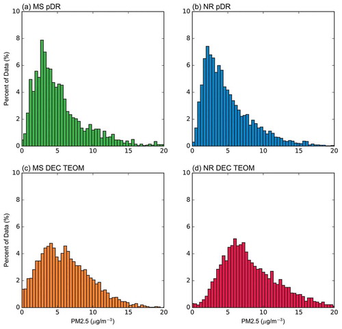
For the course of the campaign, pDR measurements were well below air quality regulation levels with an hourly averaged maximum of 19.89 µg/m³ found at the Near Road Site at 22:00 on April 17, 2016. Mean values from the optical sensors for both sites were found to be just above and below 5.1 µg/m³ with a lower median near 4.1 µg/m³ (Table 1). Correlation between the PAQM pDR and the DEC TEOM measurements at the main site (Figure 2(a)) was moderate (slope 1.15, r² = 0.65) while a very similar regression slope and a significant y-intercept for the near-road site (Figure 2(b)) indicates that the near-road TEOM had a strong tendency to report values higher than the near-road pDR (slope 1.18, r² = 0.80, intercept 2.40). PM_2.5 measurements by both pDRs were highly consistent for both sites throughout the entire study (Figure 2(c)). The strong correlation between the pDRs at the two sites (slope 1.07, r² = 0.94) indicates that optically, particle measurements were not especially different between the two sites. This relationship is also shown by the similarity between histogram of mass concentration distributions of measured PM_2.5 concentrations (Figure 3). Histograms for both the near road and main site pDRs follow a skewed distribution with a mode around 2.5 µg/m³ representing around 8% of the data whereas both TEOM instruments report broader histograms.

Table 1. Mean and median values for all the PM sensing instruments for all data points collected by the instruments and the 1623 hours when all five instruments were recording (indicated by mean* and median*) to account for any biases due to downtimes for the instruments. The main site pDR had fewer data points due to instrument malfunction and subsequent removal from the field for much of June and July. All concentrations are given in µg/m^3.

	N	Mean	Median	Mean*	Median*
MS pDR	2601	5.22	4.22	4.46	3.71
NR pDR	4286	5.01	4.07	4.21	3.58
MS DRX	3700	4.73	4.13	4.14	3.67
MS DEC TEOM	4038	6.04	5.70	5.63	5.30
NR DEC TEOM	4595	8.17	7.40	7.60	7.12

Figure 2. Deming regression correlation plots for main site PM_2.5 measurements (a), near-road PM_2.5 measurements (b), comparison between the near road and main site pDRs (c), and near-road TAP and aethalometer (d). All axes are given in μg/m³

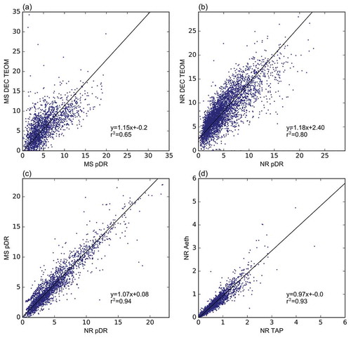
Figure 3. Histograms of the hourly average PM_2.5 concentrations for the main site pDR (a) and near-road pDR (b) as compared to the main site DEC TEOM (c) and near-road DEC TEOM (d)

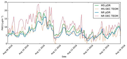
From the DEC TEOM measurements, the near-road site experienced characteristically higher PM_2.5 mass loadings while the main site measured consistently lower with an average difference of around 2 µg/m³ between the two. Data from all three optical instruments typically fell under these two DEC measurements. All three optical sensors gave time series that resembled each other and were similar to the near-road TEOM measurement, though scaled differently (Figure 4).

Figure 4. Seven-day segment of the hourly averaged PM_2.5 time series for August 9–16, 2016 as an example of trending for the main site and near-road pDRs and DEC TEOM instruments

Black carbon

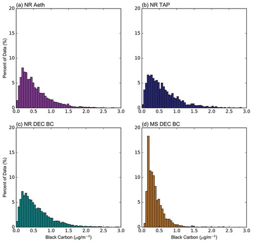
The PAQM aethalometer, TAP, and near-road DEC BC aethalometer were all in strong agreement with each other. Correlation between the TAP and the PAQM aethalometer shows very strong agreement (slope 0.97, r² = 0.93; Figure 2(d)) while the near-road DEC and the PAQM aethalometer had near identical results with less variability (slope 0.98, r² = 0.97; supplemental Figure 2). Table 2 indicates that the median hourly BC concentrations were low, typically at or below 1 µg/m³ during the field campaign. Hourly averaged black carbon concentration distributions follow a positively skewed distribution with nearly identical shape for the three near-road measurements (Figure 5(a, b, and c)) and a much thinner distribution with a smaller median concentration for the main site measurements (Figure 5(d)). While hourly values for black carbon were low, concentrations would fluctuate rapidly (on the order of minutes) from concentrations on the order of tenths of a µg/m³ to tens of µg/m³.

Table 2. Median values for each month for each black carbon instrument. All concentrations are given in µg/m^3.

	March	April	May	June	July	August	September	Overall
NR Aeth	0.380	0.306	0.462	0.423	0.530	0.496	0.524	0.451
NR TAP	0.394	0.352	0.439	0.402	0.565	0.488	0.553	0.472
NR DEC	0.407	0.319	0.466	0.424	0.556	0.512	0.520	0.467
MS DEC	0.250	0.220	0.329	0.302	0.360	0.351	0.364	0.310

Figure 5. Histograms of the hourly average black carbon concentrations for the near-road PAQM aethalometer (a), near-road PAQM TAP (b), and near-road DEC aethalometer (c) as compared by the main site DEC aethalometer (d)

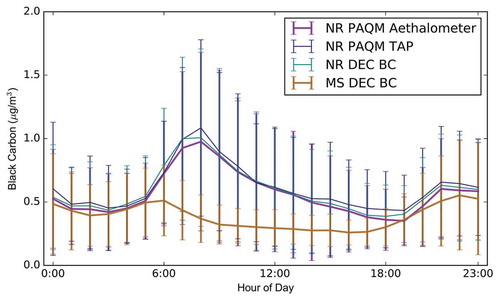
Figure 6 shows that the diurnal trend of hourly black carbon concentration displays a prominent spike around 8:00 with a large amount of variability observed in all three near-road instruments but not at the main site, suggesting a regular commuter signal. All four instruments appeared to be in reasonably good agreement with each other at night between 18:00 and 5:00 for much of the campaign, though between the hours of 6:00 and 18:00 the main site DEC black carbon measurement is characteristically lower than any of the near-road measurements.

Figure 6. Diurnal pattern of black carbon for the near-road aethalometer, near-road TAP, and the near road and main site DEC aethalometers. Bars represent one standard deviation and the line represents the mean value for each hour

Plume analysis

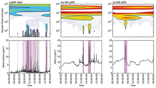
As shown by Figure 7, and more thoroughly in the supplemental Figure 3, wavelet analysis of the near-road aethalometer, near-road pDR, and main site pDR indicate that concentrations were controlled primarily by activity acting for wavelet periods on the order of one day or longer. This indicates that much of the significant variation in pollutant concentration operated at a regional or larger scale, with background sources and sinks controlling this variation. However, to differing degrees, all three instruments demonstrated significant variation in concentration on sub-hourly time periods indicative of plume behavior as previously described (Figure 7). This significant variability suggests short-term pollutant transport to the sensors either through local emissions or by rapidly changing concentration within larger plumes.

Figure 7. Segments of the wavelet scalograms (top row) with periods of significant wavelet activity at the 95% confidence interval outlined and in full opacity; and time series plots of raw minute data with times of significant plume activity highlighted with purple vertical lines (bottom row) for the near-road aethalometer (a), near-road pDR (b), and main site pDR (c) on August 19, 2016. Scalogram scale represents the base 10 log of the wavelet power where the darkest blue represents wavelet power on the scale of 10¹ and the darkest red represents power on the scale of 10⁹. In the lower plots, purple bars are constructed by selecting any minute when there is significant wavelet activity for wavelet periods of 1 hour or less

Table 3 outlines the extent to which each instrument observed plume activity. Both the main site and near-road pDR experienced a small number of significant pollutant concentration excursions, indicating that these are fringe events for PM_2.5 exposure in these microenvironments. However, periods of significant PM_2.5 activity lasted on average around 80 minutes and 120 minutes for the near road and main site, respectively, indicating continuous significant variation within these time scales. Likely, these are descriptive of variations occurring with transport within the gradient of a larger Gaussian plume across the sensors. During these plume events concentrations of PM_2.5 were approximately double the concentrations experienced for all non-plume event times, while still being well below air quality standard concentrations.

Table 3. Results indicating the percent of minute-data that is considered as significant plume data, the number, and length of continuous plume events, and the mean concentrations for both plume and non-plume times. All concentrations are given in µg/m^3.

	Percent of data as plumes (%)	Number of plume events	Average plume event length (minutes)	Mean plume concentration	Mean non-plume concentration
MS pDR	1.19	15	124.3	10.83	5.16
NR pDR	2.55	82	80.2	8.90	4.92
NR Aeth	12.25	1881	17.1	1.43	0.45

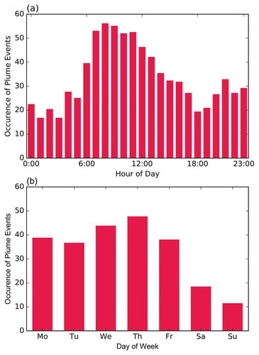
The aethalometer frequently experienced statistically significant fluctuations on short time scales, with over 12% of the data being considered as plume behavior. Aethalometer concentration excursions were shorter-lived, lasting on average just around 17 minutes. This is thought to be due to variations in black carbon emissions directly from the roadway. During periods of significant plume activity, the aethalometer observed black carbon concentrations approximately 1 µg/m³ higher than during periods without significant plume activity, on average more than tripling exposure to black carbon. Aethalometer plume behavior followed weekly and diurnal trends that were not observed as strongly with the pDR instruments (Figure 8; supplemental Figure 4). Significant plume activity was more than twice as likely to occur during weekdays than on weekends and followed a similar diurnal trend to concentrations of black carbon as observed in Figure 6.

Figure 8. Percent occurrence of diurnal (a) and day-of-week (b) occurrence of plume events for the near road for each day or hour of data measurement

Discussion

Considering that the two sites are located approximately 1 km from each other, the discrepancy between the wind data, yet consistency for other meteorological measurements, indicates a disparity between their microenvironments and suggests a difference in fresh pollutant exposure, specifically for pollutants coming from the roadway.

Measurements of PM_2.5 represent values typical for a clean nonurban environment (Seinfeld and Pandis 2006), and do not suggest that these areas of Rochester, New York are at risk for violation of state and federal regulation guidelines. While the optical instruments agreed strongly with each other, there are known shortcomings to their use for PM detection (Kulkarni and Baron 2011). The environmental scale factor for optical detection is inadequate for measurement of PM with changing composition, which is likely the case due to fluctuating black carbon concentrations from roadway sources, a PM component which the sensors cannot detect. Lab results demonstrate that these sensors will underestimate mass concentration under a high organic loading ratio and overestimate mass concentration under high inorganic ratio (Zhang, Marto, and Schwab 2018). This partially explains the tendency for the optical measurements to fall under the mass-based TEOM measurements and for the main site pDR to report higher concentrations than the near-road pDR; likely the main site PM is relatively higher in inorganic mass, with a strong contribution from black carbon felt mostly at the near-road site. Whereas the TEOM is insensitive to the effect due to changes in the scattering components between the two sites, the pDRs characteristically underestimate black carbon which is a major mass contributor at the near-road site while overestimating inorganic mass which is dominant at the main site.

As a confounding factor for the optical measurements, perhaps more important than particle composition is the size of particles being measured. Optical particle sensors are known to be highly sensitive to particle size. Optical detection efficiency operates as a function of the wavelength of the instrument’s laser compared to the size of particles throughout various scattering regimes (Wang et al. 2015). Vehicles on the roadway act as a source for fresh particle emissions which are typically high in number concentration and smaller than 100 nm in diameter (Zhang et al. 2004); sizes that are less sensitively detected by the optical instruments. Particles from vehicle exhaust are then rapidly diluted as they are transported away from the roadway leading to drastic drops in concentration within a few hundred meters of a roadway (Canagaratna et al. 2010). The combination of these two factors helps to explain discrepancies between the TEOM measurements and the pDR measurements at the two sites.

While the optical instruments are known to misestimate the PM mass, their measurements appear to be more internally stable than the TEOM measurements. Specifically, during periods of low concentration, the main site TEOM would fluctuate to physically impossible negative concentrations which were removed from analysis. This may be an artifact of TEOM measurement methods, wherein particles are heated before measurement, removing semi-volatile components of PM mass (Schwab et al. 2006). Measurements from the pDRs can also describe rapid changes in concentration on the order of minutes whereas the TEOM measurements are better suited for longer averaging periods.

The black carbon instrument results show that black carbon is a pollutant that does not demonstrate a high degree of spatial homogeneity for this scale. While both the aethalometer and the TAP adequately represent black carbon mass loadings, the TAP required filter replacements approximately once every three weeks due to filter loading. This indicates that the TAP, while a much smaller instrument, is more suited for short-term deployments, deployments in cleaner environments, or deployments with very regular maintenance.

Results from the wavelet case-study analysis indicate that short-lived spikes in pollutant concentration intermittently control exposure. For black carbon this is especially powerful, as over 12% of the time the aethalometer reported statistically significant plume concentrations of – on average – 1 µg/m³ higher than background-controlled concentrations, which has shown evidence of association with several short-term changes in health, though on a longer time scale (Janssen et al. 2012). While virtually all black carbon health studies rely on 1 h or longer exposure times, black carbon plumes are characteristically shorter than an hour in length, often lasting minutes. As health studies become attuned to shorter exposure times, the importance of rapid fluctuations in black carbon concentration will become critical in understanding exposure, such as exposure during a daily commute. Since over 12% of the data fell into the plume category, the black carbon near-road signal is considered heavily plume controlled.

It is important to note that plume activity has a high likelihood of occurring at the same times of day when the highest near-road concentrations of black carbon were measured. The difference between times with or without significant plume activity leads to the high error in the diurnal concentration of black carbon during the middle of the day. Since this behavior was not seen in the diurnal concentrations of black carbon at the main site it can be assumed that the main site black carbon concentration is not nearly as influenced by rapidly changing concentration as the near-road concentration and that the approximately 1 km between the sites is an adequate distance to remove substantial variability within the black carbon component of PM.

Neither pDR indicated regularity in plume activity to the extent of the aethalometer. This suggests that the PM_2.5 concentration at any given time is predominantly background controlled with occasional plume behavior. The average observed plume event lengths of 80 and 124 minutes for the near road and main site pDRs, respectively, also indicate that the PM plumes have independent behavior from the black carbon plumes. For the black carbon, plumes from traffic emissions could be from a handful of highly polluting vehicles and take just a few minutes to pass over the sensor, which is corroborated by the fact that much of the significant aethalometer plume activity is for wavelet behavior at periods of less than 10 minutes. For the pDRs the significant wavelet power was generally representative of plumes between 10 minutes and 1 h, indicating a slower-moving, larger air mass of elevated PM_2.5 concentration passing over the sensor.

The PAQMs displayed reasonable estimations of air pollution parameters, even when considering the shortcomings of measurements by optical PM sensors. The enclosure-based measurement system described here will allow for the identification of trends in pollutant concentration in a wide array of unique environments which were previously more difficult to assess for air quality. As a novel analysis method, wavelet analysis for determination of short-lived, yet significant, spikes in concentration proves to be useful in describing pollutant transport and for better determination of trends as well as explaining why trends exist.

Highlights

• Black carbon in a near-road environment is highly influenced by pollutant plume activity, leading to elevated concentrations for short exposure times.

• Optical PM and black carbon sensors show good agreement with established monitors.

• Statistically, significant pollutant plumes are present for ambient PM and black carbon.

Acknowledgment

The authors would like to thank Maxime Gorson, Janie Schwab, George Allen, Dirk Felton, Mike Abbot, Mike Costello, and Patricia Fritz for assistance with the design, construction, and deployment of the PAQM systems.

Disclosure statement

No potential conflict of interest was reported by the authors.

Supplementary material

Supplemental data for this article can be accessed on the publisher’s website.

Additional information

Funding

This work was funded by the New York State Energy Research and Development Authority (NYSERDA), contract number 34612A.

Notes on contributors

Joseph P. Marto

Joseph P. Marto is a Ph.D. candidate at the University at Albany in the Department of Atmospheric and Environmental Sciences in Albany, New York, USA.

Jie Zhang

Jie Zhang is a Postdoctoral Researcher at Colorado State University, Department of Atmospheric Science, Fort Collins, CO, USA.

James J. Schwab

James J. Schwab is a Research Professor and Senior Research Associate with the Atmospheric Sciences Research Center at the University at Albany. His research group studies atmospheric chemistry and air pollution, with an emphasis on policy-relevant scientific work. His research team makes continuous and ongoing measurements of air pollution at locations across New York State. His stations in the Adirondacks and Southern Tier have been continuously monitoring for thirty plus and almost twenty-five years respectively. He has also been involved in and organized field campaigns and projects to measure chemically important trace gases and aerosols, mainly across New York State.

References

- Askariyeh, M. H., J. Zietsman, and R. Autenrieth. 2020. Traffic contribution to PM2. 5 increment in the near-road environment. Atmos. Environ. 224:117113. doi:10.1016/j.atmosenv.2019.117113.
- Atkinson, R. W., A. Analitis, E. Samoli, G. W. Fuller, D. C. Green, I. S. Mudway, H. R. Anderson, and F. J. Kelly. 2015. Short-term exposure to traffic-related air pollution and daily mortality in London, UK. Nature 26:125–32. doi:10.1038/jes.2015.65.
- Bhattacharya, S., S. Sridevi, and R. Pitchiah. 2012. Indoor air quality monitoring using wireless sensor network, International Conference on Sensing Technology, IEEE. doi:10.1109/ICSensT.2012.6461713.
- Canagaratna, M. R., T. B. Onasch, E. C. Wood, S. C. Herndon, J. T. Jayne, R. C. Miake-Lye, C. E. Kolb, and D. R. Worsnop. 2010. Evolution of vehicle exhaust particles in the atmosphere. J. Air Waste Manage. Assoc. 60 (10):1192–203. doi:10.3155/1047-3289.60.10.1192.
- Collier-Oxandale, A., B. Feenstra, V. Papapostolou, H. Zhang, M. Kuang, B. Der Boghossian, and A. Polidori. 2020. Field and laboratory performance evaluations of 28 gas-phase air quality sensors by the AQ-SPEC program. Atmos. Environ. 220:117092. doi:10.1016/j.atmosenv.2019.117092.
- Deville Cavellin, L., S. Weichenthal, R. Tack, M. S. Ragettli, A. Smargiassi, and M. Hatzopoulou. 2015. Investigating the use of portable air pollution sensors to capture the spatial variability of traffic related air pollution. Environ. Sci. Technol. 50:313–20. doi:10.1021/acs.est.5b0423.
- Domingues, M. O., O. Mendes Jr, and A. Mendes da Costa. 2005. On wavelet techniques in atmospheric sciences. Adv. Space Res. 35 (5):831–42. doi:10.1016/j.asr.2005.02.097.
- Feenstra, B., V. Papapostolou, S. Hasheminassab, H. Zhang, B. Der Boghossian, D. Cocker, and A. Polidori. 2019. Performance evaluation of twelve low-cost PM2. 5 sensors at an ambient air monitoring site. Atmos. Environ. 216:116946. doi:10.1016/j.atmosenv.2019.116946.
- Feinberg, S. N., R. Williams, G. Hagler, J. Low, L. Smith, R. Brown, D. Garver, M. Davis, M. Morton, J. Schaefer, et al. 2019. Examining spatiotemporal variability of urban particulate matter and application of high-time resolution data from a network of low-cost air pollution sensors. Atmos. Environ. 213:579–84. doi:10.1016/j.atmosenv.2019.06.026.
- Gao, W., and B. L. Li. 1993. Wavelet analysis of coherent structures at the atmosphere-forest interface. J. Appl. Meteorol. 32 (11):1717–25. doi:10.1175/1520-0450(1993)032<1717:WAOCSA>2.0.CO;2.
- Hagan, D. H., G. Issacman-VanWertz, J. P. Franklin, L. M. M. Wallace, B. D. Kocar, C. L. Heald, and J. H. Kroll. 2018. Calibration and assessment of electrochemical air quality sensors by co-location with regulatory-grade instruments. Atmos. Meas. Tech. 11 (1):315–28. doi:10.5194/amt-11-315-2018.
- Hamra, G. B., N. Guha, A. Cohen, F. Laden, O. Raaschou-Nielsen, J. M. Samet, P. Vineis, F. Forastiere, P. Saldiva, T. Yorifuji, et al. 2014. Outdoor particulate matter exposure and lung cancer: A systematic review. Environ. Health Perspect. 112. doi:10.1289/ehp/1408092.
- Janssen, N. A. H., M. E. Gerlofs-Nijland, T. Lanki, R. O. Salonen, F. Cassee, G. Hoek, P. Fischer, B. Brunekreef, and M. Krzyzanowski. 2012. Health effects of black carbon. Copenhagen Ø, Denmark: World Health Organization.
- Kulkarni, P., and P. A. Baron. 2011. An approach to performing aerosol measurements, aerosol measurement: Principles, techniques, and applications. 3rd ed., 55–65. doi:10.1002/9781118001684.ch5.
- Kumar, P., L. Morawska, C. Martani, G. Biskos, M. Neophytou, S. Di Sabatino, M. Bell, L. Norford, and R. Britter. 2015. The rise of low-cost sensing for managing air pollution in cities. Environ. Int. 75:199–205. doi:10.1016/j.envint.2014.11.019.
- Laing, J. R., D. A. Jaffe, and A. J. Sedlacek. 2019. Comparison of filter-based absorption measurements of biomass burning aerosol and background aerosol at the Mt. Bachelor Observatory. Aerosol Air Qual. Res. 19 (BNL-212177-2019-JAAM). https://doi.org/10.4209/aaqr.2019.06.0298
- Lelieveld, J., J. S. Evans, M. Fnais, D. Giannadaki, and A. Pozzer. 2015. The contribution of outdoor air pollution sources to premature mortality on a global scale. Nature 525:367–74. doi:10.1038/nature15371.
- Li, H. Z., P. Gu, Q. Ye, N. Zimmerman, E. S. Robinson, R. Subramanian, J. S. Apte, A. L. Robinson, and A. A. Presto. 2019. Spatially dense air pollutant sampling: Implications of spatial variability on the representativeness of stationary air pollutant monitors. Atmos. Environ. X:2. doi:10.1016/j.aeaoa.2019.100012.
- Morawska, L., P. K. Thai, X. Liu, A. Asumadu-Sakyi, A. Bartonova, A. Bedini, F. Chai, B. Christensen, M. Dunbabin, J. Gao, et al. 2018. Applications of low-cost sensing technologies for air quality monitoring and exposure assessment: How far have they gone? Environ. Int. 116:286–99. doi:10.1016/j.envint.2018.04.018.
- North, R., J. Cohen, S. Wilkins, M. Richards, N. Hoose, J. Polak, M. Bell, P. Blythe, B. Sharif, J. Neasham, et al. 2009. Field deployments of the environmental monitoring. Traffic Eng. Control 50:484–88. http://www.scopus.com/inward/record.url?scp=73349126757&partnerID=8YFLogxK.
- Padró-Martínez, L. T., A. P. Patton, J. B. Trull, W. Zamore, D. Brugge, and J. L. Durant. 2012. Mobile monitoring of particle number concentration and other traffic-related air pollutants in a near-highway neighborhood over the course of a year. Atmos. Environ. 61:253–64. doi:10.1016/j.atmosenv.2012.06.088.
- Saha, P. K., N. Zimmerman, C. Malings, A. Hauryliuk, Z. Li, L. Snell, R. Subramanian, E. Lipsky, J. S. Apte, A. L. Robinson, et al. 2019. Quantifying high-resolution spatial variations and local source impacts of urban ultrafine particle concentrations. Sci. Total Environ. 655:473–81. doi:10.1016/j.scitotenv.2018.11.197.
- Saylor, R. D., E. S. Edgerton, and B. E. Hartsell. 2006. Linear regression techniques for use in the EC tracer method of secondary organic aerosol estimation. Atmos. Environ. 40 (39):7546–56. doi:10.1016/j.atmosenv.2006.07.018.
- Schwab, J. J., H. D. Felton, O. V. Rattigan, and K. L. Demerjian. 2006. New York state urban and rural measurements of continuous PM2. 5 mass by FDMS, TEOM, and BAM. J. Air Waste Manage. Assoc. 56 (4):372–83. doi:10.1080/10473289.2006.10464523.
- Seinfeld, J. H., and S. N. Pandis. 2006. Atmospheric chemistry and physics: From air pollution to climate change. 2nd ed. Hoboken, NJ: Wiley.
- Shah, A. S. V., K. Ken Lee, D. A. McAllister, A. Hunter, H. Nair, W. Whiteley, J. P. Langrish, D. E. Newby, and N. L. Mills. 2015. Short term exposure to air pollution and stroke: Systematic review and meta-analysis. BMJ 350. doi:10.1136/bmj.h1295.
- Shusterman, A. A., V. E. Teige, A. J. Turner, C. Newman, J. Kim, and R. C. Cohen. 2016. The BErkeley atmospheric CO2 observation network: Initial evaluation. Atmos. Chem. Phys. 16 (21):13449–63. doi:10.5194/acp-16-13449-2016.
- Subramanian, R., A. Ellis, E. Torres-Delgado, R. Tanzer, C. Malings, F. Rivera, M. Morales, D. Baumgardner, A. Prest, and O. L. Mayol-Bracero. 2018. Air quality in puerto rico in the aftermath of hurricane maria: A case study on the use of lower cost air quality monitors. ACS Earth Space Chem. 2 (11):1179–86. doi:10.1021/acsearthspacechem.8b00079.
- Torrence, C., and G. P. Compo. 1998. A practical guide to wavelet analysis. Bull. Am. Meteorol. Soc. 79:61–78. doi:10.1175/1520-0477(1998)079<0061:APGTWA>2.0.CO;2.
- Wang, Y., J. Li, H. Jing, Q. Zhang, J. Jiang, and P. Biswas. 2015. Laboratory evaluation and calibration of three low-cost particle sensors for particulate matter measurement. Aerosol. Sci. Technol. 49:1063–77. doi:10.1080/02786826.2015.1100710.
- White, R. M., I. Paprotny, F. Doering, W. E. Cascio, P. A. Solomon, and L. A. Gundel. 2012. Sensors and ‘apps’ for community-based: Atmospheric monitoring. EM Air Waste Manage. Assoc. Mag. Environ. Managers 36–40. doi:10.3390/s17112478.
- Williams, R., R. Duval, V. Kilaru, G. Hagler, L. Hassinger, K. Benedict, J. Rice, A. Kaufman, R. Judge, G. Pierce, et al. 2019. Deliberating performance targets workshop: Potential paths for emerging PM2. 5 and O3 air sensor progress. Atmos. Environ. X:2. doi:10.1016/j.aeaoa.2019.100031.
- Zhang, J., J. P. Marto, and J. J. Schwab. 2018. Exploring the applicability and limitations of selected optical scattering instruments for PM mass measurement. Atmos. Meas. Tech. 11 (5):2995. doi:10.5194/amt-11-2995-2018.
- Zhang, K. M., A. S. Wexler, Y. Fang Zhu, W. C. Hinds, and C. Sioutas. 2004. Evolution of particle number distribution near roadways. Part II: The ‘Road-to-Ambient’ process. Atmos. Environ. 38 (38):6655–65. doi:10.1016/j.atmosenv.2004.06.044.