A robust method for collecting and processing the on-road instantaneous data of fuel consumption and speed for motorcycles

ABSTRACT

Using the laboratory-based fuel consumption models for predicting real-world fuel consumption requires the measurement of data under certain conditions to obtain high accuracy of predicted result. Therefore, it is necessary to develop a logging device for measuring the real-time fuel consumption and speed of vehicle on the road. This article presents a study on developing the on-board data logging device to collect real-world data of fuel consumption and speed for motorcycles with the update rate of 1 Hz. The instantaneous speed of the motorcycle was determined based on the rotational speed of the wheel and the wheel radius. Another module was used to determine the instantaneous fuel consumption rate (FR) though measuring the duration injection pulse. The relationship between the duration injection pulse and the injected amount of fuel was established with high correlation coefficient of 0.997. In addition, a filter was designed to remove noise in the dataset collected using the data logging device. The random errors in the speed and the FR profiles were detected and replaced, the percentage of these errors is 1.8% and 2.4%, respectively. The developed method is a precise one for transient fuel consumption and speed measurement. In chassis dynamometer test, the average deviation between steady speed measured by the chassis and the data logging device is only approximately 0.35%. At transient state, the biggest deviation between these two datasets is less than 3.5%. The average FR at steady speed measured by the developed method is slightly different from the one measured by the carbon balance method. The difference is 0.9%, 2.5%, and 0.25% at the speeds of 30 km/h, 50 km/h, and 70 km/h, respectively. Following the transient test cycle, the fuel consumption measured by the developed method is 4.35% lower than that determined by the carbon balance method.

Implications: A robust method for collecting and processing the on-road instantaneous data of fuel consumption and speed was developed for motorcycles. The proposed method can record well the real-world driving data for motorcycles, including the fuel consumption and speed, with the update rate of 1 Hz. The filter was designed to minimize noise while maintaining data integrity of the collected dataset, the percentage of errors in the the speed and the FR profiles is 1.8% and 2.4%, respectively. The proposed method, therefore, can be used as effective tools for future studies relating to the fuel consumption and emission of motorcycles on the road.

Introduction

Experimental data related to the fuel consumption and the vehicle operating characteristics play an important role in the environmental impact assessment of the transport sector. Among these data, the vehicle fuel consumption measured in real time is an indispensable required parameter. The vehicle fuel consumption can be determined by using the direct or in-direct measurement methods or using the fuel consumption models; the direct or in-direct measurement methods can be performed in laboratories (on the engine and chassis dynamometer) or on the road. However, recent studies showed that, the results of fuel consumption from laboratory test are different from the ones collected from real-world driving conditions (Ligterink and Eijk 2014; Pathak et al. 2016; Tong, Hung, and Cheung 2000). For using the fuel consumption models, according to Ferreira, Rodrigues, and Pinho (2019), to increase the accuracy of predicted fuel consumption, it is necessary to combine the traffic simulation models (e.g., SUMO, VISSIM) with fuel consumption and emission models (e.g., PHEM, CEM, VT-micro, MOVES). However, this combination is opaque to the user (Ferreira, Rodrigues, and Pinho 2019). In addition, the vehicle emission as well as fuel consumption models are mostly developed relying on the big experimental dataset collected in the vehicle emission and fuel consumption measurements under certain conditions (Franco et al. 2013). Therefore, in order to obtain the high accuracy of predicted results, it is necessary to adjust the model parameters, especially when applying the models of developed countries for developing ones where there is remarkable difference in the technology level, the quality of fuels, and the driving behavior. Adjusting the model parameters requires the measurement data under real-world conditions (Franco et al. 2013). Subsequently, it is necessary to develop a simple and low-cost on-board logging device (OBLD) for measuring the real time fuel consumption and speed of vehicle on the road. This study aims to the motorcycle (MC) because MC has highest share in the traffic fleet in Vietnam, up to 96% (Hirota and Kashima 2020). Besides, a method of data processing was designed to remove outliers and denoise in the data of the instantaneous speed and FR. The designed filter makes the obtained data more accurate.

Literature review

The methods of measuring instantaneous speed of vehicles are various and quite simple. For example, Global Positioning System (GPS) technology is commonly used by researchers in order to collect the speed profile of cars and trucks (Kan et al. 2018; Lin et al. 2019; Lipar et al. 2016), while the use of developed on-board devices to measure vehicle speed has been more preferable by researchers for determining motorcycle speed. Many researchers used non-contact sensors, such as induct or magnetic ones, to determine speed by measuring the rotational speed of wheel (Chen et al. 2003; Le et al. 2013; Satiennam et al. 2017; Tsai et al. 2005; Tzeng and Chen 1998). The problem that researchers have to face is the on-board measurement of real time FR. To solve this problem, many methods have been developed. From the literature, the method for determining the real fuel consumption has been divided into direct methods and in-direct methods. The most common method is the one using the on-board diagnostics (OBD) reader to collect the fuel consumption and instantaneous engine speed data during vehicle driving under real-world conditions (Bifulco et al. 2015; Giraldo and Huertas 2019; Saerens et al. 2013). However, this method is only suitable for application to cars, trucks, or buses, but not for MC because it lacks the OBD reader for most of MC. Other researchers used in-direct methods to determine fuel consumption based on measuring the vehicle emission rate, known as the carbon balance method, in which the vehicle emission rate is measured by using a portable emissions measurement system (PEMS) equipped on the test vehicle (Bifulco et al. 2015; Song et al. 2013). Therefore, this approach is also not suitable for the on-road driving condition of MC when installing the PEMS. In addition, using the indirect method to determine the instantaneous FR causes the delay in gas sampling and low accuracy in transient operation, thereby resulting in less accuracy of the obtained results which have to be recorded second-by-second (Akita, Nakamura, and Adachi 2013; Smit 2013). There are a few studies in which the FR is measured by direct method. Wang et al. (2008) used PEMS to determine three major parameters of vehicles including speed, fuel consumption, and exhaust emission of light duty gasoline engine, in which FR was measured directly by fuel flow meter. Satiennam et al. (2017) developed an on-board data logger to measure and store data of the FR, vehicle speed, and emission components of MC. In the study of Satiennam et al. (2017), the FR was measured directly by a fuel flow sensor which was installed on the fuel line. However, it is difficult to install a fuel flow sensor in a vehicle, especially MC because of its compact structure. In addition, the price of the fuel flow sensor is high. As a result, the direct method for the measurement of fuel consumption has not been applied widely for motorcycles. The reviewed literature on the methods used to collect parameters in studies relating to MC is summarized in Table 1.

Table 1. Comparison of methods for collecting on-road parameters for MC

			Methods for collecting on-road parameters
Source	Location	Purpose	Fuel	Speed	Emission
Satiennam et al. (2017)	Thailand	Record on-road driving data	Electric flow meter	The rear wheel speed sensor	Mobile exhaust gas analyzer
Seedam et al. (2015)	Thailand	Collect on-road driving pattern	None	Magnetic speed sensor on rear wheel	None
Tzeng and Chen (1998)	Taiwan		None	Magnetic speedometers	None
Chen et al. (2003)	Taiwan	Develop a local real world driving cycle	None	Frequency-voltage transducer on the front wheel	None
Le et al. (2013)	Vietnam	Build a localized driving cycle	None	Rotational wheel speed sensor Wheel radius by distance sensor	None

It can be seen from Table 1 that the non-contact sensor has been used widely for measuring MC speed. However, most of previous studies have not measured FR. These studies only used simulation methods to predict fuel consumption of the vehicle based on measured speed profile. For these reasons, in this study, we focused on developing an on-board data logging device to collect fuel consumption and speed of MC from the on-road driving condition. With the developed method of measuring, we overcome the weakness of the other methods in collecting the real-world instantaneous fuel consumption for MC as explained above. The developed data logging device consists of a speed module to measure instantaneous vehicle speed based on the use of non-contact sensor and a fuel measurement module to determine FR based on measured actual duration of injection pulse from the fuel injector.

Every experimental measurement has a certain measurement uncertainty related to the systematic and random errors (Ogundare 2016). These errors remarkably affect the reliability of measured data. Therefore, detecting and removing errors in the dataset play an important role in the data mining process to improve the data quality. In fact, the systematic errors can be recognized and eliminated without difficulty, but the random errors are harder to eliminate. Generally, there are three algorithms used commonly to remove the random errors including filtering, smoothing, and predicting (Kowalski and Smyk 2018). Choosing algorithms should be based oneself on the availability data and the purpose of data processing. Smoothing technique may get better results in respect of denoising where the new smoothed data at point t is estimated based on the data before and after point t. It is indicated that removing outlying data as well as data gaps should be performed before smoothing in order to avoid the mislead estimating. Several smoothing techniques have been used commonly in the data denoising such as the Savitzky-Golay filter, the Kalman filter, and the Gauss filter, in which, the Kalman filter has been considered to be the most effective filter (Eliasson 2014; Jun, Guensler, and Ogle 2006; Park et al. 2019; Singh and Singh 2014). However, correctly determining the process and measurement noise are the biggest disadvantages of this filter, which makes it a complicated problem for users (Park et al. 2019). Therefore, in order to tackle both problems of effectiveness and user-friendliness, the robust smooth method proposed by Garcia (2010) was adopted in this study.

Designing the device of on-board data logging

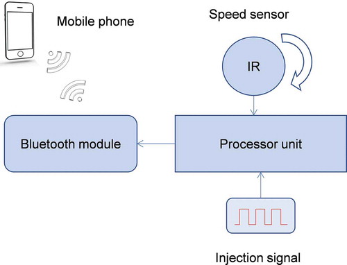
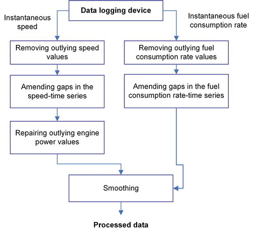
This study aims at developing the data logging device for measuring and storing the data of instantaneous speed and fuel consumption of MC. The device consists of three main parts including signal input unit, processing unit, and monitoring and storing unit. The input unit has two modules. The measuring module of instantaneous speed of MC, called a speed module, receives pulse signals from infrared sensor for vehicle speed measurement. The measuring module of instantaneous fuel consumption, called a fuel module, receives injection pulse signal for fuel consumption measurement. The processing unit was developed based on a microcontroller Atmega 2560 and other components such as voltage regulator, crystal oscillator, etc. In addition, the monitoring and storing unit, which consists of a Bluetooth module and a portable device, was also used for monitoring and storing measured data during on-road driving. The block principle of data logging device is presented in Figure 1.

Figure 1. Principle diagram of the data logging device

Principle of determining the instantaneous speed by infrared sensor

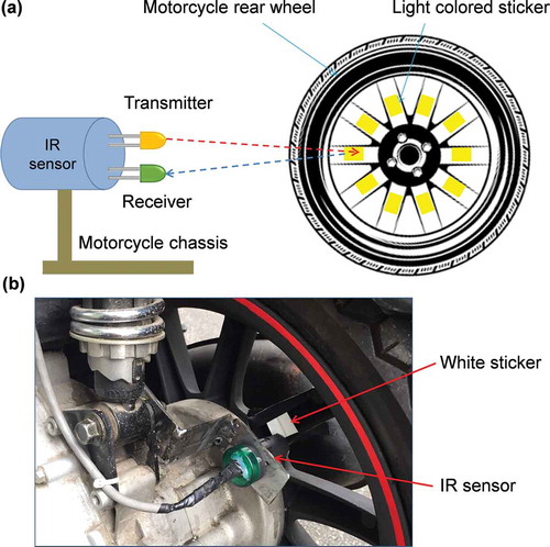
The instantaneous speed of MC is calculated indirectly through wheel radius and rotational speed. The rotational speed of the wheel is measured by an infrared sensor (IR) which is installed on the chassis of the MC. The IR sensor used in this study is a compact type and had fast detection speed. The schematic diagram of wheel rotational speed measurement is presented in Figure 2.

Figure 2. Schematic diagram of wheel rotational speed measurement (a) and the sensor installed on the test vehicle (b)

The instantaneous speed of test MC is calculated second by second following the Equation (1)(1) $V=\frac{7.2\times \pi \times R}{z\times \mathrm{\Delta }t}$(1) :

(1) $V=\frac{7.2\times \pi \times R}{z\times \mathrm{\Delta }t}$(1)

where V is the instantaneous speed of the MC (km/h), R is the wheel radius (m), z is the number of reflecting signal per revolution of wheel, and Δt is the average of time interval between two consecutive signals received from IR sensor in one second (s), called average period of pulse.

There are two methods of determining the wheel revolution, namely frequency and period method. The selection of method for rotational speed determination belongs to each application and the value of measured speed. In this study, the period method has been used to measure the rotational speed of the wheel. Because in actual operating condition of the test MC, sometime the MC is in stationary state so that the period method is selected for this purpose. The instantaneous speed of the MC was calculated from the average period of the pulse, which was basically determined following the flowchart as shown in Figure 3.

Figure 3. Flowchart of measuring instantaneous speed

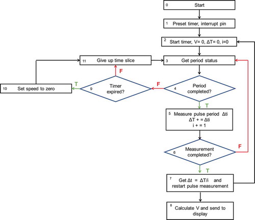
Figure 3 shows the programming flowchart of speed measurement by measuring the pulse period. As can be seen on the flowchart, the microcontroller presets the timer and interrupt pin (one interrupt pin for raising edge of reflected signal from IR sensor). During the operation, the microcontroller waits for a new raising interrupt. If the interruption occurs, the timer counter is started, and the microcontroller waits for the next occurrence of the interruption. If the next interruption occurs, the timer counter is stopped, and then the counted value is returned. The MC speed is calculated by taking into account the counted value, and finally, the calculated value is sent to the monitoring and storing device.

By using the period of pulse measuring method, the main problem is the detection of zero speed as the MC in stationary condition. To solve this problem, a logic flow on the left of the flowchart can be used. If the duration between two consecutive pulses is longer than an allowable value, the microcontroller would recognize that the wheel has been stopped. Particularly, the system has restarted the timer after each pulse completed, and if the next pulse is not received before the timer expires, it means that the MC is in idle mode.

Principle of determining the instantaneous fuel consumption rate (FR) from injection pulse

In this study, a simple but effective method was proposed to measure the instantaneous FR of MC. In the operation of the engine, the amount of fuel supplied to the engine is directly controlled through the injection pulse. The injection pulse width or injection duration is controlled by the electronic controller module (ECM). There is a strong correlation between injection pulse width and the injected amount of fuel. So as a result, measuring injection pulse width could be a quite simple way to determine actual fuel consumed by the engine. The method of measuring instantaneous fuel consumption is illustrated in Figure 4.

Figure 4. Principle of fuel consumption measurement

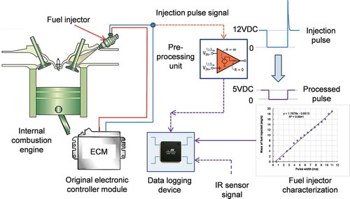
As shown in Figure 4, the data logging device receives the injection pulse commanded from the ECM as a digital input signal. By measuring the width of the pulse, the injected amount of fuel could be calculated. Measuring the actual injection pulse is a simple but effective method, which does not affect the engine operation because the injection pulse is remaining.

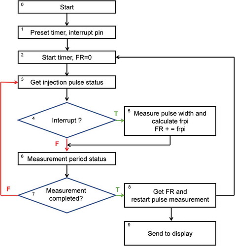
Figure 5 presents the programming flowchart for the measurement of fuel consumption in mg per second. As can be seen in Figure 5, the microcontroller presets the timer and interrupt pins (one for raising edge and one for falling edge of the injection pulse). During operation, if the interruption for falling edge occurs, the timer counter is started, and the second interruption of raising edge occurs, the timer counter is stopped, and the counted value is used to calculate the amount of fuel injected per one injection time (frpi, mg). The second-by-second fuel consumption (FR) is the summary of the total frpi in one measurement period of 1 second.

Figure 5. Flowchart of measuring instantaneous fuel consumption

Calculation of FR

The carbon balance method using a constant volume sampler (CVS) was used to validate the developed method for the measurement of the FR in this study. The details of the FR calculated from the developed method and the carbon balance method are presented as follows.

Proposed method using in the data logging device

In order to calculate the injected amount of fuel from the injection duration, it is necessary to determine the injector characteristics. The characteristics of the fuel injector represent the relationship between the injection duration and the injected amount of fuel. In this study, a laboratory test was carried out to measure the injected amount of fuel corresponding to the injection duration. The experimental diagram for the determination of the fuel characteristics is presented in Figure 6.

Figure 6. Experimental diagram for determining characteristics of injector

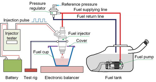
The test was conducted at laboratory condition with the average ambient temperature of 25°C and the atmospheric pressure of 101.3 kPa. The original fuel tank, fuel pump, and fuel line were used in the test as presented in Figure 6. As can be seen in the experimental diagram, injection pulse is commanded from an injection tester, which consists of a power supply source and pulse generator module. The injection tester allows users to adjust flexibly the injection pulse width and the number of injection time with injection frequency up to 10 Hz. During real life operation of the engine, there is an effect of the variation of vacuum pressure; therefore, in this study, the fuel pressure was maintained at a constant value of 3 bar by the pressure regulator installed on the supplying line. At each test mode, the number of injection time of 600 was set constantly, and injection duration was varied from 0 to 12 ms with interval of 0.65 ms.

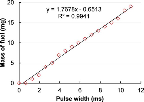
The testing result shows that there is a strong correlation between the injection duration of the injector and the fuel rate as described in Figure 7.

Figure 7. Relationship between the fuel rate and the injection duration

The FR is calculated from the amount of injected fuel in one second as shown in Equation (2)(2) $FR=\sum _{i=1}^n\left(1.7678\times PW-0.6513\right)$(2) :

(2) $FR=\sum _{i=1}^n\left(1.7678\times PW-0.6513\right)$(2)

where FR is the FR (mg/s), PW (pulse width) is the injection duration (ms), i is the injection time, and n is the number of injection time in one second.

In addition, during on-road operation, there is an effect of actual temperature; therefore, the actual fuel injected is determined by Equation (3)(3) $F{R}_{act}=\sum _{i=1}^n\left(1.7678\times PW-0.6513\right)\times k_T$(3) :

(3) $F{R}_{act}=\sum _{i=1}^n\left(1.7678\times PW-0.6513\right)\times k_T$(3)

where FR_act is the actual FR (mg/s), and k_T is the temperature correction factor.

The k_T factor, which is used to correct the actual density of fuel following the actual operation temperature, is determined by Equation (4)(4) $k_T=\frac{{\rho }_T}{{\rho }_{25}}$(4) :

(4) $k_T=\frac{{\rho }_T}{{\rho }_{25}}$(4)

where ρ_T and ρ₂₅ are the density of fuel at actual operation temperature and testing temperature of 25°C, respectively.

The correlations for fuel density and temperature are calculated using the tools based on ASTM D 1250-04.

Carbon balancer method

The carbon balance method is commonly used to calculate the FR based on the theory that the total mass of carbon element in consumed fuel is equal to that in exhaust gases. The instantaneous FR is calculated from the flow rate of CO₂, CO, and HC emission in exhaust gases from spark ignition engine as presented in Equation (5)(5) $FR=\frac{1}{C_F}\times \left(\frac{M_C}{{\alpha }_{exh}\times M_H+M_C}\right)\times m_{HC}\left(t\right)+\frac{M_C}{M_{CO}}\times m_{CO}\left(t\right)+\frac{M_C}{M_{C{O}_2}}\times m_{C{O}_2}\left(t\right)$(5) (Akita, Nakamura, and Adachi 2013), while the content of particulate matter is ignored:

(5) $FR=\frac{1}{C_F}\times \left(\frac{M_C}{{\alpha }_{exh}\times M_H+M_C}\right)\times m_{HC}\left(t\right)+\frac{M_C}{M_{CO}}\times m_{CO}\left(t\right)+\frac{M_C}{M_{C{O}_2}}\times m_{C{O}_2}\left(t\right)$(5)

where FR is the instantaneous FR at time t, mg/s; C_F is the mass fraction of carbon in fuel used, m_HC (t), m_CO (t), and m_CO2 (t) are the flow rate of HC, CO, and CO₂ components at time t, mg/s, respectively; M_H, M_C, M_CO, and M_CO2 are the molar mass for each component H, C, CO, and CO₂, respectively, g/mol, and α_exh is the average hydrogen-carbon atomic ratio for HC in exhaust gas, α_exh = 1.85 for gasoline (ECOSOC 2003).

In this study, the continuous mass flow rate of HC, CO, and CO₂ emissions was calculated from emission concentration by measuring diluted exhaust gas with the CVS system and emission analyzer devices.

Calculation of average fuel consumption

The average fuel consumption level for each trip is calculated based on the instantaneous speed and FR of this trip itself as presented in Equation (6)(6) ${\overline{FC}}_{km}=100\times \frac{{\sum }_{i=1}^{n}F{R}_i}{{\sum }_{i=1}^n\frac{v_i}{3600}}\times \frac{1}{{\rho }_{fuel}}$(6) :

(6) ${\overline{FC}}_{km}=100\times \frac{{\sum }_{i=1}^{n}F{R}_i}{{\sum }_{i=1}^n\frac{v_i}{3600}}\times \frac{1}{{\rho }_{fuel}}$(6)

where ${\overline{FC}}_{km}$ is the average fuel consumption level (L/100 km); n is the number of data points in the trip; FC_i is the instantaneous FR at the data point i (g/s); v_i is speed at the data point i (km/h), ρ_fuel is the density of fuel (g/L).

In addition, the average fuel consumption level also can be determined through the carbon balance method by Equation (7)(7) $FC=\frac{0.1154}{\rho }\times \left(0.866\times m_{HC}+0.429\times m_{CO}+0.273\times m_{C{O}_2}\right)$(7) :

(7) $FC=\frac{0.1154}{\rho }\times \left(0.866\times m_{HC}+0.429\times m_{CO}+0.273\times m_{C{O}_2}\right)$(7)

where FC is the fuel consumption in l/100 km; m_HC, m_CO, and m_CO2 are the measured emission of HC, CO, and CO₂ in g/km, respectively, and ρ is fuel density (kg/m³).

Connecting to the on-road data logging device

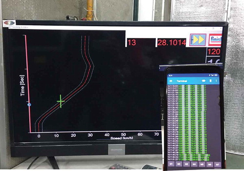
As explained above, the data logging device has been connected with a mobile phone through the Bluetooth module for continuous monitoring during on-road driving as well as storing measured data in real-time format. The monitoring device is a mobile phone, installed with a developed application based on Android Platform by MIT App Inventor. The mobile phone can connect to the Bluetooth module through the soft serial communication, so that it allows the processor unit to send the measured data to the phone for monitoring and storing without any delay. The picture of application installed mobile phone and the driver aid computer in laboratory test is shown in Figure 8.

Figure 8. The application installed mobile phone and the driver aid computer in laboratory test

Data preprocessing

Testing stationarity

The signal received from the data logging device includes the time series of instantaneous speed and FR with the time step of 1 second. Therefore, the stationarity of these time series has to be tested to make sure that the statistical properties of a process generating a time series do not change over time. It is necessary to use these time series in estimating trend, forecasting, and inferring causal relation because the mean and variance of the time series are constant over time (Gujarati 2009; Palachy 2019). In other words, testing the stationarity of time series before applying the noise reduction algorithms (e.g., smoothing and prediction) is very important. Therefore, the stationarity of time series of speed and FR are needed to be tested before they undergo the filtration process.

The instantaneous speed of the vehicle on the road, known as the time series, has been tested the stationarity in the study of Nguyen et al. (2019). Therefore, this study only tests the stationarity for the time series of the FR of vehicle. The Econometrics Toolbox™ of Matlab2017a was used to test the stationarity of the instantaneous FR series. The unit root test using the Augmented Dickey–Fuller (ADF) test was used to check the stationarity for this time series.

Designing the filtration process

The datasets including the second-by-second speed-time and the fuel consumption-time, which are collected from the data logging device, must be preprocessed to remove the random errors and reduce the effect of white noise. This step is necessary to prevent serious errors in calculating the time series of acceleration, fuel consumption, as well as the vehicle specific power (VSP) if available. In the range of high speed, any unsmoothed speed can lead to high deviation between the actual VSP as well as fuel consumption and the predicted ones (Smit 2013). Therefore, in this study, a filtration process for preprocessing the instantaneous speed and FR for the development of driving cycle or fuel consumption prediction models was proposed. Overall steps of filter process were arranged in increasing complexity order as presented in Figure 9. This arranging was also used efficiently in the study of Duran and Earleywine (2012). The designed filter aims to minimize noise while maintaining data integrity.

Figure 9. Flowchart of filtration process

Removing outliers

The first step of filtration process is removing the outlying speed and fuel consumption values in two datasets, including the speed and the fuel consumption series. The limits of speed and fuel consumption were set up to determine the outlying values. After that, a gap was created at the position of this outlier. The speed or fuel consumption value at this gap was found again by using the estimation algorithm of missing data, which was developed by Selesnick (2013) as presented in Equation (8)(8) $\hat{x}=S^{T}y+S_C^{T}v$(8) . The efficiency of estimating the missing data by this algorithm was demonstrated in the study of Nguyen et al. (2020), in which, the root mean square errors (RMSE) between the true data and the estimated data according to the Selesnick’s algorithm is smallest. The proposed algorithm by Selesnick is presented in Equation (8)(8) $\hat{x}=S^{T}y+S_C^{T}v$(8) (Selesnick 2013):

(8) $\hat{x}=S^{T}y+S_C^{T}v$(8)

where Suppose x is the signal involving missing data points which needs to be filled; then, $\hat{x}$is the estimated value for gaps in the vector x, S^T is the transpose of matrix S, in which S is the sampling matrix, $S_c^T$ is the transpose of matrix S_c, in which S_c is the complement matrix of S, y is the vector consisting of the available data, and v is the vector consisting of the samples to be determined.

Amending gaps in the speed-time and the FR-time series

In the second step of the filtration process, the filter was designed to detect and amend the gaps in the speed-time and the FR-time series. It is necessary to make sure that the time-series of speed as well as FR have the homogeneous time step of one second. First, the filter checks the time step between consecutive two data points in each dataset. If this time step is greater than one second, the filter would recognize a gap at this position. After that, the estimation algorithm of missing data developed by Selesnick as presented above was used to fill this gap.

Repairing outlying engine power values

In the third step of filter process, the remaining random errors in the speed profile would be continuously removed by searching for errors in the secondary dataset of instantaneous engine power. In which, the derivative with respect to time of the instantaneous speed, called the instantaneous acceleration, would be checked to ensure that the recorded speed matches expected engine power. Supposing the power train loss of 8%, the engine power is determined as follows (Bishop et al. 2016):

(9) $P=1.08\times m\times VSP$(9)

where P is the engine power (kW), m is the vehicle mass (tons), and VSP is the vehicle specific power (kW/ton). For MC, the VSP is calculated as follows (Duarte, Gonçalves, and Farias 2014; Jimenez-Palacios 1999; Son, Zhang, and Fujiwara 2012):

(10) $VSP=v\times \left(1.1\times a+9.81\times atan(sin(grade\right))+0.132)+3.02\times {10}^{-4}\times v^3$(10)

where v is the vehicle speed (m/s), a is the vehicle acceleration (m/s²), and grade is the grade of road (degree).

The instantaneous acceleration is calculated based on the speed change in each interval of time as presented in Equation (11)(11) $a=\frac{v_i-v_{i-1}}{Ts}$(11) :

(11) $a=\frac{v_i-v_{i-1}}{Ts}$(11)

where Ts is the time step (s), and v is the instantaneous speed (m/s).

The filter was designed to check the abnormal values in the secondary dataset calculated above and then correct the error of speed values at corresponding positions on the speed dataset. For this approach, if the value of engine power at any point is higher than the maximum engine power of the test vehicle, the engine power at that point is considered as the abnormal value. After that, the filter would delete the speed values at corresponding positions with the positions of these abnormal values to create gaps. Then, these gaps are filled using the algorithm of Selesnick (2013) as presented above.

Smooth final signals

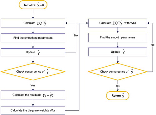
In the final step of the filtration process, the instantaneous speed and FR were smoothed to remove any underlying noise remained in these datasets. Smoothing is one of statistical smoothing techniques used commonly to reduce noise in the signal based on the past and future samples of the signal (Jun, Guensler, and Ogle 2006; Kowalski and Smyk 2018). In smoothing techniques, the Kalman filter is one of the most typical filtering techniques based on the use of the unsupervised filtering algorithm (Jun, Guensler, and Ogle 2006; Nguyen et al. 2019; Park et al. 2019). However, the Kalman filter requires users to correctly furnish the covariance matrixes of process noise (Q) and measurement noise (R). It is not easy for users to know the accuracy of noise information (Park et al. 2019). Therefore, in this study, another approach in smoothing data, which was developed by Garcia (2010), was used as the final step of filtration process. In the study of Garcia (2010), a fast robust smoothing, abbreviated r-smooth, based on the discrete cosine transform (DCT) was proposed to smooth robustly the data with equal space. Garcia used the following model to consider the noise signal y (12):

(12) $y=\hat{y}+\epsilon$(12)

where $\hat{y}$ is the signal which is supposed to be smooth, and ε is the Gaussian noise.

In the algorithm proposed by Garcia (2010), the y signal is smoothed based on finding the best estimate of $\hat{y}$ as demonstrated in Figure 10, in which DCT is the discrete cosine transform, and Wbs is the bisquare weight used to minimize or remove the effects of high leverage and outlying points. For more details on the algorithm and program code, the readers should refer to (Garcia 2010).

Figure 10. Flowchart of robust smoothing algorithm of data with missing values

In addition, determining the FR through measuring the pulse width of fuel injection can capture well the fuel supply cutoff phenomenon during abrupt deceleration. This causes the existence of zero fuel values in the collected FR profile. As such, the values are known as rare events. Therefore, smoothing the FR dataset could recognize these data points same as aberrant values and smooth them. So, in order to avoid losing the data points related to this phenomenon, the smoothed dataset returned the zero values at the positions that had been recognized appearing the abrupt deceleration based on the raw dataset, in which any data points with negative acceleration and zero fuel rate are recognized being fuel cutoff points.

All steps of data filtration process as presented in Figure 10 were performed on the Matlab2018a software.

Results and discussion

The effectiveness of data logging device as well as designed data filter are estimated in this section.

Stationarity test result

As mentioned above, the stationarity of speed-time series has been tested in the study of Nguyen et al. (2019). Therefore, only the time series of FR was tested for that purpose in this study using the ADF test. The obtained test result indicates that the time series of FR is the stationarity time series because the absolute value of the estimated τ value (|τ| = 5.931) is higher than the absolute value of 5% critical value (|τ_0.5| = 2.867) (Gujarati 2009). Therefore, both the speed-time series and FR-time series are the stationary time series. This creates the certainty of estimating missing data as well as smoothing and denoising in the preprocessing process for these datasets.

Data processing results

In order to clarify the effectiveness of the designed filter, the data logging device was used to collect the on-road driving data of the vehicle including the instantaneous speed and FR. The Vespa Liberty 3Vie motorcycle was used to install the sensors of data logging device. Petroleum A95, commercial fuel on the Vietnamese market, was used in the experiment. The specifications of the test motorcycle and engine are presented in Table 2.

Table 2. Specifications of the test motorcycle

Branch and model	Piaggio Liberty 3Vie
Engine	Single cylinder, 4 strokes, OHC 3 valves, Spark ignition
Model year	2013
Mileage	20,000 km
Displacement	149 cm^3
Bore x Stroke	62.2 × 48.6 mm
Compression ratio	11.1:1
Max power	8.60 kW/8,000 rpm
Max torque	11.20 Nm/6,250 rpm
Fuel system	Port fuel injection
Transmission system	CVT
After-treatment	Three-way catalyst

Filter inputs

By driving the test vehicle connected to the data logging device on the urban road in Hanoi, the real-world driving data of 25 trips were used to estimate the effectiveness of the proposed filter. In addition, several limit parameters related to the test vehicle characteristics and the urban speed limit in Hanoi were also used as presented in Table 3.

Table 3. Filtration limits

Parameters	Limit
Speed limit	60 km/h
Max engine power	8.60 kW
Max fuel consumption rate at the speed limit of 60 km/h	250 mg/s^(*)

Notes. The limit value of 250 mg/s was inherited from laboratory test in the study of Le (2016).

Evaluation of the filter effectiveness

Analyzing the strictness of designed filter

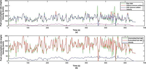
First of all, the effectiveness of the designed filter was reflected through the logic of processing steps. As mentioned above, all outlying data points were removed to create gaps; after that, the estimation missing data algorithm of Selesnick (2013) was used to fill these gaps. This approach was estimated well in the study of Nguyen et al. (2020). As illustrated in Figure 11, any data points higher than the established limit values (e.g., 60 km/h for speed and 250 mg/s for the FR) were detected and replaced by new values. Removing these outliers is necessary to improve the effectiveness of the final smooth step. As can be seen in Figure 12a, the FR profile, smoothed without removing outliers before, still contain values over the limit of 250 mg/s (e.g., the FR of 286.8 mg/s at the time of 244s). This is not suitable with the specifications of the test vehicle, whereas these data points disappear in case that the dataset has been removed outliers before being smoothed. This can be explained by the fact that the appearance of abnormal high value can mislead the estimation in the smoothing technique. However, if removing outliers only without the final smooth step, removing noise is also not sufficient as illustrated in Figure 12b. According to Figure 12b, the unsmoothed FR data oscillate strongly even when the speed oscillation is small. Furthermore, the dataset related to the unsmoothed FR contains the zero values while the speed values at present, near past, and future are not equal to zero (e.g., at time of 466 s and 551 s). In other words, the filter was designed closely with arranging steps in the order of increasing complexity.

Figure 11. Illustration of detecting and repairing the outlying data

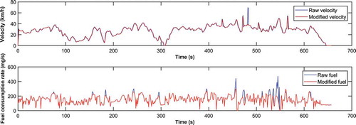
Figure 12. Illustration of the filter effectiveness. (a) Comparison collected data between with and without removing outliers before smoothing. (b) Comparison collected data between with and without final smoothing

Comparing smooth methods

The efficiency of the designed filter was also estimated by comparing with other smoothing methods. As mentioned above, the robust smoothing technique developed by Garcia (2010) was used to smooth noise in this study. The r-smooth’s efficiency was estimated through comparing with the Savitzky-Golay and Kalman filters. These filters were used commonly in many recent studies (Duran and Earleywine 2012; Eliasson 2014; Gomez-Gil et al. 2013; Jun, Guensler, and Ogle 2006; Kowalski and Smyk 2018) (see Figure 13).

Figure 13. Comparison between different filter methods

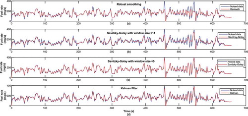
As shown in Figure 13d, the raw and denoised data seem to overlap, including outliers. It implies that the Kalman filter failed to denoise in the FR data because the process and measurement noise covariance were not determined exactly. In fact, determining these noises is not easy for users (Park et al. 2019). Therefore, the Kalman filter has not been recommended for using in the applied studies without determining exactly the process and measurement noise covariance. For the Savitzky-Golay filter, as can be seen from Figure 13b–c, its efficiency depends strongly on the chosen window size as well as the decided order of polynomial regression. Even when the profile of smoothed data using the Savitzky-Golay filter is quite similar to that obtained by using the r-smooth filter (Figure 13a–b), the outliers still could not be removed (e.g., at time 546 s, the FR estimated according to the Savitzky-Golay filter and the r-smooth are 345.9 mg/s and 188.0 mg/s, respectively). In fact, it is difficult to decide the window size as well as the order for polynomial regression. Therefore, with the Savitzky-Golay filter it is also difficult to obtain high efficiency. After all things have been explored above, it can be concluded that the r-smooth filter not only achieves the high efficiency of denoise but also applies easily.

In addition, the effectiveness of the designed filter is also estimated through the results of processing data as depicted in the following analysis.

Ratio of random errors

The ratio of random errors related to outliers of speed and fuel as well as gaps of the time series of speed and FR are presented in Table 4.

Table 4. Filtration results

Filter name	Mean (%)	Median (%)	Standard deviation (%)
Outlying speed values	1.6	0	3.3
Outlying power values^(*)	0.2	0	0.5
Outlying fuel values	2.4	0.5	3.2
Speed gaps	0	0	0
Fuel gaps	0	0	0

Notes. The values in this table were determined based on the 25 independent results of data preprocessing obtained through the preprocessing of 25 traveling datasets; ^(*) the percentage of outlying power related to the fail speed values.

As can be seen from Table 4, on average, approximately 1.8% (sum of 1.6% and 0.2%) and 2.4% of the original speed and FR datasets, respectively, were taken in some different levels of the filter excepting the final smoothing step. Among them, the percentage of error related to the outlying fuel values is the highest, approximately 2.4%. The second highest ratio is the error related to the outlying speed values, approximately 1.6%. This ratio is higher than that related to outlying speed of 0.0015% in the speed profile collected using the GPS technique as presented in (Nguyen et al. 2019). However, random errors in the speed profile collected by the developed device is 1.8%, which is approximately 3.9 times smaller than that collected using GPS. In addition, there is not any error related to signal gaps. This implies that using sensors directly installed on the vehicle is successful in logging the on-road operation data, second-by-second. In other words, the data logging device can capture the second-by-second real-world driving data well.

Moreover, as can be seen from Table 4, the percentage of error related to the outlying power values is not equal to zero. This indicates that checking the misleading speed values based on checking the engine power is necessary, even when the outlying speed values have been removed before smoothing. A misleading speed value, not including the outlying value, could make the engine power value unsuitable with the engine performance level. Because the engine power is calculated based on the speed and the derivative speed with respect to time (see Equations (10(10) $VSP=v\times \left(1.1\times a+9.81\times atan(sin(grade\right))+0.132)+3.02\times {10}^{-4}\times v^3$(10) , 11(11) $a=\frac{v_i-v_{i-1}}{Ts}$(11) )). In other words, the filter was designed closely based on the logic of increasing complexity.

Comparison between raw and processed data

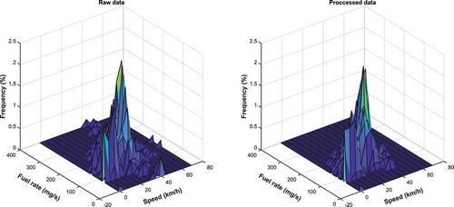
The effectiveness of the designed filter was estimated through comparison between the raw data and the processed data (see Table 5 and Figure 14).

Table 5. Comparison of the raw and processed data

Parameters	Raw data			Processed data
	Average	Median	Standard deviation	Average	Median	Standard deviation
Maximum speed (km/h)	181.3	42.4	257.3	39.7	39.8	10.26
Average speed (km/h)	23.1	20.7	8.5	20	18.2	5.2
Standard deviation of speed (km/h)	21.7	10.7	24.2	9.9	9.8	2.1
Maximum engine power (kW)	963.4	2.9	1728.1	3.6	2.3	3.3
Maximum fuel consumption rate (mg/s)	333.1	289.2	128.2	217.8	221.6	29.9
Average fuel consumption rate (mg/s)	123.7	115.3	21.3	122.7	114.7	20.1
Average fuel consumption (l/100 km)	3.1	-	-	2.7	-	-

Figure 14. Comparison of the frequency distribution of the speed–fuel consumption rate

The values in Table 5 were determined based on the 25 independent datasets which were obtained from the preprocessing of 25 input travel datasets.

As presented in Table 5, all the descriptive statistics of parameters related to input data in the raw data are higher than those in the processed data because there are outlying values in the raw data (see Figure 14). In fact, the percentage of outlying data is not high (1.6% and 2.4% for the speed and FR, respectively), but the values of these outliers are high, and this is the significant difference. In addition, the largest difference between the raw data and processed data is detected for the maximum engine power even when the percentage of outlying power values is the smallest, around 0.2% (see Table 4). The maximum power of engine in the raw data is 112 times exceeding the limit of maximum engine power. This reconfirms that checking the derivative of speed with respect to time based on the evaluation of the confidence of the engine power is necessary. Furthermore, results in Figure 14 indicate that the frequency distribution of the speed-FR of the raw data and processed data is quite homologous, except several outliers. This implies that the filter was well designed to remove outliers as well as noise in the raw data while retaining the integrity of the original data profile. Furthermore, the efficiency of designed filter has also been confirmed through its ability to reflect exactly the actual fuel economy of test vehicle. The average fuel economy of the test MC, which is calculated based on the processed data (2.7 L/100 km), is close to the result obtained by the carbon balance method (2.86 L/100 km) (the content of experiment activity is discussed next).

Evaluating the accuracy of the developed data logging device

To assess the accuracy of the developed device, a verification measurement was performed for the test MC on the motorcycle chassis dynamometer AVL CD20” at steady state and following the World Motorcycle Test Cycle (WMTC) driving cycle. The instantaneous speed measured by the developed device emission components was used to compare to the one measured by the chassis dynamometer. Meanwhile, the measured FR was compared to the calculated one from emission components which were measured by the CVS system. The experiment was conducted in the Research Center for Engines, Fuels, and Emissions, School of Transportation Engineering, Hanoi University of Science and Technology, Hanoi, Vietnam.

Evaluating the ability of instantaneous speed measurement

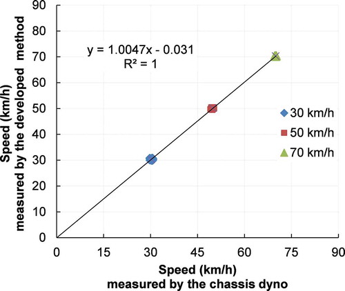
At steady state

The test MC was operated at steady state to validate the measured speed value by the developed data collection system. The MC ran at constant speeds of 30 km/h, 50 km/h, and 70 km/h. The result on Figure 15 shows that there is a deviation between the speed results which were measured by difference methods. The average deviation is approximately 0.35%. The difference can be explained by the fact that the process of calculating vehicle speed based on the wheel radius ignored the change of the wheel radius during the operation process. In addition, the actual radius of wheel was changed due to the total mass of the test MC including the MC’s load itself and the driver. However, the difference is relatively small.

Figure 15. The correlation of measured speed with the chassis dyno

At transient state

The experiment in transient mode was conducted to evaluate the ability of the developed device in capturing the speed of the test MC. The test MC was driven following the transient driving cycle WMTC. The speed profiles which are determined according to the chassis dynamometer and the developed device, as presented in Figure 16.

Figure 16. Comparison of speed measured by developed device and chassis dynamometer

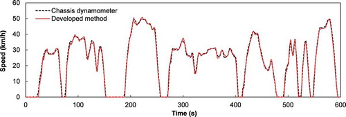
As can be seen in Figure 16, there is a very strong correlation between the two datasets; the biggest deviation between these two datasets is less than 3.5% at the moment where the MC is accelerated or braked. The deviation could be the result of the slip between the wheel and the roller. Therefore, the developed device is successful in recording the instantaneous speed of vehicle.

Evaluating the ability of FR measurement

At steady state

Figure 17 illustrates the correlation of two datasets of average FR which is determined according to the proposed method and the carbon balance method using the CVS system. The result of FR measured by the developed method in this section is the corrected result that has taken the temperature correction factors into account.

Figure 17. The correlation between two datasets of fuel consumption rate

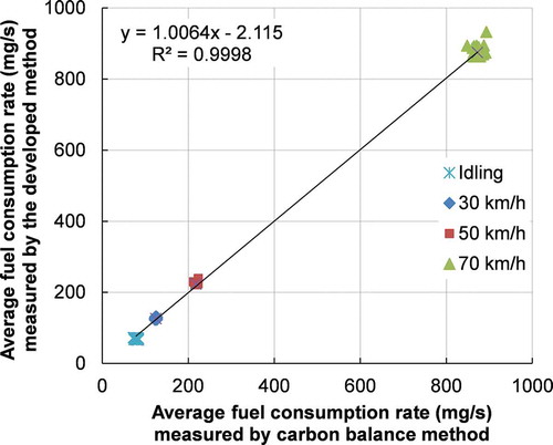
The average value of three repeated measurements under the steady state, in which the duration of each measurement is 5 minutes, is used to analyze the correlation above. As can be seen in Figure 16, there is a high correlation between two datasets (R² > 0.99). The average FR measured by the developed device is slightly different from the one measured by the carbon balance method, 0.25% at 70 km/h, 2.56% at 50 km/h, and 0.92% at 30 km/h, respectively. However, at idling speed, the difference is 11.6%. This can be explained by the fact that the variation of intake manifold pressure in idling condition is significant. As a result, the fuel pressure regulator could not maintain the constant value of fuel pressure. Consequently, the difference pressure of three bars on the fuel injector could not be maintained resulting in reducing the accuracy of calculated fuel by the developed method.

At transient state

For the CVS system, emission components were analyzed from the diluted exhaust gas, so that, there was a time lag among the measured concentration of emission components and the MC speed. As a result, the profile of FR which was determined using the carbon balance method has low response to the speed signal of test MC. In contrast, the developed method has high response to the speed signal of the test MC. The reason for this can be the direct determination of the instantaneous FR based on the injection pulse width proposed by this study. Figure 18 shows that the profile of FR measured by the proposed method has quick response, which agrees well with the speed of test MC. This could be seen clearly on the initial seconds of the driving cycle (11th second) when the test MC was just accelerated from idling mode. In other words, the proposed method is suitable for the on-road fuel consumption measurement test.

Figure 18. The comparison of the signal update ability of the instantaneous fuel consumption rate between two methods

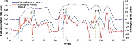
The time lag value (τ) depends on the length of the exhaust sampling system. In this test, we observed that the time lag varied from 3 to 5 s. Therefore, in order to have a good comparison of instantaneous FR measured by the two methods, the profile of FR measured by the carbon balance method was shifted to the left about 4 s to achieve best fit between the profiles of FR measured by developed method and measured speed profile.

As shown in Figure 19, after the profile of FR measured by the carbon balance method was treated the time delay of 4 s, the correlation of measurements of FR between two methods has a good agreement and high response to the speed profile.

Figure 19. The correlation of measurements of fuel consumption rate between two methods

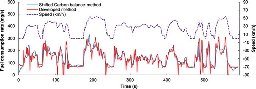
In addition, the advantage of the proposed method is observed clearly at the moment after starting the engine (the initial seconds) or during rapid brake condition around 120 s, 240 s, and 570 s, where the injected amount of fuel is minimized. For example, when the MC was braked rapidly around the 240th second to idling mode, the fuel consumption measured by carbon balance method takes approximately 10 s more to acchive the idling value. Meanwhile, the fuel consumption measured by the developed method shows a rapid variation at these points and gains the idling value in a shorter time.

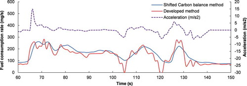
The experiment result shown in Figure 20 is the expanded view of fuel consumption measurement and MC acceleration results during a phase of WMTC driving cycle from the 60th to 150th second. The result shows that the fuel consumption rate, which is calculated by this developed method, is good corresponding to the MC acceleration profile. Specifically, around the 63th to 67th second, as the throttle is opened rapidly to accelerate from idling condition, there is a correlation between fuel rate and acceleration profile. However, the measured result calculated by the carbon balance method shows a slower response, especially at points (seconds 105 and 121) that the MC brakes rapidly. Around these points, the injected amount of fuel is small because the EMC commands a short duration of pulse to cut down supplying fuel. However, the response of fuel rate measured by the carbon balance method is later and slower than that of the developed method. The reason can be specified as there is a delay of transport in exhaust gas sampling. The emission level measured by the CVS system seems to be affected by the slow response at real-time measurements.

Figure 20. Example of measurement of real time fuel consumption with rapid acceleration and brake

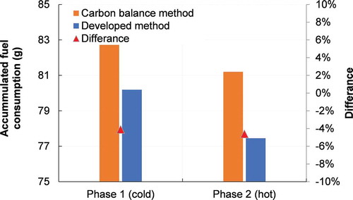
Figure 21 shows the accumulated fuel consumption during each phase of the WMTC driving cycle. The first phase of the driving cycle (second 0–600th) is called the cold phase because at the moment of starting the cycle, the engine starts from ambient temperature. The second phase (600–1,200 s) is the hot phase. For the first phase, the difference of accumulated fuel consumptions between the two methods is remarkable. The l value measured by the developed method is approximately 4.10% lower that monitored by carbon balance one. Moreover, for the hot phase, as the engine temperature is high enough, the accumulated fuel consumption reduces to 2.89% and 3.42% in comparison to ones measured in the cold phase by the developed method and carbon balance method, respectively. In addition, there is a difference in accumulated fuel consumption measured by the two methods, approximately 4.62%. In general, following a transient operation condition, accumulated fuel consumption measured by the developed method is 4.35% averagely lower than the actual fuel consumption. Table 6 presents the summary of measured emission and fuel consumption by two methods.

Table 6. The summary of measured emission and fuel consumption by two methods

Phase	Accumulated emission (g)			Accumulated Fuel consumption (g)		Difference
	CO	CO2	HC	Carbon balance method	Developed method
Cold (0–600s)	5.382	293.856	1.257	83.62	80.19	−4.10%
Hot (600–1,200s)	1.212	294.535	0.314	81.20	77.45	−4.62%
Difference	−7.48%	0.23%	−75.02%	−2.89%	−3.42%

Figure 21. Comparison of accumulated fuel consumption measured by two methods

The average fuel consumption of 2.7 L/100 km of the test MC is calculated based on the processed data as shown in Equation (6)(6) ${\overline{FC}}_{km}=100\times \frac{{\sum }_{i=1}^{n}F{R}_i}{{\sum }_{i=1}^n\frac{v_i}{3600}}\times \frac{1}{{\rho }_{fuel}}$(6) . This value is close to the value obtained by carbon balance method of 2.86 L/100 km, which is calculated by Equation (7)(7) $FC=\frac{0.1154}{\rho }\times \left(0.866\times m_{HC}+0.429\times m_{CO}+0.273\times m_{C{O}_2}\right)$(7) .

Based on the explanation and analysis above, with the advantage of high response ability, the developed method can be considered to have a possibility as a more precise method for transient fuel consumption measurement.

Conclusion

In this study, the data logging device has been developed and evaluated following laboratory conditions. At steady state, the average deviation between speeds measured by the chassis and the data logging device is approximately 0.35%. At transient state, the biggest deviation between these two datasets varies from 1.7% to 3.5%. The average FR measured by the developed device is slightly different from the one measured by the carbon balance method. The differences are 0.25% at 70 km/h, 2.56% at 50 km/h, and 0.92% at 30 km/h, respectively. Under the transient operation condition, on average, the accumulated fuel consumption measured by the developed method is 4.35% lower than the actual fuel consumption.

In addition, a filter was designed to remove noise in the dataset collected using the data logging device. The filter was designed based on the logic of increasing complexity, including removing outliers and final smooth. The random errors in the speed and the FR profiles were detected and replaced; the percentage of these errors is 1.8% and 2.4%, respectively. The developed data logging device in combination with the designed filter is more feasible and higher quality in collecting the on-road driving characteristics of MC, which consists of the instantaneous FR and speed. The developed method for the measurement of instantaneous fuel consumption can be considered to have a possibility as a more precise method for the measurement of transient fuel consumption. The data logging device and the filter which were developed in this study are effective tools for future studies relating to the fuel consumption and emission of MC on the road.

Disclosure statement

No potential conflict of interest was reported by the authors.

Additional information

Notes on contributors

Khanh Nguyen Duc

Khanh Nguyen Duc is a lecturer of Department of Internal Combustion Engine, the School of Transportation Engineering, Hanoi University of Science and Technology (HUST). His research direction is related to controlling, automation on internal combustion engines; the use of alternative fuels such as natural gas, biogas in internal combustion engine; and improvement and conversion of engine using conventional fuel to alternative ones.

Yen-Lien T. Nguyen

Yen-Lien T. Nguyen is Ph.D. and lecturer at the Faculty of Environment and Transport Safety, University of Transport and Communications. Her research experiences and tendencies focus on the simulation of vehicle emission, typical driving cycle development and the estimation of the potential of co-benefits of climate, air quality and health in transport sector.

Tien Nguyen Duy

Tien Nguyen Duy is a lecturer of Department of Internal Combustion Engine, the School of Transportation Engineering, Hanoi University of Science and Technology (HUST). His research direction is related to automation on internal combustion engines, vehicle emission, driving cycle development.

Trung-Dung Nghiem

Trung-Dung Nghiem is an Associate Professor and the former Dean of the Institute of Environmental Science and Technology (INEST), Hanoi University of Technology (HUST). His working experience is related to air pollution and environmental chemistry.

Anh-Tuan Le

Anh-Tuan Le is a Professor and Dean of the School of Transportation Engineering, Hanoi University of Technology (HUST). His research experiences and tendencies focus on alternative fuels; mixture formation and combustion in IC Engines; fuel consumption improvement methods; vehicle emission measurements and reduction.

Tuyen Pham Huu

Tuyen Pham Huu is an Associate Professor and Director of the Research Center for Engines, Fuels and Emissions, School of Transportation Engineering, Hanoi University of Science and Technology. His research experiences and tendencies focus on fuel and emission from vehicle.

References

- Akita, M., H. Nakamura, and M. Adachi. 2013. In-situ real-time fuel consumption measurement using raw exhaust flow meter and Zirconia AFR sensor. SAE Int. J. Commer. Veh. 6 (1):183–89. doi:10.4271/2013-01-1058.
- Bifulco, G. N., F. Galante, L. Pariota, and M. R. Spena. 2015. A linear model for the estimation of fuel consumption and the impact evaluation of advanced driving assistance systems. Sustainability 7 (10):14326–43. doi:10.3390/su71014326.
- Bishop, J. D., M. E. Stettler, N. Molden, and A. M. Boies. 2016. Engine maps of fuel use and emissions from transient driving cycles. Appl. Energy 183:202–17. doi:10.1016/j.apenergy.2016.08.175.
- Chen, K., W. Wang, H. Chen, C. Lin, H. Hsu, J. Kao, and M. Hu. 2003. Motorcycle emissions and fuel consumption in urban and rural driving conditions. Sci. Tot. Environ. 312 (1–3):113–22. doi:10.1016/S0048-9697(03)00196-7.
- Duarte, G. O., G. A. Gonçalves, and T. L. Farias. 2014. A methodology to estimate real-world vehicle fuel use and emissions based on certification cycle data. Procedia-Soc. Behav. Sci. 111:702–10. doi:10.1016/j.sbspro.2014.01.104.
- Duran, A., and M. Earleywine. 2012. GPS data filtration method for drive cycle analysis applications. SAE 2012 World Congress, National Renewable Energy Lab (NREL), Golden, CO, Vol. 1, No. NREL/CP-5400-53865.
- ECOSOC. 2003. Worldwide harmonised motorcycle emissions certification procedure. Accessed November 20, 2019. https://www.unece.org/fileadmin/DAM/trans/doc/2003/wp29grpe/TRANS-WP29-GRPE-46-inf15e.pdf.
- Eliasson, M. 2014. A Kalman filter approach to reduce position error for pedestrian applications in areas of bad GPS reception. Sweden: Department of Computing Science, Umeå University.
- Ferreira, H., C. M. Rodrigues, and C. Pinho. 2019. Impact of road geometry on vehicle energy consumption and CO2 emissions: An energy-efficiency rating methodology. Energies 13 (1):2–27. doi:10.3390/en13010119.
- Franco, V., M. Kousoulidou, M. Muntean, L. Ntziachristos, S. Hausberger, and P. Dilara. 2013. Road vehicle emission factors development: A review. Atmos. Environ. 70:84–97. doi:10.1016/j.atmosenv.2013.01.006.
- Garcia, D. 2010. Robust smoothing of gridded data in one and higher dimensions with missing values. Comput. Stat. Data Anal. 54 (4):1167–78. doi:10.1016/j.csda.2009.09.020.
- Giraldo, M., and J. I. Huertas. 2019. Real emissions, driving patterns and fuel consumption of in-use diesel buses operating at high altitude. Transp. Res. Part D: Transp. Environ. 77:21–36. doi:10.1016/j.trd.2019.10.004.
- Gomez-Gil, J., R. Ruiz-Gonzalez, S. Alonso-Garcia, and F. J. Gomez-Gil. 2013. A Kalman filter implementation for precision improvement in low-cost GPS positioning of tractors. Sens. Transducers 13 (11):15307–23. doi:10.3390/s131115307.
- Gujarati, D. N. 2009. Basic econometrics. 4th ed. New York: The McGraw-Hill.
- Hirota, K., and S. Kashima. 2020. How are automobile fuel quality standards guaranteed? Evidence from Indonesia, Malaysia and Vietnam. Transp. Res. Interdiscip. Perspect. 100089. doi:10.1016/j.trip.2019.100089.
- Jimenez-Palacios, J. L. 1999. Understanding and quantifying motor vehicle emissions with vehicle specific power and TILDAS remote sensing. PhD thesis, Massachusetts Institute of Technology, Cambridge.
- Jun, J., R. Guensler, and J. Ogle. 2006. Smoothing methods designed to minimize the impact of GPS random error on travel distance, speed, and acceleration profile estimates. Transp. Res. Rec.: J. Transp. Res. Board 1972:141–50. doi:10.3141/1972-19.
- Kan, Z., L. Tang, M.-P. Kwan, and X. Zhang. 2018. Estimating vehicle fuel consumption and emissions using GPS big data. Int. J. Environ. Res. Public Health 15 (4):566. doi:10.3390/ijerph15040566.
- Kowalski, P., and R. Smyk. 2018. Review and comparison of smoothing algorithms for one-dimensional data noise reduction. 2018 International Interdisciplinary PhD Workshop (IIPhDW), IEEE. doi:10.1109/IIPHDW.2018.8388373.
- Le, A. T. 2016. Principle investigator of a national research project entitled “Hydrogen rich gas production by catalytic reforming of gasoline to supply to the spark ignition engines aiming higher engine efficiency and emission reduction” coded KC.05.24/11-15.
- Le, A.-T., M. T. Pham, T. T. Nguyen, and D. V. Nguyen. 2013. Measurements of emission factors and fuel consumption for motocycles on a Chassis Dynamometer based on a localized driving cycle. ASEAN Eng. J. Part C 1 (1):73–85.
- Ligterink, N. E., and A. R. Eijk. 2014. Update analysis of real-world fuel consumption of business passenger cars based on Travelcard Nederland fuelpass data. Dutch Ministry of Infrastructure and Environment, TNO report.
- Lin, C., X. Zhou, D. Wu, and B. Gong. 2019. Estimation of emissions at signalized intersections using an improved MOVES model with GPS data. Int. J. Environ. Res. Public Health 16 (19):3647. doi:10.3390/ijerph16193647.
- Lipar, P., I. Strnad, M. Česnik, and T. Maher. 2016. Development of urban driving cycle with GPS data post processing. Promet – Traffic Transp. 28 (4):353–64. doi:10.7307/ptt.v28i4.1916.
- Nguyen, Y.-L. T., N.-D. Bui, T.-D. Nghiem, and A.-T. Le. 2020. GPS data processing for driving cycle development in Hanoi, Vietnam. J. Eng. Sci. Technol. 15 (2):1429–40.
- Nguyen, Y.-L. T., T.-D. Nghiem, A.-T. Le, and N.-D. Bui. 2019. Development of the typical driving cycle for buses in Hanoi, Vietnam. J. Air Waste Manage. Assoc. 69 (4):423–37. doi:10.1080/10962247.2018.1543736.
- Ogundare, J. O. 2016. Precision surveying: The principles and geomatics practice. Hoboken, NJ: John Wiley & Sons, Inc.
- Palachy, S. 2019. Stationarity in time series analysis: A review of the concept and types of stationarity. Accessed March 12, 2020. https://towardsdatascience.com/stationarity-in-time-series-analysis-90c94f27322.
- Park, S., M.-S. Gil, H. Im, and Y.-S. Moon. 2019. Measurement noise recommendation for efficient kalman filtering over a large amount of sensor data. Sensors 19 (5):1168. doi:10.3390/s19051168.
- Pathak, S. K., V. Sood, Y. Singh, and S. Channiwala. 2016. Real world vehicle emissions: Their correlation with driving parameters. Transp. Res. Part D: Transp. Environ. 44:157–76. doi:10.1016/j.trd.2016.02.001.
- Saerens, B., H. Rakha, K. Ahn, and E. Van Den Bulck. 2013. Assessment of alternative polynomial fuel consumption models for use in intelligent transportation systems applications. J. Intell. Transp. Syst. 17 (4):294–303. doi:10.1080/15472450.2013.764801.
- Satiennam, T., A. Seedam, T. Radpukdee, W. Satiennam, W. Pasangtiyo, and Y. Hashino. 2017. Development of on-road exhaust emission and fuel consumption models for motorcycles and application through traffic microsimulation. J. Adv. Transp. 2017. doi:10.1155/2017/3958967.
- Seedam, A., T. Satiennam, T. Radpukdee, and W. Satiennam. 2015. Development of onboard measurement system measuring driving pattern and exhaust emissions of motorcycle and its application in Khon Kaen city. IATSS Res. 39 (1):79–85. doi:10.1016/j.iatssr.2015.05.003.
- Selesnick, I. 2013. Least squares with examples in signal processing. Accessed April 21, 2017. https://cnx.org/contents/XRPKcVgh@1/Least-Squares-with-Examples-in-Signal-Processing.
- Singh, P., and S. Singh. 2014. Efficiency of different filters in removing noise from GPS data. Int. J. Sci. Res. (IJSR) 3 (6):603–07.
- Smit, R. 2013. Development and performance of a new vehicle emissions and fuel consumption software (PΔP) with a high resolution in time and space. Atmos. Pollut. Res. 4 (3):336–45. doi:10.5094/APR.2013.038.
- Son, L. A., J. Zhang, and A. Fujiwara. 2012. The MATLAB toolbox for GPS data to calculate motorcycle emission in Hanoi - Vietnam. Int. Conf. Environ. Energy Biotechnol. Singapore 33:1–6.
- Song, Y.-Y., E.-J. Yao, T. Zuo, and Z.-F. Lang. 2013. Emissions and fuel consumption modeling for evaluating environmental effectiveness of ITS strategies. Discrete Dyn. Nat. Soc. 2013:1–9. doi:10.1155/2013/581945.
- Tong, H., W. Hung, and C. Cheung. 2000. On-road motor vehicle emissions and fuel consumption in urban driving conditions. J. Air Waste Manage. Assoc. 50 (4):543–54. doi:10.1080/10473289.2000.10464041.
- Tsai, J.-H., H.-L. Chiang, Y.-C. Hsu, B.-J. Peng, and R.-F. Hung. 2005. Development of a local real world driving cycle for motorcycles for emission factor measurements. Atmos. Environ. 39 (35):6631–41. doi:10.1016/j.atmosenv.2005.07.040.
- Tzeng, G.-H., and -J.-J. Chen. 1998. Developing a Taipei motorcycle driving cycle for emissions and fuel economy. Transp. Res. Part D: Transp. Environ. 3 (1):19–27. doi:10.1016/s1361-9209(97)00008-4.
- Wang, H., L. Fu, Y. Zhou, and H. Li. 2008. Modelling of the fuel consumption for passenger cars regarding driving characteristics. Transp. Res. Part D: Transp. Environ. 13 (7):479–82. doi:10.1016/j.trd.2008.09.002.