Global emissions of NH₃, NO_x, and N₂O from biomass burning and the impact of climate change

ABSTRACT

Emissions of ammonia (NH₃), oxides of nitrogen (NO_x; NO +NO₂), and nitrous oxide (N₂O) from biomass burning were quantified on a global scale for 2001 to 2015. On average biomass burning emissions at a global scale over the period were as follows: 4.53 ± 0.51 Tg NH₃ year⁻¹, 14.65 ± 1.60 Tg NO_x year⁻¹, and 0.97 ± 0.11 Tg N₂O year⁻¹. Emissions were comparable to other emissions databases. Statistical regression models were developed to project NH₃, NO_x, and N₂O emissions from biomass burning as a function of burn area. Two future climate scenarios (RCP 4.5 and RCP 8.5) were analyzed for 2050–2055 (“mid-century”) and 2090–2095 (“end of century”). Under the assumptions made in this study, the results indicate emissions of all species are projected to increase under both the RCP 4.5 and RCP 8.5 climate scenarios.

Implications: This manuscript quantifies emissions of NH₃, NO_x, and N₂O on a global scale from biomass burning from 2001–2015 then creates regression models to predict emissions based on climate change. Because reactive nitrogen emissions have such an important role in the global nitrogen cycle, changes in these emissions could lead to a number of health and environmental impacts.

Introduction

Nitrogen is essential to all life forms; however, excess emissions of nitrogen compounds can have detrimental impacts on human health and the environment (Battye, Aneja, and Schlesinger 2017). For example, atmospheric deposition of major reactive nitrogen species can lead to a decrease in biological diversity, soil acidification, and eutrophication of lakes and coastal zones (Erisman et al. 2013; Galloway et al. 2004; Holtgrieve et al. 2011). These specific nitrogen gases also have a negative impact on air quality. For example, oxides of nitrogen (NO_x) can increase tropospheric ozone (O₃) formation, nitrous oxide (N₂O) is an important greenhouse gas, and ammonia (NH₃) can lead to the formation of fine particulate matter (PM_2.5) (Baek and Aneja 2004; Baek, Aneja, and Tong 2004; Chen et al. 2014). There are many adverse health effects associated with exposure to elevated concentrations of ozone and fine particulate matter, such as chronic bronchitis, aggravated asthma, irregular heartbeat, other cardiovascular and respiratory problems, and even death (Lelieveld et al. 2015; Pope and Dockery 2006; Pope, Ezzati, and Dockery 2009). PM_2.5 is also associated with several environmental impacts, such as reduced visibility and changes in the earth’s radiational balance (Behera and Sharma 2010; Fan et al. 2005; Heald et al. 2012; Wang et al. 2012). Increased emissions of these specific nitrogen species can impact climate change as well as human health and welfare (Davidson et al. 2011; Galloway et al. 2004; Gruber and Galloway 2008).

Although biomass burning is not the most prominent source of these specific nitrogen species in the atmosphere, there is evidence that biomass burning contributes significantly to ambient concentrations of NH₃, NO_x, and N₂O (Crutzen et al. 1979; Lobert et al. 1990). Emissions of these species come from nitrogen in the fuel, and the species released are dependent upon flame temperature (Roberts et al. 2020). The strength and frequency of fires are not only controlled by the properties of the fuel, human influence, and geography, but also by weather and climate (Liu, Stanturf, and Goodrick 2010; Pyne, Andrews, and Laven 1996; Syphard et al. 2017). On a global scale, wildfire potential is projected to increase as the climate changes, specifically in locations that are already wildfire prone (Liu, Stanturf, and Goodrick 2010). Pierce, Val Martin, and Heald (2017) suggests that global fire area is expected to increase by ~8% by 2050 and by 30% by the end of the century due to changes in both the climate and population density. In recent years, large wildfire events (e.g., Ferreira-Leite et al. 2015) have had both environmental and economic impacts. While warmer temperatures and less precipitation will likely enhance global wildfire activity, at a regional scale, human influence also plays a key roll in altering future fire regimes where human presence is prominent (Syphard et al. 2017).

These changes in wildfire activity could potentially lead to an increase in emissions from biomass burning, which would in turn perturb the global nitrogen budget (Crutzen et al. 2016). For example, an increase in nitrogen deposition can lead to ammonification, eutrophication, and a loss of biodiversity (Clark and Tilman 2008; Day et al. 2012; Janssens et al. 2010; Langford et al. 1992; Robarge et al. 2002). Increased concentrations of ammonia can also lead to a decreased resistance to drought and frost damage (Robarge et al. 2002). In addition, nitrous oxide is a major greenhouse gas that contributes to the warming climate and depletion of stratospheric ozone (Bouwman 1996). Changes in nitrogen deposition may also lead to changes in species composition of various ecosystems (Bobbink et al. 2010; Bobbink, Hornung, and Roelofs 1998; van Vuuren et al. 2011b). Furthermore, in areas that become more prone to wildfire activity, the vegetation coverage may change. For example, trees in Australia are being replaced by grasses and shrubs due to more frequent burning (Hoffmann et al. 2019). This could then alter both primary (i.e., directly emitted) and secondary (i.e., formed via atmospheric reactions) emissions from biomass burning.

The objective of this research is to quantify the global emissions of NH₃, NO_x, and N₂O from biomass burning (wildfires, agricultural burns, and prescribed burns) from 2001 to 2015 and then use this emissions inventory to create statistical regressions to predict how future changes in climate will impact emissions of NH₃, NO_x, and N₂O. This study provides a unique opportunity to couple in-situ derived/measured emission factors for the three nitrogen species with satellite products to estimate emissions of NH₃, NO_x, and N₂O from biomass burning. Moreover, the statistical regression models developed provide an opportunity to predict future emissions in a changing world.

Data and methodology

Quantification of emissions

In this research, the emissions of NH₃, NO_x, and N₂O from biomass burning are calculated using the following equation, adapted from Seiler and Crutzen (1980):

(1) $E_i=BA\times B\times FB\times E{F}_i$(1)

where E_i is the emission of species i (in this case, NH₃, N₂O, and NO_x; in g), BA is the area burned (m²), B is the biomass loading (kg m⁻²), FB is the fraction of biomass burned in the fire, and EF_i is the emission factor (g kg Biomass Burned⁻¹) of species i. In order to obtain the area burned, the Moderate Resolution Imaging Spectroradiometer (MODIS) Burned Area product (MCD64A1, Collection 6), obtained from the University of Maryland’s website, was used (Giglio et al. 2015).

Burned area, which is characterized by deposits of charcoal/ash and changes in the structure of the vegetation, is mapped by a MODIS algorithm that takes advantage of the spectral, temporal, and structural changes in the land (Roy 1999; Roy et al. 2008, 2005; Roy, Lewis, and Justice 2002). The approximate date of burning is detected at a resolution of 500 m by locating rapid changes in the daily reflectance time series data. The Bi-directional Reflectance Distribution Function (BRDF) is used to identify a change in the reflectance from the previous state, and a statistical measure is used to determine whether the change in reflectance is significant. This is done independently for each pixel, moving through the reflectance time series in steps for each day. In addition, a temporal constraint is used in order to differentiate temporary changes in reflectance (shadows, for example) and more permanent changes (fires, for example) and then the date of the burning is deduced by constraining the frequency and the occurrence of the missing observations (Roy et al. 2008). Because of this, the burn area product is less sensitive than the MODIS Active Fire product to cloud and smoke obscuration.

The biomass loading (i.e., the amount of biomass available that can be burned in each fire) values were obtained from Wiedinmyer et al. (2011), who describe land type and region-specific biomass based on literature values (Akagi et al., 2011; Hoelzemann 2004) with updates based on personal communications. These values are shown in Table 1. The biomass loading is based on land classification. The Collection 5 MODIS Global Land Cover Type product (MCD12Q1) was used to determine land type (Channan, Collins, and Emanuel 2014; Friedl et al. 2010). This database contains land cover classifications at a spatial resolution of 500 m. These data are available from the University of Maryland’s Global Land Cover Facility webpage (www.landcover.org).

Table 1. Fuel loadings (kg m⁻²) used in this work from Wiedinmyer et al. (2011) for each generic land classification and region. Values based on Hoelzemann (2004) unless otherwise noted. Table based on Table 2 Wiedinmyer et al. (2011)

Land Classification	Generic Vegetation	North America	Central America	South America	Northern Africa	Southern Africa	Western Europe	Eastern Europe	North Central Asia	Near East	East Asia	South Asia	Oceania
Evergreen Needleleaf Forest	BOR	25.0^a					6.228	8.146	25.000^a
Evergreen Broadleaf Forest	TROP	28.076^b	20.260	25.659	25.366	25.295	28.076^b	28.076^b	6.181^c	6.181^c	6.181^c	27.969	16.376
Deciduous Needleleaf Forest	BOR	25.0^a					6.228	8.146	25.000^a
Deciduous Broadleaf Forest	TEMP	10.492	11.0^a	7.4^a	3.497	6.1	7.120	11.386	20.807	10.316	7.865	14.629	11.696^d
Mixed Forests	TEMP	10.492	11.0^a	7.4^a	3.497	6.1	7.120	11.386	20.807	10.316	7.865	14.629	11.696^d
Closed Shrublands	WS	5.705	2.224	3.077	2.501	2.483	4.523	7.752	11.009	2.946	4.292	5.028	1.271
Open Shrublands	WS	5.705	2.224	3.077	2.501	2.483	4.523	7.752	11.009	2.946	4.292	5.028	1.271
Woody Savannas	WS	5.705	2.224	3.077	2.501	2.483	4.523	7.752	11.009	2.946	4.292	5.028	1.271
Savannas	SG	0.976	0.418	0.552	0.318	0.36	1.321	1.612	2.170	0.655	0.722	1.445	0.245
Grasslands	SG	0.976	0.418	0.552	0.318	0.36	1.321	1.612	2.170	0.655	0.722	1.445	0.245
Permanent Wetlands	SG	0.976	0.418	0.552	0.318	0.36	1.321	1.612	2.170	0.655	0.722	1.445	0.245
Croplands	CROP	0.5^e	0.5^e	1.1^e	0.5^e	0.5^e	0.5^e	0.5^e	0.5^e	0.5^e	0.5^e	0.5^e	0.5^e
Cropland/Natural Vegetation Mosaic	SG	0.976	0.418	0.552	0.318	0.360	1.321	1.612	2.17	0.655	0.722	1.445	0.245
Barren or Sparsely Vegetated	SG	0.976	0.418	0.552	0.318	0.360	1.321	1.612	2.17	0.655	0.722	1.445	0.245

^aAkagi et al. (2011) and references therein.

^bAdded a tropical forest class to North America and Europe (in LCT).

^cAll Asia assigned equal tropical forest values.

^dTaken as the average of tropical and temperate forest fuel loadings for Oceania.

^eWiedinmyer et al. (2006).

^fMacedo et al. (2008); Campbell, personal communications, June 2010, via Wiedinmyer et al. (2011).

Table 2. Summary of methodology used to estimate the fraction of biomass burned (FB) based on the work of Ito (2004), Wiedinmyer et al. (2006), and Wiedinmyer et al. (2011))

Tree Cover	Woody Fuel	Herbaceous Fuel
60% +	0.3	0.9
40–60%	0.3	e^−0.13*FractionTreeCover
< 40%	0	0.98

The fraction of biomass burned (FB) within the fire was determined based on Wiedinmyer et al. (2006) and Wiedinmyer et al. (2011), summarized in Table 2, which was adapted from Ito (2004). Areas with 60% or more tree cover are given an FB value of 0.3 for the woody fuel and 0.9 for herbaceous cover, where woody and herbaceous fuel is determined based on the land classification. For areas with 40–60% tree covers, the FB is 0.3 for woody fuels, and the FB for herbaceous fuels can be calculated using the following equation:

(2) $F{B}_{herb}=e^{-0.13\ast FractionTreeCover}$(2)

Finally, when the fraction of tree cover is less than 40%, no woody fuel is assumed to burn and an FB value of 0.98 is given for herbaceous fuels (Ito 2004; Wiedinmyer et al. 2006). The fraction of tree cover was determined using the NASA Making Earth System Data Records for Use in Research Environments (MEaSUREs) Vegetation Continuous Fields (VCF) product (VCF5KYR, version 1), which gives the fraction of tree cover at a 0.05 degree spatial resolution using observations taken by the Advanced Very High Resolution Radiometer (AVHRR) (Hansen and Song 2018). These data were obtained directly from the NASA Land Processes Distributed Active Archive Center (LP DAAC, https://lpdaac.usgs.gov/node/1318).

The emission factors for each species of interest (i.e. NH₃, N₂O, NO_x) for each land classification were obtained from the literature (Table 3). It is important to note that these are average emissions factors obtained from the literature. For more information on each factor, please refer to the cited reference.

Table 3. Emission factors for each species from biomass burning of each respective land classification type. For more information on the emission factors used in this work, please refer to the emission factors’ respective references

Land Classification	NH3 Emission Factor (g kg Biomass Burned^-1)	N2O Emission Factor(g kg Biomass Burned^-1).	NOx Emission Factor* (g kg Biomass Burned^-1)
Evergreen Needleleaf Forest	3.50^1	0.41^3	1.80^2
Evergreen Broadleaf Forest	0.76^1	0.20^4	2.60^1
Deciduous Needleleaf Forest	3.50^1	0.41^3	3.00^2
Deciduous Broadleaf Forest	1.50^1	0.16^3	1.30^1
Mixed Forest	1.50^1	0.16^3	1.30^1
Closed Shrubland	1.20^1	0.25^3	3.9^1
Open Shrubland	1.20^1	0.25^3	3.9^1
Woody Savannas	1.20^1	0.25^3	3.9^1
Savannas	0.49^1	0.21^4	2.8^1
Grasslands	0.49^1	0.21^4	2.8^1
Permanent Wetlands	0.49^1	0.21^4	2.8^1
Croplands	2.30^1	0.10^4	3.5^1
Natural Vegetation Mosaic	0.49^1	0.20^4	2.8^1
Barren/Sparsely Vegetated	0.49^1	0.20^4	2.8^1

*NO_x as NO.

^aAkagi et al. (2011) via Wiedinmyer et al. (2011).

^bWiedinmyer et al. (2011).

^cUrbanski (2014).

^dAndreae and Merlet (2001).

There are limitations and uncertainties associated with these satellite products, including variations in satellite overpass time and cloud cover. For example, some uncertainties associated with the MODIS burn area data include underestimates of potential burn area due to canopy vegetation and/or cloud cover and difficulty mapping small fires (Roy and Boschetti 2009). The accuracy of the land classifications for the MODIS Land Cover dataset is approximately 75% (Friedl et al. 2010). There are also significant uncertainties in the amount of fuel burned in an area due to differences in fuel types and fuel density (e.g., Houghton, Hackler, and Cushman 2001). For an example, burn area observations are restricted to the surface, while the bulk of peat fire combustion occurs underground (Kaiser et al. 2012). Furthermore, uncertainties can arise from natural variations in emission factors due to variations in fuel type and composition, meteorological conditions, as well as from spatial and temporal variations (Akagi et al., 2011; Andreae and Merlet 2001; Van Leeuwen and Van Der Werf 2011). Because average emission factors were used in this work, as is standard with many global emission inventories, there is also potentially some limitation with the representativeness of each vegetation type (Van Leeuwen and Van Der Werf 2011). In fact, Van Leeuwen and Van Der Werf (2011) estimate that ~40% of variability can be attributed to vegetation cover, precipitation, and temperature, while the remaining variability can be attributed to uncertainties in the driver data, differences in measurement techniques, the fuel composition, assumptions made on weighting ratios for smoldering versus flaming, and lack on information on measurement locations. Other potential drivers of uncertainty include the location of fuels, topography, and wind speed. Another important caveat to note is that, while it is possible that the changing climate could alter the composition of plants toward nitrophilic species (Bobbink et al. 2010; Bobbink, Hornung, and Roelofs 1998; van Vuuren et al. 2011b), this study is assuming that the emissions factors used hold under a future climate.

Statistical regression models

The changing climate will likely contribute to changes in future meteorological conditions (e.g., warmer temperatures, increased drought) and vegetation patterns, across parts of the world. These changes will likely have an impact on future fire activity and thus future emissions from biomass burning. Therefore, a statistical regression analysis was performed using SAS (v9.4) to predict total monthly emissions from biomass burning at a global scale as a function of burn area. Three statistical regressions were created to predict the monthly average emissions of NH₃ (Equation 3(3) ${\mathrm{E}}_{\mathrm{N}\mathrm{H}3}=\hspace{0.17em}0.135\ast \mathrm{B}{\mathrm{A}}^{1.08}$(3) ), NO_x (Equation 4(4) ${\mathrm{E}}_{\mathrm{N}\mathrm{O}\mathrm{x}}=\hspace{0.17em}0.181\ast \mathrm{B}{\mathrm{A}}^{1.11}$(4) ), and N₂O (Equation 5(5) ${\mathrm{E}}_{\mathrm{N}2\mathrm{O}}=\hspace{0.17em}0.013\ast \mathrm{B}{\mathrm{A}}^{1.11}$(5) ).

(3) ${\mathrm{E}}_{\mathrm{N}\mathrm{H}3}=\hspace{0.17em}0.135\ast \mathrm{B}{\mathrm{A}}^{1.08}$(3)

(4) ${\mathrm{E}}_{\mathrm{N}\mathrm{O}\mathrm{x}}=\hspace{0.17em}0.181\ast \mathrm{B}{\mathrm{A}}^{1.11}$(4)

(5) ${\mathrm{E}}_{\mathrm{N}2\mathrm{O}}=\hspace{0.17em}0.013\ast \mathrm{B}{\mathrm{A}}^{1.11}$(5)

where BA is the monthly total burn area (m²). The burn area data used in the creation of these statistical regressions were the total monthly burn area (MODIS Burn Area product; MCD64A1 Collection 6) for the period between 2001 and 2010. This dataset is described in the previous section. To test these statistical regression models, the monthly burn area for 2011–2015 were used as the input burn area and study calculated emissions were compared with the regression calculated emissions. The mean normalized bias (MNB), the normalized mean bias (NMB), the normalized mean error (NME), and the normalized mean bias factor (NMBF) were used to compare the emissions from biomass burning calculated in this study and the emissions determined by the regression model (Table 4). When comparing the mean annual emissions calculated in this study with the emissions predicted by the regression models (Equations 3(3) ${\mathrm{E}}_{\mathrm{N}\mathrm{H}3}=\hspace{0.17em}0.135\ast \mathrm{B}{\mathrm{A}}^{1.08}$(3) –5(5) ${\mathrm{E}}_{\mathrm{N}2\mathrm{O}}=\hspace{0.17em}0.013\ast \mathrm{B}{\mathrm{A}}^{1.11}$(5) ), the regression models performed fairly well for all three species. Because the regressions were created based on data from 2001 to 2010, this performance was not unexpected. It is important to note that the average and total ambient monthly precipitation and the average ambient monthly temperature data from the MERRA datasets were also considered in the creation of these regressions; however, the regressions that included only the burn area had the best fit. This can likely be attributed to the fact that these regressions are at the global scale as Syphard and Keeley (2015) identified the importance of these parameters, along with human activities, at a regional scale. Two global meteorological datasets were used in the creation of these regressions: the Modern-Era Retrospective analysis for Research and Applications, Version 2 (MERRA-2) dataset (M2TMNXSLV) and the Global Precipitation Climatology Center (GPCC) Full Data Monthly Product Version 2018: Monthly Land-Surface Precipitation from Rain-Gauges built on GTS-based and Historical Data. While there are a variety of other parameters that influence emissions from biomass burning, only burn area and meteorological conditions were used in this study. An important limitation associated with these is that the variability in monthly burn area over the study period can be used to estimate long term changes. Another limitation of these statistical regression models is that the future burn area used to project emissions is limited by the model processes used to project future burn area, and therefore, land-atmosphere interactions and climate-land use-emission feedbacks may not be taken into consideration. For more information on the methodology in this work, please refer to Bray (2019).

Table 4. Comparison statistics for global average monthly NH₃, NO_x, and N₂O emissions for 2011 to 2015

	NH3 Emissions (Tg month^−1)	NOx Emissions (Tg month^−1)	N2O Emissions (Tg month^−1)
Quantified Emissions
Average	0.35	1.14	0.08
Standard Deviation	0.18	0.60	0.04
Max	0.76	2.53	0.02
Median	0.33	1.07	0.07
Regression Calculated Emissions
Average	0.34	1.09E	0.07
Standard Deviation	0.15	0.49	0.03
Max	0.80	2.62	0.17
Median	0.36	1.14	0.08
Comparison Statistics
Mean Normalized Bias (%)	5.95	−5.90	0.84
Normalized Mean Bias (%)	−0.07	0.07	0.06
Normalized Mean Error (%)	0.38	0.40	0.39
Normalized Mean Bias Factor (%)	2.83	4.56	3.43
Ratio of average measured value to average modeled value	1.04	1.05	1.03
Ratio of median measured value to median modeled value	0.93	0.94	0.92
R^2	0.65	0.64	0.65
Number of Observations	60	60	60

The MERRA-2 dataset is a NASA atmospheric reanalysis product that combines modeled fields with observational data into a spatially complete gridded meteorological dataset (Rienecker et al. 2011). This dataset is based on Version 5.12.4 of the Goddard Earth Observing Systems (GEOS) atmospheric data assimilation system, which is composed of Version 5 of the GEOS Model (GEOS-5, Molod et al. 2015; Suarez et al. 2008) and the Gridpoint Statistical Interpolation (GSI) scheme (Kleist et al. 2009; Wu, James Purser, and Parrish 2002). The model used has an approximate spatial resolution of 0.5° x 0.625° and a vertical resolution of 72 layers from the surface up to 0.01 hPa (Gelaro et al. 2017). MERRA-2 is considered to be an intermediate reanalysis that addresses some of the limitations of MERRA (e.g., Bosilovich, Robertson, and Chen 2011; Rienecker et al. 2011; Robertson et al. 2011) and incorporates recent advancements at the NASA Global Modeling and Assimilation Office (GMAO). For more information on the MERRA and MERRA-2 datasets, refer to Rienecker et al. (2011) and Gelaro et al. (2017). These data can be obtained from the NASA GES DISC website (https://disc.gsfc.nasa.gov/).

The GPCC database provides global, gridded monthly totals of precipitation at a 1° x 1° spatial resolution based on ~80,000 stations worldwide that are part of a variety of networks and organizations including the national weather centers of 190 countries, the Global Historical Climatology Network (GHCN–National Oceanic and Atmospheric Administration (NOAA; USA)), surface synoptic weather reports (SYNOP) from the Deutscher Wetterdienst (DWD; Germany), monthly precipitation totals from the CLIMAT data received from the DWD, the Japan Meteorological Agency (JMA) and the United Kingdom Meteorological Office (UKMO), the Food and Agriculture Organization, and the Climate Research Unit of the University of East Anglia (Rudolf et al. 2011; Schneider et al. 2008). Data entered into the GPCC database are checked and processed in a relational database that allows for cross comparison of the data prior to applying a modified version of the Spheremap method for interpolation (Willmott, Rowe, and Philpot 1985)

The regression models created in this work were then run for two future periods: 2050–2055 and 2090–2095 under two climate scenarios to see how emissions of NH₃, NO_x, and N₂O could potentially change with the changing climate. The Intergovernmental Panel on Climate Change (IPCC) Representative Concentration Pathway (RCP) climate scenarios were used in this study. RCP climate scenarios are based on published scenarios that are ‘representative’ of the total literature, include easily accessible information on all components of radiative forcing for modeling purposes, and have harmonized base year assumptions to predict conditions up to 2100 (van Vuuren et al. 2011a). The potential future burn area (as described below) was run under RCP scenarios 4.5 and 8.5. RCP scenario 4.5 (i.e., RCP 4.5) based on Clarke et al. (2007), Smith and Wigley (2006) and Wise et al. (2009) and simulated using the Global Climate Change Assessment Model (GCAM) (Thomson et al. 2011; van Vuuren et al. 2011a). RCP describes a scenario where radiative forcing stabilizes at 4.5 W m⁻² by 2100, without ever exceeding 4.5 W m⁻² (Thomson et al. 2011). This scenario assumes that policies on climate are implemented to limit emissions, thus stabilizing radiative forcing. In this scenario, the global mean surface temperature is projected to increase 1.4 °C by midcentury and 1.8 °C by the end of the century. Precipitation under RCP 4.5 is projected to increase in areas impacted by monsoon systems and El Nino-Southern Oscillation (ENSO) related precipitation will likely intensify (Pachauri et al. 2014). An important feature of RCP4.5 is the expansion of forests as a mitigation strategy. In contrast to this, RCP 8.5 is a high greenhouse gas emission scenario based on Riahi et al. (2007) and simulated using the MESSAGE model (Riahi et al. 2011; van Vuuren et al. 2011a). RCP 8.5 is the worst-case scenario of the RCP scenarios that does not assume any policies to reduce emissions. This scenario assumes high population growth, slow income growth and unassertive changes in technology that lead to high energy demand and therefore high emissions of greenhouse gases (Riahi et al. 2011). Under this scenario, temperatures are projected to increase 2 °C by mid century and 3.7 °C by the end of the century (Pachauri et al. 2014). Precipitation is projected to increase in high latitudes and the equatorial Pacific, while precipitation in the mid latitude wet regions is projected to see a decrease in precipitation. These two scenarios were chosen due to the availability of future burn area projections on a global scale associated with these two climate scenarios. However, these two scenarios, which represent a cost-minimizing pathway (RCP 4.5) and a high greenhouse gas emissions pathway (RCP8.5), are also both very prevalent in the literature. As with all models, there are uncertainties associated with each climate pathway including uncertainties associated with legislation, land use changes, population growth, and available technology. While both scenarios are prevalent in the literature, a situation closer to the RCP4.5 pathway seems more probable based on current mitigation strategies and the current trend of emissions (Hausfather and Peters 2020). In addition to this, according to Hausfather and Peters (2020), RCP 8.5 was not intended to be a business-as-usual strategy, as it is commonly referred to, but instead this scenario was intended to project a worst-case scenario.

The future burn area dataset (Val Martin, Pierce, and Heald 2018) provides global monthly burn area based on the RCP 4.5 and RCP 8.5 climate scenarios. In order to quantify future burn area, the Community Land Model (CLMv4.5) was used as part of the CESM under different IPCC RCP scenarios. The CLMv4.5 uses a global dynamic vegetation model to determine the response vegetation will have to the future climate (including fires) as well as modified versions of the fire algorithm developed by Li, Zeng, and Levis (2012) and Li et al. (2013), which account for agricultural fires and deforestation as well as other variables (climate, vegetation, land use, population density using the History Database of the Global Environment [HYDE] for 2000) to estimate the future burn area. Simulations were run using CESM under the RCP 4.5 and RCP 8.5 climate scenarios for 2006 to 2100 at a vertical resolution of 26 layers from the surface to ~4 hPa, with a time step of about 30 minutes, and a horizontal resolution of 100 × 100 km (Pierce, Val Martin, and Heald 2017). The National Center for Atmospheric Research (NCAR)’s Community Climate System Model (CCSM) RCP 4.5 and RCP 8.5 projections were used for future global temperature and precipitation.

As with the data used to project emissions from biomass burning, there are also significant limitations associated with projecting climate and future burn area. One limitation is that the model used is limited by the processes it can represent, which could then limit land-atmosphere interactions. A potential source of uncertainty would be model biases, such as the wet bias in North America, that would impact fire estimates (Li, Lawrence, and Bond-Lamberty 2017). Another potential source of uncertainty with CLM4.5 is the effect that climate will have on future vegetation distribution (Li, Bond-Lamberty, and Levis 2014), which would then impact future fire estimates. The composition of vegetation under future climate scenarios is also a source of uncertainty. For an example, as mentioned before, the changing climate could shift the chemical composition of vegetations toward nitrophilic species (Bobbink et al. 2010; Bobbink, Hornung, and Roelofs 1998; van Vuuren et al. 2011b). Future fire activity due to lightning may also not have been considered in this analysis.

Results and discussion

Figure 1 shows annual total emissions of NH₃, NO_x, and N₂O from biomass burning for 2001 to 2015 compared with other inventories: the Fire Inventory from NCAR (FINNv1.5, Wiedinmyer et al. 2011, 2006) and the Global Fire Emission Database (GFEDv4, Randerson et al. 2007; Van Der Werf et al. 2017). During the 2001–2015 period, emissions of NH₃ from biomass burning decreased 3.45%, emissions of NO_x from biomass burning decreased 7.31%, and emissions of N₂O decreased −4.34%. These decreases in emissions were comparable with both FINN and GFED, as well as the literature. However, there is year-to-year variation in NH₃, NO_x, and N₂O emissions from biomass burning. To determine the statistical significance for the trend in the yearly emissions, the Mann-Kendall test (Gilbert 1987; Kendall 1975; Mann 1945) was performed for each species at α = 0.05. The trends in emissions of NH₃ and N₂O from biomass burning were found to be statistically insignificant (p > .05) over the period, while trend in the emissions of NO_x was found to be statistically significant (p < .05). At the 95% confidence interval, these trends are all within the bounds of uncertainty.

Figure 1. Global total yearly emissions of NH₃, NO_x, and N₂O from biomass burning calculated in this study compared with other emissions inventories

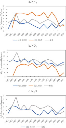
The total emissions of NH₃ from biomass burning ranged from 3.74 Tg year⁻¹ to 5.87 Tg year⁻¹, with an average total of 4.53 ± 0.51 Tg NH₃ year⁻¹ emitted over the period. These emissions are approximately 9% of total global ammonia emissions (Schlesinger and Bernhardt 2013). The total annual emissions of NO_x from biomass burning ranged from 12.21 Tg year⁻¹ to 18.95 Tg year⁻¹, with an average total of 14.65 ± 1.60 Tg NO_x year⁻¹ emitted over the period. This represents 27% of the total global NO_x emissions (Schlesinger and Bernhardt 2013). The total annual emissions of N₂O from biomass burning ranged from 0.80 Tg year⁻¹ to 1.26 Tg year⁻¹, with an average total of 0.97 ± 0.11 Tg N₂O year⁻¹ emitted over the period. Emissions from N₂O from biomass burning account for approximately 6% of all global N₂O emissions (Schlesinger and Bernhardt 2013). On a global scale, these emissions were comparable with the literature (Table 5).

Table 5. Comparison against average annual total yearly emissions from biomass burning in the literature

	NH3 Tg year^−1	NOx Tg year^−1	N2O Tg year^−1
This study	4.5 ± 0.5	14.7 ± 1.6	1.0 ± 0.1
Wiedinmyer et al. (2011) (FINNv1)	4.5 ± 0.7	12.5 ± 1.05	-
FINNv1.4	5.2 ± 0.9	11.3 ± 2.1	-
Kaiser et al. (2012) (GFASv1)	7.7	9.5	0.9
Kaiser et al. (2012) (GFEDv3.1)	-	9.4	0.8
GFEDv4	4.1 ± 0.5	13.1 ± 3.4	0.9 ± 0.1
Lamarque et al. (2010)	6.2 ± 2.3	9.8 ± 1.3	-
Andreae and Merlet (2001)	10.3	20.7	1.3
Andreae (2019)	10	19	1.36
Schlesinger and Bernhardt (2013)	7.7	9.6	0.9

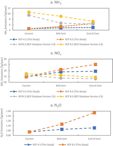
To examine the potential impact of climate change on emissions of NH₃, NO_x, and N₂O from biomass burning, the regressions were run using future burn area projections based on the RCP 4.5 and RCP 8.5 climate scenarios for two time periods: mid-century (2050–2055) and end of century (2090–2095). The results of these model runs are shown in Figure 2. By mid-century, the average yearly total NH₃ emissions are projected to be ~ 4.83 ± ~6.26 Tg year⁻¹ rising to ~4.97 ± ~0.24 Tg year⁻¹ by the end of the century under the RCP 4.5 climate scenario. Under the RCP 8.5 climate scenario, average NH₃ emissions from biomass burning are projected to increase to ~5.32 ± ~0.33 Tg year⁻¹ by mid-century and increase to ~6.39 ± ~.77 Tg year⁻¹ by the end of the century. NO_x emissions from biomass burning are projected to increase to ~18.9 ± ~2.54 Tg year⁻¹ by mid-century and by the end of the century increase to ~19.5 ± ~0.95 Tg year⁻¹ under the RCP 4.5 climate scenario. The average annual NO_x emissions from biomass burning are projected to increase to ~20.9 ± ~1.33 Tg year⁻¹ by mid-century and increase to ~25.3 ± ~3.05 Tg year⁻¹ by the end of the century under the RCP 8.5 climate scenario. Under the RCP 4.5 climate scenario, average annual emissions of N₂O are projected to increase mid-century to ~1.02 ± ~0.14 Tg year⁻¹ and then to ~1.05 ± ~ 0.05 Tg year⁻¹ by the end of the century. The RCP 8.5 climate scenario projects a higher increase in emissions, with average N₂O emissions from biomass burning reaching ~1.13 ± ~0.07 Tg year⁻¹ by mid-century and by the end of the century increasing to ~1.37 ± ~0.16 Tg year⁻¹. Under both the RCP 4.5 and RCP 8.5 climate scenario, these regression models project emissions of NH₃, NO_x and N₂O to increase through the period to the end of the century, all other factors being equal. This could potentially have significant impacts on the global nitrogen cycle. Interestingly, opposite results were projected for emissions of NO_x and NH₃ from biomass burning (savannah burning and forest fires) under both scenarios from the RCP Database version 2.0 (Clarke et al. 2007; Hurtt et al. 2011; Riahi et al., 2007; Smith and Wigley 2006; Van Der Werf et al. 2006; Wise et al. 2009). However, while the trends were the opposite, emissions of NH₃ under both climate scenarios were higher than those predicted in this study (Figure 2(a)). In contrast to this, emissions of NO_x start out similar to current observations, while future projections are lower than what is predicted in this work (Figure 2(b)). Lamarque et al. (2013) shows NO_x emissions from biomass burning decreasing through the end of the century under both RCP scenarios; however, emissions of NH₃ are projected to increase. These differences can be attributed to differences in the model input, for example, differences in projected fire estimates, vegetation composition and distribution, global land use, and meteorological conditions. It is important to recall that there are several assumptions associated with these emission estimates. For an example, these models were created under the assumption that the emission factors will still hold true under the changing climate and that the relationship between emissions and burn area will remain constant.

Figure 2. Comparing current average yearly estimated emissions from biomass burning for NH₃ (a), NO_x (b) and N₂O (c) with projected future yearly emissions based off two climate change scenarios: RCP 4.5 and RCP 8.5. Emissions of NH₃ and NO_x from biomass burning are also compared with future emissions from the RCP Database Version 2.0. The “Current” time frame refers to the study period (2001–2015), “Mid-Century” refers to 2050–2055, and “End of Century” refers to 2090–2095. The RCP Database, which is represented by the yellow and gray lines, can be accessed at https://tntcat.iiasa.ac.at/RcpDb/dsd?Action=htmlpage&page=welcome

Conclusion

NH₃, NO_x, and N₂O emissions from biomass burning were estimated at a global scale for 2001–2015 using a suite of satellite data. On average, 4.53 ± 0.51 Tg NH₃ year⁻¹, 14.65 ± 1.60 Tg NO_x year⁻¹, and 0.97 ± 0.11 Tg N₂O year⁻¹ were emitted from biomass burning over the period, which are comparable with other major emissions inventories. In order to determine the impact of climate change on emissions of NH₃, NO_x, and N₂O, statistical observation models were created for each species to predict future average emissions as a function of future average burn area. The regression models performed fairly well when run for the last portion of the study period (2011–2015) and compared against the emissions calculated in this study. These regressions were then run for two future time periods: 2050–2055 (“mid-century”) and 2090–2095 (“end of century”) and found that emissions of NH₃, NO_x, and N₂O are projected to increase under both climate scenarios by the end of the century, all other factors being equal. These changes are likely due to projected changes to meteorology and biomass burning activity (i.e., increase in global temperature and a decrease in precipitation which results in an increase in burn area) as well as likely due to changes in land use.

Acknowledgment

The authors thank the China Section of the Air & Waste Management Association for the generous scholarship they received to cover the cost of page charges, and make the publication of this article possible.

The authors would like to acknowledge and thank Dr. Maria Val Martin for generously providing the data for future burn area as well as for the guidance provided on the dataset. We would like to acknowledge the NCAR GIS Program for providing the NCAR Climate System Model (CCSM) RCP climate scenario projections, which are freely available from https://gisclimatechange.ucar.edu/. The authors acknowledge the University of Maryland, Department of Geography, Global Land Cover Facility and NASA for generously providing the MODIS Cover data, which is freely available at http://glcf.umd.edu/data/lc/. The authors acknowledge NASA for providing the Making Earth Science Data Records for Use in Research Environments (MEaSUREs) vegetation data from the LP DAAC webpage; https://lpdaac.usgs.gov/dataset_discovery/measures/measures_products_table/vcf5kyr_v001. The authors also acknowledge the University of Maryland for generously providing the MODIS burn area data, which are freely available from http://modis-fire.umd.edu/ba.html. The authors also acknowledge and thank NASA for providing the MERRA-2 data on their website(https://disc.gsfc.nasa.gov/datasets/M2TMNXSLV_V5.12.4/summary?keywords=%22MERRA-2%22%20M2TMNXSLV) as well as the Global Precipitation Climatology Centre (GPCC, http://gpcc.dwd.de/) at Deutscher Wetterdienst for providing a global, gridded monthly total precipitation dataset freely available at ftp://ftp.dwd.de/pub/data/gpcc/html/fulldata-monthly_v2018_doi_download.html. The authors acknowledge Dr. Christine Wiedinmyer and NCAR for the providing the FINN data free of charge from https://www2.acom.ucar.edu/modeling/finn-fire-inventory-ncar and Dr. Guido van der Werf et al. for providing the GFED data free of charge from http://www.globalfiredata.org/. Finally, the authors would also like to acknowledge and thank Dr. Venkatesh Rao for the guidance provided on this work.

Disclosure statement

No potential conflict of interest was reported by the authors.

Additional information

Notes on contributors

Casey D. Bray

Casey D. Bray completed her Ph.D. at North Carolina State University under the advisement of Dr. Viney P. Aneja studying the impact of biomass burning on nitrogen emissions. She is currently employed as a physical scientist with the US EPA.

William H. Battye

William H. Battye has worked for 40 years as a consultant in the environmental industry, with a specialty in air pollution and air pollution control. His work has included measurement and modeling of air pollution, and technical and economic analysis of pollution controls. For 25 years, he served as managing partner of EC/R Incorporated, a firm which provided contract consulting services to the U.S. Environmental Protection Agency and other governmental agencies. He is a registered Professional Engineer and holds B.S. and M.S. Degrees in Chemical Engineering from the Massachusetts Institute of Technology, and a Ph.D. in Marine, Earth and Atmospheric Sciences from North Carolina State University.

Viney P. Aneja

Viney P. Aneja is a Professor in the Department of Marine, Earth, and Atmospheric Sciences, North Carolina State University. Before joining the faculty of the Department of Marine, Earth, and Atmospheric Sciences at N. C. State in 1987, he conducted and supervised research at Corporate Research and Development, General Electric Company, New York; and Northrop Service, in Research Triangle Park, NC, in the areas of environmental science and engineering and separations technology. In 2001 he was also appointed Professor of Environmental Technology, Department of Forestry and Environmental Resources. In addition, he has been a visiting professor at the University of Uppsala, Sweden in 1979; at the Arrhenius Laboratory in Stockholm, Sweden in 1985 and 2015; and the Indian Institute of Technology, Kanpur, India, 2015. He holds a B. Tech. in chemical engineering from the Indian Institute of Technology, a M.S. in chemical engineering from North Carolina State University and a Ph.D. in chemical engineering from North Carolina State University.

William H. Schlesinger

William H. Schlesinger is a biogeochemist and the retired president of the Cary Institute of Ecosystem Studies, an independent not-for-profit environmental research organization in Millbrook, New York.

References

- Akagi, S. K., R. J. Yokelson, C. Wiedinmyer, M. J. Alvarado, J. S. Reid, T. Karl, J. D. Crounse, and P. O. Wennberg. 2011. Emission factors for open and domestic biomass burning for use in atmospheric models. Atmos. Chem. Phys. 11 (9):4039– 72.
- Andreae, M. O. 2019. Emission of trace gases and aerosols from biomass burning–an updated assessment. Atmos. Chem. Phys. 19 (13):8523–46. doi:10.5194/acp-19-8523-2019.
- Andreae, M. O., and P. Merlet. 2001. Emission of trace gases and aerosols from biomass burning. Global Biogeochem. Cycles 15 (4):955–66. doi:10.1029/2000GB001382.
- Baek, B. H., and V. P. Aneja. 2004. Measurement and analysis of the relationship between ammonia, acid gases, and fine particles in eastern North Carolina. J. Air Waste Manage. Assoc. 54 (5):623–33. doi:10.1080/10473289.2004.10470933.
- Baek, B. H., V. P. Aneja, and Q. Tong. 2004. Chemical coupling between ammonia, acid gases, and fine particles. Environ. Pollut. 129 (1):89–98. doi:10.1016/j.envpol.2003.09.022.
- Battye, W., V. P. Aneja, and W. H. Schlesinger. 2017. Is nitrogen the next carbon? Earth’s Future 5 (9):894–904. doi:10.1002/2017EF000592.
- Behera, S. N., and M. Sharma. 2010. Investigating the potential role of ammonia in ion chemistry of fine particulate matter formation for an urban environment. Sci. Total Environ. 408 (17):3569–75. doi:10.1016/j.scitotenv.2010.04.017.
- Bobbink, R., K. Hicks, J. Galloway, T. Spranger, R. Alkemade, M. Ashmore, M. Bustamante, S. Cinderby, E. Davidson, F. Dentener, et al. 2010. Global assessment of nitrogen deposition effects on terrestrial plant diversity: A synthesis. Ecol. Appl. 20(1):30–59. doi:10.1890/08-1140.1.
- Bobbink, R., M. Hornung, and J. G. M. Roelofs. 1998. The effects of air‐borne nitrogen pollutants on species diversity in natural and semi‐natural European vegetation. J. Ecol. 86 (5):717–38.
- Bosilovich, M. G., F. R. Robertson, and J. Chen. 2011. Global energy and water budgets in MERRA. J. Clim. 24 (22):5721–39. doi:10.1175/2011JCLI4175.1.
- Bouwman, A. F. 1996. Direct emission of nitrous oxide from agricultural soils. Nutr. Cycling Agroecosyst. 46 (1):53–70. doi:10.1007/BF00210224.
- Bray, C. D. 2019. Reactive nitrogen emissions from biomass burning and the impact of climate change.
- Channan, S., K. Collins, and W. R. Emanuel. 2014. Global mosaics of the standard MODIS land cover type data, College Park, Maryland, USA: University of Maryland and the Pacific Northwest National Laboratory. 30.
- Chen, X., D. Day, B. Schichtel, W. Malm, A. K. Matzoll, J. Mojica, C. E. McDade, E. D. Hardison, D. L. Hardison, S. Walters, et al. 2014. Seasonal ambient ammonia and ammonium concentrations in a pilot IMPROVE NHx monitoring network in the western United States. Atmos. Environ. 91:118–26. doi:10.1016/j.atmosenv.2014.03.058.
- Clark, C. M., and D. Tilman. 2008. Loss of plant species after chronic low-level nitrogen deposition to prairie grasslands. Nature 451 (7179):712–15. doi:10.1038/nature06503.
- Clarke, L., J. Edmonds, H. Jacoby, H. Pitcher, J. Reilly, and R. Richels. 2007. Scenarios of greenhouse gas emissions and atmospheric concentrations.
- Crutzen, P. J., L. E. Heidt, J. P. Krasnec, W. H. Pollock, and W. Seiler. 2016. Biomass burning as a source of atmospheric gases CO, H2, N2O, NO, CH3Cl and COS. In A pioneer on atmospheric chemistry and climate change in the anthropocene, ed. P. J. Crutzen, 117–124. Cham: Springer.
- Crutzen, P. J., L. E. Heidt, J. P. Krasnec, W. H. Pollock, and W. Seiler. 1979. Biomass burning as a source of atmospheric gases CO, H2, N2O, NO, CH3Cl and COS. Nature 282 (5736):253–56. doi:10.1038/282253a0.
- Davidson, E. A., M. B. David, J. N. Galloway, C. L. Goodale, R. Haeuber, J. A. Harrison, R. W. Howarth, D. B. Jaynes, R. R. Lowrance, B. T. Nolan, et al. 2011. Excess nitrogen in the US environment: Trends, risks, and solutions. Issues Ecol. 15: 1–16.
- Day, D. E., X. Chen, K. A. Gebhart, C. M. Carrico, F. M. Schwandner, K. B. Benedict, B. A. Schichtel, and J. L. Collett Jr. 2012. Spatial and temporal variability of ammonia and other inorganic aerosol species. Atmos. Environ. 61:490–98. doi:10.1016/j.atmosenv.2012.06.045.
- Erisman, J. W., J. N. Galloway, S. Seitzinger, A. Bleeker, N. B. Dise, A. M. R. Petrescu, A. M. Leach, and W. de Vries. 2013. Consequences of human modification of the global nitrogen cycle. Philos. Trans. R. Soc. 368 (1621):20130116. doi:10.1098/rstb.2013.0116.
- Fan, J., R. Zhang, G. Li, J. Nielsen‐Gammon, and Z. Li. 2005. Simulations of fine particulate matter (PM2. 5) in Houston, Texas. J. Geophys. Res. A: Atmos 110 (16). doi:10.1029/2005JD005805.
- Ferreira-Leite, F., A. Bento-Gonçalves, A. Vieira, and L. da Vinha. 2015. Mega-fires around the world: A literature review. In Wildland fires: A worldwide reality, eds. A. J. Bento Gonçalves, A. A. Batista Vieira, 15–33.
- Friedl, M. A., D. Sulla-Menashe, B. Tan, A. Schneider, N. Ramankutty, A. Sibley, and X. Huang. 2010. MODIS collection 5 global land cover: Algorithm refinements and characterization of new datasets. Remote Sens. Environ. 114 (1):168–82. doi:10.1016/j.rse.2009.08.016.
- Galloway, J. N., F. J. Dentener, D. G. Capone, E. W. Boyer, R. W. Howarth, S. P. Seitzinger, G. P. Asner, C. C. Cleveland, P. A. Green, E. A. Holland, et al. 2004. Nitrogen cycles: Past, present, and future. Biogeochemistry 70 (2):153–226.
- Gelaro, R., W. McCarty, M. J. Suárez, R. Todling, A. Molod, L. Takacs, C. A. Randles, A. Darmenov, M. G. Bosilovich, R. Reichle. 2017. The modern-era retrospective analysis for research and applications, version 2 (MERRA-2). J. Clim. 30 (14):5419–54.
- Giglio, L., C. O. Justice, L. Boschetti, and D. P. Roy. 2015. MCD64A1 MODIS/Terra+Aqua Burned Area Monthly L3 Global 500m SIN Grid V006 (dataset). NASA EOSDIS Land Processes DAAC. Accessed January 12, 2019. https://doi.org/10.5067/MODIS/MCD64A1.006.
- Gilbert, R. O. 1987. Statistical methods for environmental pollution monitoring. New York: John Wiley & Sons.
- Gruber, N., and J. N. Galloway. 2008. An earth-system perspective of the global nitrogen cycle. Nature 451 (7176):293–96. doi:10.1038/nature06592.
- Hansen, M., and X. P. Song. 2018. Vegetation continuous fields (VCF) yearly global 0.05 deg. NASA EOSDIS land processes DAAC.
- Hausfather, Z., and G. P. Peters. 2020. Emissions–the ‘business as usual’story is misleading. 618–20.
- Heald, C. L., J. L. Collett Jr, T. Lee, K. B. Benedict, F. M. Schwandner, Y. Li, L. Clarisse, D. R. Hurtmans, M. Van Damme, C. Clerbaux. 2012. Atmospheric ammonia and particulate inorganic nitrogen over the United States.
- Hoelzemann, J. J. 2004. Global wildland fire emission model (GWEM): Evaluating the use of global area burnt satellite data. J. Geophys. Res. A: Atmos. 109 (D14). doi:10.1029/2003JD003666.
- Hoffmann, A. A., P. D. Rymer, M. Byrne, K. X. Ruthrof, J. Whinam, M. McGeoch, D. M. Bergstrom, G. R. Guerin, B. Sparrow, L. Joseph, et al. 2019. Impacts of recent climate change on terrestrial flora and fauna: Some emerging Australian examples. Austral. Ecol. 44(1):3–27. doi:10.1111/aec.12674.
- Holtgrieve, G. W., D. E. Schindler, W. O. Hobbs, P. R. Leavitt, E. J. Ward, L. Bunting, G. Chen, B. P. Finney, I. Gregory-Eaves, S. Holmgren, et al. 2011. A coherent signature of anthropogenic nitrogen deposition to remote watersheds of the northern hemisphere. Science. 334(6062):1545–48. doi:10.1126/science.1212267.
- Houghton, R. A., J. L. Hackler, and R. M. Cushman. 2001. Carbon flux to the atmosphere from land-use changes: 1850 to 1990. Oak Ridge: Carbon Dioxide Information Center, Environmental Sciences Division, Oak Ridge National Laboratory.
- Hurtt, G. C., L. P. Chini, S. Frolking, R. A. Betts, J. Feddema, G. Fischer, J. P. Fisk, K. Hibbard, R. A. Houghton, A. Janetos, et al. 2011. Harmonization of land-use scenarios for the period 1500–2100: 600 years of global gridded annual land-use transitions, wood harvest, and resulting secondary lands. Clim. Change. 109(1–2):117. doi:10.1007/s10584-011-0153-2.
- Ito, A. 2004. Global estimates of biomass burning emissions based on satellite imagery for the year 2000. J. Geophys. Res. A: Atmos. 109 (D14). doi:10.1029/2003JD004423.
- Janssens, I. A., W. Dieleman, S. Luyssaert, J.-A. Subke, M. Reichstein, R. Ceulemans, P. Ciais, A. J. Dolman, J. Grace, G. Matteucci, et al. 2010. Reduction of forest soil respiration in response to nitrogen deposition. Nat. Geosci. 3(5):315–22. doi:10.1038/ngeo844.
- Kaiser, J. W., A. Heil, M. O. Andreae, A. Benedetti, N. Chubarova, L. Jones, -J.-J. Morcrette, M. Razinger, M. G. Schultz, M. Suttie, et al. 2012. Biomass burning emissions estimated with a global fire assimilation system based on observed fire radiative power. Biogeosciences. 9(1):527. doi:10.5194/bg-9-527-2012.
- Kendall, M. G. 1975. Rank correlation methods. London: Charles Griffin & Co.
- Kleist, D. T., D. F. Parrish, J. C. Derber, R. Treadon, W.-S. Wu, and S. Lord. 2009. Introduction of the GSI into the NCEP global data assimilation system. Weather and Forecasting 24 (6):1691–705. doi:10.1175/2009WAF2222201.1.
- Lamarque, J.-F., T. C. Bond, V. Eyring, C. Granier, A. Heil, Z. Klimont, D. Lee, C. Liousse, A. Mieville, B. Owen, et al. 2010. Historical (1850–2000) gridded anthropogenic and biomass burning emissions of reactive gases and aerosols: Methodology and application.
- Lamarque, J.-F., F. Dentener, J. McConnell, C-U. Ro, M. Shaw, R. Vet, D. Bergmann, et al. 2013. Multi-model mean nitrogen and sulfur deposition from the Atmospheric Chemistry and Climate Model Intercomparison Project (ACCMIP): evaluation of historical and projected future changes. Atmos. Chem Phys. 13 (16):7997–8018
- Langford, A. O., F. C. Fehsenfeld, J. Zachariassen, and D. S. Schimel. 1992. Gaseous ammonia fluxes and background concentrations in terrestrial ecosystems of the United States. Global Biogeochem. Cycles 6 (4):459–83. doi:10.1029/92GB02123.
- Lelieveld, J., J. S. Evans, M. Fnais, D. Giannadaki, and A. Pozzer. 2015. The contribution of outdoor air pollution sources to premature mortality on a global scale. Nature 525 (7569):367–71. doi:10.1038/nature15371.
- Li, F., S. Levis, and D. S. Ward. 2013. Quantifying the role of fire in the Earth system–Part 1: Improved global fire modeling in the Community Earth System Model (CESM1). Biogeosciences. 10 (4): 2293–2314.
- Li, F., B. Bond-Lamberty, and S. Levis. 2014. Quantifying the role of fire in the earth system – Part 2: Impact on the net carbon balance of global terrestrial ecosystems for the 20th century. Biogeosciences 11 (5):1345–60. doi:10.5194/bg-11-1345-2014.
- Li, F., D. M. Lawrence, and B. Bond-Lamberty. 2017. Impact of fire on global land surface air temperature and energy budget for the 20th century due to changes within ecosystems. Environ. Res. Lett. 12 (4):044014. doi:10.1088/1748-9326/aa6685.
- Li, F., X. D. Zeng, and S. Levis. 2012. A process-based fire parameterization of intermediate complexity in a dynamic global vegetation model. Biogeosciences 9 (7):2761–80. doi:10.5194/bg-9-2761-2012.
- Liu, Y., J. Stanturf, and S. Goodrick. 2010. Trends in global wildfire potential in a changing climate. For. Ecol. Manage. 259 (4):685–97. doi:10.1016/j.foreco.2009.09.002.
- Lobert, J. M., D. H. Scharffe, W. M. Hao, and P. J. Crutzen. 1990. Importance of biomass burning in the atmospheric budgets of nitrogen-containing gases. Nature 346 (6284):552–54. doi:10.1038/346552a0.
- Macedo, I. C., J. E. A. Seabra, and J. Ear Silva. 2008. Green house gases emissions in the production and use of ethanol from sugarcane in Brazil: the 2005/2006 averages and a prediction for 2020. Biomass Bioenergy. 32 (7): 582–95.
- Mann, H. B. 1945. Nonparametric tests against trend. Econometrica 13 (3):245–59. doi:10.2307/1907187.
- Molod, A., L. Takacs, M. Suarez, and J. Bacmeister. 2015. Development of the GEOS-5 atmospheric general circulation model: Evolution from MERRA to MERRA2. Geosci. Model Dev. 8 (5):1339–56. doi:10.5194/gmd-8-1339-2015.
- Pachauri, R. K., M. R. Allen, V. R. Barros, J. Broome, W. Cramer, R. Christ, J. A. Church, L.. Clarke, Q. Dahe, P. Dasgupta, et al. 2014. Climate change 2014: synthesis report. Contribution of working groups I, II and III to the fifth assessment report of the intergovernmental panel on climate change. IPCC.
- Pierce, J. R., M. Val Martin, and C. L. Heald. 2017. Estimating the effects of changing climate on fires and consequences for US air quality, using a set of global and regional climate models–Final report to the joint fire science program. Fort Collins, CO: Joint Fire Science Program.
- Pope, C. A., III, and D. W. Dockery. 2006. Health effects of fine particulate air pollution: Lines that connect. JAWMA 56 (6):709–42.
- Pope, C. A., III, M. Ezzati, and D. W. Dockery. 2009. Fine-particulate air pollution and life expectancy in the United States. N. Engl. J. Med. 360 (4):376–86. doi:10.1056/NEJMsa0805646.
- Pyne, S. J., P. L. Andrews, and R. D. Laven. 1996. Fire ecology. Introduction to wildland fire, 171–212. second ed. New York: John Wiley & Sons Inc.
- Randerson, J. T., G. R. Van der Werf, L. Giglio, G. J. Collatz, and P. S. Kasibhatla. 2007. Global fire emissions database, version 2 (GFEDv2. 1). Data set. Oak Ridge, Tennessee, USA: Oak Ridge National Laboratory Distributed Active Archive Center. http://daac.ornl.gov/
- Riahi, K., A. Grübler, and N. Nakicenovic. 2007. Scenarios of long-term socio-economic and environmental development under climate stabilization. Technol. Forecast Soc. Change 74 (7):887–935. doi:10.1016/j.techfore.2006.05.026.
- Riahi, K., S. Rao, V. Krey, C. Cho, V. Chirkov, G. Fischer, G. Kindermann, N. Nakicenovic, and P. Rafaj. 2011. RCP 8.5—A scenario of comparatively high greenhouse gas emissions. Clim. Change 109 (1–2):33. doi:10.1007/s10584-011-0149-y.
- Rienecker, M. M., M. J. Suarez, R. Gelaro, R. Todling, J. Bacmeister, E. Liu, M. G. Bosilovich, S. D. Schubert, L. Takacs, G.-K. Kim, et al. 2011. MERRA: NASA’s modern-era retrospective analysis for research and applications. J. Clim. 24(14):3624–48. doi:10.1175/JCLI-D-11-00015.1.
- Robarge, W. P., J. T. Walker, R. B. McCulloch, and G. Murray. 2002. Atmospheric concentrations of ammonia and ammonium at an agricultural site in the southeast United States. Atmos. Environ. 36 (10):1661–74. doi:10.1016/S1352-2310(02)00171-1.
- Roberts, J. M., C. E. Stockwell, R. J. Yokelson, J. de Gouw, Y. Liu, V. Selimovic, A. R. Koss, K. Sekimoto, M. M. Coggon, B. Yuan, et al. 2020. The nitrogen budget of laboratory-simulated western US wildfires during the FIREX 2016 fire lab study. Atmos. Chem. Phys. 20(14):8807–26. doi:10.5194/acp-20-8807-2020.
- Robertson, F. R., M. G. Bosilovich, J. Chen, and T. L. Miller. 2011. The effect of satellite observing system changes on MERRA water and energy fluxes. J. Clim. 24 (20):5197–217. doi:10.1175/2011JCLI4227.1.
- Roy, D. P. 1999. Multi-temporal active-fire based burn scar detection algorithm. Int J Remote Sens. 20 (5):1031–38.
- Roy, D. P., and L. Boschetti. 2009. Southern Africa validation of the MODIS, L3JRC, and GlobCarbon burned-area products. IEEE Trans. Geosci. Remote Sens. 47 (4):1032–44.
- Roy, D. P., L. Boschetti, C. O. Justice, and J. Ju. 2008. The collection 5 MODIS burned area product—Global evaluation by comparison with the MODIS active fire product. Remote Sens. Environ. 112 (9):3690–707.
- Roy, D. P., P. E. Lewis, and C. O. Justice. 2002. Burned area mapping using multi-temporal moderate spatial resolution data—A bi-directional reflectance model-based expectation approach. Remote Sens. Environ. 83 (1–2):263–86.
- Roy, D. P., Y. Jin, P. E. Lewis, and C. O. Justice. 2005. Prototyping a global algorithm for systematic fire-affected area mapping using MODIS time series data. Remote Sens. Environ. 97 (2):137–62.
- Rudolf, B., A. Becker, U. Schneider, A. Meyer-Christoffer, and M. Ziese. 2011. New GPCC full data reanalysis version 5 provides high-quality gridded monthly precipitation data. Gewex News 21 (2):4–5.
- Schlesinger, W. H., and E. S. Bernhardt. 2013. Biogeochemistry: An analysis of global change, 15–48. Cambridge, MA: Academic Press.
- Schneider, U., T. Fuchs, A. Meyer-Christoffer, and B. Rudolf. 2008. Global precipitation analysis products of the GPCC. Global Precipitation Climatol. 112.
- Seiler, W., and P. J. Crutzen. 1980. Estimates of gross and net fluxes of carbon between the biosphere and the atmosphere from biomass burning. Clim. Change 2:207–47.
- Smith, S. J., and T. M. L. Wigley. 2006. Multi-gas forcing stabilization with Minicam. Energy J. Spec. Issue 3: 373–391.
- Suarez, M. J., M. Rienecker, R. Todling, J. Bacmeister, L. Takacs, H. Liu, W. Gu, M. Sienkiewicz, R. Koster, and R. Gelaro. 2008. The GEOS-5 data assimilation system-documentation of versions 5.0. 1, 5.1. 0, and 5.2.
- Syphard, A. D., and J. E. Keeley. 2015. Location, timing and extent of wildfire vary by cause of ignition. Int. J. Wildland Fire 24(1): 37–47.
- Syphard, A. D., J. E. Keeley, A. H. Pfaff, and K. Ferschweiler. 2017. Human presence diminishes the importance of climate in driving fire activity across the United States. Proc. Natl. Acad. Sci. 114 (52):13750–55.
- Thomson, A. M., K. V. Calvin, S. J. Smith, G. Page Kyle, A. Volke, P. Patel, S. Delgado-Arias, B. Bond-Lamberty, M. A. Wise, L. E. Clarke, et al. 2011. RCP4. 5: A pathway for stabilization of radiative forcing by 2100. Clim. Change 109 (1–2):77.
- Urbanski, S. 2014. Wildland fire emissions, carbon, and climate: Emission factors. For. Ecol. Manage. 317:51–60.
- Val Martin, M., J. R. Pierce, and C. L. Heald. 2018. Global fire emissions, fire area burned and air quality data projected using a global earth system model (RCP45/SSP1 and RCP8. 5/SSP3).
- Van Der Werf, G. R., J. T. Randerson, L. Giglio, G. J. Collatz, P. S. Kasibhatla, and A. F. Arellano Jr. 2006. Interannual variability of global biomass burning emissions from 1997 to 2004.
- Van Der Werf, G. R., J. T. Randerson, L. Giglio, T. T. Van Leeuwen, Y. Chen, B. M. Rogers, M. Mu, M. J. Van Marle, D. C. Morton, G. J. Collatz, et al. 2017. Global fire emissions estimates during 1997–2016. Earth Syst. Sci. Data 9 (2):697–720.
- Van Leeuwen, T. T., and G. R. Van Der Werf. 2011. Spatial and temporal variability in the ratio of trace gases emitted from biomass burning. Atmos. Chem. Phys. 11 (8):3611.
- Van Leeuwen, T. T., W. Peters, M. C. Krol, and G. R. Van Der Werf. 2013. Dynamic biomass burning emission factors and their impact on atmospheric CO mixing ratios. J. Geophys. Res. A: Atmos. 118 (12):6797–815.
- Van Vuuren, D. P., J. Edmonds, M. Kainuma, K. Riahi, A. Thomson, K. Hibbard, G. C. Hurtt, et al. 2011a. The representative concentration pathways: An overview. Clim. Change 109 (1–2):5.
- van Vuuren, D. P., L. F. Bouwman, S. J. Smith, and F. Dentener. 2011b. Global projections for anthropogenic reactive nitrogen emissions to the atmosphere: An assessment of scenarios in the scientific literature. Curr. Opin. Environ Sustainability 3 (5):359–69.
- Wang, X., W. Wang, L. Yang, X. Gao, W. Nie, Y. Yu, P. Xu, Y. Zhou, and Z. Wang. 2012. The secondary formation of inorganic aerosols in the droplet mode through heterogeneous aqueous reactions under haze conditions. Atmos. Environ. 63:68–76.
- Wiedinmyer, C., B. Quayle, C. Geron, A. Belote, D. McKenzie, X. Zhang, S. O’Neill, and K. K. Wynne. 2006. Estimating emissions from fires in North America for air quality modeling. Atmos. Environ. 40 (19):3419–32.
- Wiedinmyer, C., S. K. Akagi, R. J. Yokelson, L. K. Emmons, J. A. Al-Saadi, J. J. Orlando, and A. J. Soja. 2011. The fire inventory from NCAR (FINN): A high resolution global model to estimate the emissions from open burning. Geosci. Model Dev. 4 (3):625.
- Willmott, C. J., C. M. Rowe, and W. D. Philpot. 1985. Small-scale climate maps: A sensitivity analysis of some common assumptions associated with grid-point interpolation and contouring. Am. Cartographer 12 (1):5–16.
- Wise, M., K. Calvin, A. Thomson, L. Clarke, B. Bond-Lamberty, R. Sands, S. J. Smith, A. Janetos, and J. Edmonds. 2009. Implications of limiting CO2 concentrations for land use and energy. Science 324 (5931):1183–86.
- Wu, W.-S., R. James Purser, and D. F. Parrish. 2002. Three-dimensional variational analysis with spatially inhomogeneous covariances. Mon. Weather Rev. 130 (12):2905–16.