Novel cross-flow electrostatic precipitator: Numerical and experimental study

ABSTRACT

Electrostatic precipitators (ESP) are used extensively for removing particulates from a gas flow by charging the particles and then removing them in the presence of an electric field. Traditional ESP designs use the walls of the flow channel as the grounded collection surface. The objective of this present study is to evaluate a novel ESP configuration, recently patented by Ohio University’s Electrostatic Laboratory, in which an array of vertical surfaces of cylindrical geometry are placed in a crossflow configuration and used as grounded collection surfaces. A numerical approach was adopted by developing and implementing User-Defined Functions (UDFs) in ANSYS Fluent computational fluid dynamics (CFD) software to build a two-dimensional cross-flow ESP model, for the first time, for the gas flow and particulate capture. The two-dimensional numerical models proved useful in shedding light on the basics of the collection process in the novel cross-flow ESP. In the studied configuration, the collection of the particles on the collector surface was limited to the anterior and posterior surfaces of the first and second collection rows, respectively. The collection at the posterior surface of the second row presented interesting behavior, with the particles becoming entrained in the wake of the collectors and the electric field from the discharge electrode located downstream that was opposite to the fluid flow direction. The output of the simulation underestimated the experimental data. The lower efficiency prediction of the model could have been due to the vibration of the collection electrodes, collection by the mist formed in the wet system, and particle agglomeration in the experiments. The results of this study provide critical information in improving the particulate efficiency of novel cross-flow ESP and other similar cross-flow ESP systems.

Implications: A novel Electrostatic precipitator (ESP) configuration (recently patented) was evaluated. A numerical approach was adopted to build a cross-flow ESP model, for the first time, for the gas flow and particulate capture. The collection of the particles on the collector surface was limited to the anterior and posterior surfaces of the first and second collection rows. Also, the particles were entrained in the wake of the collectors. The output of the simulation underestimated the experimental data. The results of this study provide critical information in improving the particulate efficiency of novel cross-flow ESP and other similar cross-flow systems.

Introduction

Electrostatic precipitators (ESPs) have found common utilization as particulate collection systems by treating waste flue gases from plant processes. This can be attributed to their ability to efficiently capture a wide range of particulate sizes under varied operating conditions (pressures, flow rates, exhaust temperatures, etc.) (Crawford 1976; Flagan and Seinfield 1988). Despite these advantages, conventional dry ESPs find difficulty in capturing particles in the submicron range (0.1 µm < $D_p$< 1 µm) (Chen et al. 2014a).

The sub-optimal collection of particles in this range (<70% in comparison to global efficiencies of 99%) expose human populations to severe health dangers, as the human body’s ability to adequately filter particles under 2 µm is greatly compromised (Nicol 2013). In general, the drop in efficiency of the ESP can be attributed to the resistivity of the particle, as well as the particles’ size which contribute to sub-optimal charging of the particulates (Kanazawa et al. 1993; Laitinen et al. 1996). In addition, the accumulation of particulates on the collection surface can lower corona charge levels and limit charging (Ali et al. 2016; Altman, Buckley, and Ray 2001; Altman et al. 2001).

The two possible approaches in improving collection efficiency involve increasing charging on the particles or improving agglomeration of the particles (Kanazawa et al. 1993). A high capital and operating cost of a powering unit is associated with simply increasing the charge on the particle surface. Further, increasing the electric field strength in the precipitation region does little to change the charge on particles under 1 µm in size. However, agglomeration methods could positively influence collection. Agglomeration is simply the coagulation of smaller particles to yield a single particle of larger mean diameter. Many agglomeration techniques have been proposed such as: condensation-induced agglomeration (wet ESP’s (Chang et al. 2017; Chen et al. 2014b)) and electrical agglomeration (unipolar pre-charging (Hautanen et al. 1995), bi-polar pre-charging (Chang et al. 2015, 2017)). The concept of condensation-induced agglomeration relies on the generation of liquid bridges between particles in order to significantly increase adhesive forces between particles and in turn agglomeration. On the other hand, the electrical agglomeration methods utilize AC or DC electric fields to agitate suspended particles within the gas stream.

Alam and Pasic (2017), proposed a novel ESP configuration (patented), the cross-flow ESP, to address a variety of challenges that modern ESPs experience. Among these are the maximization of collection efficiencies in the sub-micron range and the minimization of the system’s footprint as a result of the size and configuration of the collection surface. This technology was studied experimentally and reported by Ali et al. (2016). The system deviated from the conventional ESP configuration, which utilized collector and discharge plates mounted parallel to the flow. Here, the collectors were vertical columns made of permeable material, which were placed perpendicular to the incoming fluid stream (Figure 1). The accumulation of particulates on the collector surface was prevented by the continual introduction of wash fluid (typically water) down the surface of the collector columns. Two rows of collectors were placed between two sets of discharge electrodes; also, in a cross-flow to the incoming flue stream. The expectation of this construction was to utilize the turbulence generated by the flow across the collection columns in agitating the particles in the flow and in turn improving agglomeration. Experiments undertaken showed global particulate collection efficiencies above 80% with two pairs of collectors used (Ali et al. 2016).

Figure 1. Cross-flow schematic (Ali et al. 2016)

The aim of this paper is to develop, for the first time, a numerical modeling approach that describes the flow behavior across the novel cross-flow ESP under standard operating conditions as well as its particulate collection mechanism. Previous studies have focused on modeling other traditional flow field configurations, such as, wire-pipe, wire-plate, and wire-duct ESP’s. In all cases, these configurations correspond to collecting surfaces parallel to the free-stream flow. The present system differs from this in that the collection surface obstructs the free-stream flow. Thus, this creates a unique flow structure that differs considerably from traditional horizontal flow ESP’s. In addition, the implementation of combined charging models ensured adequate charging of a wide range of particle sizes. This involves accounting for diffusion charging and field charging (Farnoosh, Adamiak, and Castle 2011; Fujishima et al. 2004; Gallimberit 1998). This study also focused its efforts on modeling a unit section of the flow domain to capture a higher resolution of the flow structure around the collection surfaces. This is beneficial since the dimensions of the cross-flow setup are complex allowing for a less computationally expensive simulation approach. This work was completed in parallel to the work of the author’s PhD thesis (Eboreime 2019). The purpose of this new and original work is to develop reliable models that will enable inexpensive optimization of the cross-flow ESP configurations in future.

Numerical method

Three physical phenomena primarily govern the ESP’s operation namely: 1) the gas flow, 2) the ionized electric field, and 3) the particulate motion. All aforementioned phenomena are mutually coupled with varying degrees of strength, with the weaker coupling often ignored for simplicity. Figure 2 shows a schematic representation of the phenomena and the mutual coupling between them.

Figure 2. Mutual coupling of physical phenomena in electrostatic precipitators (ESP’s)

Governing equations

Fluid flow field

The fluid flow within an ESP is governed by the standard conservation equations for continuity and momentum for incompressible fluids (Equation 1). The superscript “c” denotes the variables that account for coupling to other phenomena.

(1a) $\mathrm{\nabla }.\left(\overrightarrow{u}\right)=0$(1a)

(1b) $\rho \overrightarrow{u}.\mathrm{\nabla }\overrightarrow{u}=\mathrm{\nabla }p+\mu {\mathrm{\nabla }}^2\vec{u}+S^c$(1b)

where ρ ($kg/m^3$) represents the fluid density, $\overrightarrow{u}\left(m/s\right)$ represents the fluid velocity, $\mathrm{p}\left(Pa\right)$ represents the pressure, and $\mu \left(Pa.s\right)$ represents the fluid viscosity. The source term $S^c$ represents the imposed body force by the electric field$\left(S^c=q^c\overrightarrow{E}\right)$, $q\left(C/m^3\right)$represents the charge density in the field, while the variable $\overrightarrow{E}\left(V/m\right)$ represents the electric field strength.

Electric field

Ionic discharge from the discharge electrodes results in charged flow due to induced electric field. Ideally, an ionization layer exists at the discharge electrode consisting of both positively and negatively charged ions. Although attempts have been made to model the ionization layer, the most common approach is to model discharge electrodes by assuming single specific ionic flow (Feng, Long, and Adamiak 2016).

The electric field model is governed by the set of relevant Maxwell’s equations; given the fact that there are no imposed magnetic fields in the system. The relevant equations are reduced to Gauss’s law and Ampere’s law (Equation 2).

(2a) $\mathrm{\nabla }.\overrightarrow{E}=\left(\frac{q+q_p^c}{{\epsilon }_o}\right)$(2a)

(2b) $\mathrm{\nabla }\cdot \overrightarrow{J}=0$(2b)

The charge density in the precipitation zone is governed by Gauss’ law which simply states that the electric field is produced as a result of the density of the electric charge. The variable $q\left(C/m^3\right)$represents the contribution to the electric space charge density as a result of moving ions in the stream while the variable $q_p^c\left(C/m^3\right)$ represents the contribution due to the already charged particles in the stream. The dielectric permittivity of the medium (in this case air) is defined by ${\epsilon }_0\left(F/m\right)$ which represents the resistance to charge flux in the medium.

The current density $\left(\overrightarrow{J}\right)$ results from the combination of three distinct phenomena. The independent motion of ions through the medium relative to the airflow (conductive), the bulk transport of the ions through the medium by the airflow (advective), and the diffusive transport of ions across the concentration gradient (diffusive). Equation 3(3) $\overrightarrow{J}=b_i\left(q+q_p^c\right)\overrightarrow{E}+\left(q+q_p^c\right)\overrightarrow{u}-D_i\mathrm{\nabla }\left(q+q_p^c\right)$(3) shows the expression that elaborates on the interaction of these phenomena.

$\begin{array}{c}Current\\ Density\end{array}=\begin{array}{c}Conductive\\ Eqn.\end{array}+\begin{array}{c}Advective\\ Eqn.\end{array}+\begin{array}{c}Diffusive\\ Eqn.\end{array}$

(3) $\overrightarrow{J}=b_i\left(q+q_p^c\right)\overrightarrow{E}+\left(q+q_p^c\right)\overrightarrow{u}-D_i\mathrm{\nabla }\left(q+q_p^c\right)$(3)

Here $b_i\left(m^2/V\cdot s\right)$ denotes the ionic mobility of the ion through the medium as a result of the imposed electric field. The ionic mobility is a measure of the velocity attained by an ion moving through a fluid under unit electric field in${\mathrm{m}}^2/\mathrm{s}\cdot \mathrm{V}$. The variable $D_i\left(m^2/s\right)$ represents the diffusion coefficient of the ions which is the proportionality constant between the flux, due to diffusion, and the concentration gradient of the species.

Particulate transport

Particulate trajectory

The motion of particles through the medium is governed by Newton’s 2^nd law which simply states that the sum of force applied to a body equals the change in momentum per unit time. Assuming a constant mass for each particle this can be reduced to simply the product of particle mass and velocity change as shown in Equation 4(4) $m_p\frac{d\overrightarrow{u}}{dt}=\overrightarrow{F_e}+\overrightarrow{F_d}+\overrightarrow{F_g}$(4) .

(4) $m_p\frac{d\overrightarrow{u}}{dt}=\overrightarrow{F_e}+\overrightarrow{F_d}+\overrightarrow{F_g}$(4)

The summed forces represent the electric force ($\overrightarrow{F_e}$), drag force ($\overrightarrow{F_d}$), and gravitational force ($\overrightarrow{F_g}$) acting at an instance on the particle in the precipitation field. Since the effect of gravity on the particle is very small in comparison to the drag and Coulomb force effects, it can be neglected in the analysis. Also, moment due to rotation of the particle is neglected because their effects on the free-stream behavior are considered negligible due to the particle sizes considered and volume of particles introduced in the present study.

The drag force on the particle is computed using Stokes’ law (Equation 5a(5a) $\overrightarrow{F_d}=\frac{0.5C_D{A}_p{\rho }_{fluid}{V}_{rel}\left(\overrightarrow{V_{rel}}\right)}{C_c}$(5a) ) with the choice of coefficient of drag ($C_D$) values as function of the particles Reynolds Number ($R{e}_p$); as shown in Equation 5b(6) $C_c=1+Kn\left[1.257+0.4exp\left(-\frac{1.1}{Kn}\right)\right]$(6) (Crawford 1976).

(5a) $\overrightarrow{F_d}=\frac{0.5C_D{A}_p{\rho }_{fluid}{V}_{rel}\left(\overrightarrow{V_{rel}}\right)}{C_c}$(5a)

The variable $A_p\left(m^2\right)$represents the projected area of the particle body normal to the flow. The fluid variables are denoted by ${\rho }_{fluid}\left(kg/m^3\right)$ for the fluid density and $\overrightarrow{V_{rel}}\left(m/s\right)$ for the velocity vector of the particle relative to the fluid.

It is also critical to account for the non-continuum effects of the particles transport due to the comparable particle and mean free path sizes. This results in a slip correction factor or Cunningham factor which can generally be neglected for particles exceeding 10 µm. The slip correction factor ($C_c$) is a function of the Knudsen number ($Kn$), as seen in Equation 6(6) $C_c=1+Kn\left[1.257+0.4exp\left(-\frac{1.1}{Kn}\right)\right]$(6) , which itself describes the ratio between the particles diameter ($d_p$) and mean free path ($\lambda$) length scales$\left(Kn=2\lambda /d_p\right)$.

(6) $C_c=1+Kn\left[1.257+0.4exp\left(-\frac{1.1}{Kn}\right)\right]$(6)

The electric force vector ($\overrightarrow{F_e}$) represents the Coulomb force acting on a particle as a result of the imposed electric field in the medium and simply stated as shown in Equation 7(7) $\overrightarrow{F_e}=q_p\overrightarrow{E}$(7) .

(7) $\overrightarrow{F_e}=q_p\overrightarrow{E}$(7)

The variable$q_p$represents the charge magnitude held by the particle at a given instance, and for this reason is a function of the residence time of the particle.

Particulate charging

The particle charge can be estimated by one of the three mechanisms: Field charging, Diffusion charging, and a combined charging method based on both mechanisms (Crawford 1976). The magnitude of charge held is primarily a function of the particle characteristic length, with smaller particles (<0.1 µm) dominated by diffusion charging and larger particles (>1 µm) dominated by field charging. The distribution of particle sizes between the aforementioned bounds experience the charging action of both mechanisms simultaneously.

Field charging becomes prominent as the ion migrating along the electric field flux lines come into the vicinity of the spherical particle thus distorting the flux lines and in turn impinging on the particle (Crawford 1976; Flagan and Seinfield 1988). Although field charging is understood to be a time-dependent mechanism, it is most often assumed that the charge saturation of the particle is attained very rapidly (Crawford 1976; Flagan and Seinfield 1988). Equation 8(8) $q_s=4\pi {ϵ}_0\left(\frac{3\kappa }{\kappa +2}\right)E_{\mathrm{\infty }}{R}_p^2$(8) presents the field charge expression as a function of stream (Permittivity of the medium -${\in }_0$, Dielectric constant -$\kappa$, Electric field magnitude -$E_{\mathrm{\infty }}$) and particle (Particle radius -${\mathfrak{R}}_p$) properties by assuming saturation charge has been reached (Crawford 1976; Flagan and Seinfield 1988).

(8) $q_s=4\pi {ϵ}_0\left(\frac{3\kappa }{\kappa +2}\right)E_{\mathrm{\infty }}{R}_p^2$(8)

On the other hand, diffusion charging (Equation 9(9) $q=\pm \frac{2\pi {ϵ}_0{K}_{B}T{d}_p}{e}\mathrm{I}\mathrm{n}\left(1+\frac{N_i{e}^2{d}_p\overline{c_t}{t}_0}{8{ϵ}_{0}KT}\right)$(9) ; Crawford 1976; Flagan and Seinfield 1988) is a result of random thermal motion of ions colliding with particles and in turn surrendering their charge to the particles (Crawford 1976). Due to the existing charge on both ions and particles, the random thermal motion experienced by the ions is a result of the electrostatic forces existing between both (Crawford 1976). In this case the characteristic length scale of both particle and ion are of the same order of magnitude; therefore, the electric flux is deemed to be primarily dependent on the Knudsen number ($Kn$) of the ion. For this reason, the influence of field charging can be neglected.

(9) $q=\pm \frac{2\pi {ϵ}_0{K}_{B}T{d}_p}{e}\mathrm{I}\mathrm{n}\left(1+\frac{N_i{e}^2{d}_p\overline{c_t}{t}_0}{8{ϵ}_{0}KT}\right)$(9)

The variables $K_B,e,\overline{c_i},T,t_0$ in Equation 9(9) $q=\pm \frac{2\pi {ϵ}_0{K}_{B}T{d}_p}{e}\mathrm{I}\mathrm{n}\left(1+\frac{N_i{e}^2{d}_p\overline{c_t}{t}_0}{8{ϵ}_{0}KT}\right)$(9) denote the Boltzmann constant ($1.38\times 10m^{2}kg/s^2.K$), electron mass, the mean thermal speed of the ions$\left(\sqrt{\frac{8KT}{\pi m_i}}\left(m/s\right)\right)$, absolute temperature ($K$), and the time constant $\left(\frac{4{ϵ}_0}{N_{i}eK}\right)$ in seconds, respectively.

The combination of both charging methods presents the most accurate model, with various studies showing reasonable agreements of experiments with summed charging effects of both mechanisms (Equations 8(8) $q_s=4\pi {ϵ}_0\left(\frac{3\kappa }{\kappa +2}\right)E_{\mathrm{\infty }}{R}_p^2$(8) and 9(10) $E_{onset}=\left({\beta }_1{\rho }_{gas}+{\beta }_2\sqrt{\frac{{\rho }_{gas}}{r_w}}\right)$(10) ; Crawford 1976; Flagan and Seinfield 1988). It should be noted that the assumption of a summed effects does not hold true until field charging has reached saturation condition or closely approached. In estimating saturation time, fair estimates are usually between 10 and 20 times the time constant (Crawford 1976; Flagan and Seinfield 1988).

Computational method

Solution domain model

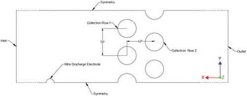
Figure 1 shows the general construction of the cross-flow system. A two-dimensional unit section of the system was utilized as the domain of interest in this study. The cylindrical vertical collector electrodes were modeled with the assumption of a rigid construction and a smooth surface. This was necessary in nullifying the influence of transverse/stream-wise oscillations as well as surface roughness on the flow structures and the particle collection mechanism.

As shown in Figure 3, the domain was rectangular and consisted of two staggered rows of the vertical collectors. Each row was defined by the Transverse-Pitch ($TP$) and Longitudinal-Pitch ($LP$). These variables represented the center-to-center distances between adjacent collectors on the same row and between adjacent rows, respectively. For this study, the diameters of the collectors were uniformly defined at 5 mm, while the$TPand$ $LP$values were defined as 10 mm; this resulted in a pitch-to-diameter ratio of 2. The discharge electrodes modeled in the simulation were reduced to wire electrodes corresponding to the spike tip where corona discharge occurs. This was to reduce model complexity and computational costs within the model. The wire discharge electrodes were 1 mm in diameter and were 70 mm away (center-to-center) from the leading collector electrodes. These dimensions were arbitrarily chosen to develop initial simulations. These numbers were changed later to match with the experimental parameters. In general, closer distances between discharge and collector electrodes would increase the electric field density in the region but may cause sparking issues.

Figure 3. Computational domain for cross-flow electrostatic precipitator (TP, LP = 10 mm; CE diameter = 5 mm; DE diameter = 1 mm)

Mesh

A quadrilateral meshing scheme was employed in the simulations and the ANSYS Fluent meshing environment was used to generate the mesh. A convergence study was conducted, and the following mesh definitions were considered adequate in capturing the behavior. The max mesh size was set to $5\times {10}^{-4}$mm while the minimum mesh size was set to $2.5\times {10}^{-5}$mm; these corresponded to 10% and 0.5%, respectively, of the characteristic length of the vertical collectors. The mesh bordering the collector wall boundaries were specified with an initial height of $2.5\times {10}^{-5}$mm for 20 layers at a growth rate of 5%.

Figure 4 shows the grid generated in the ANSYS meshing environment. As per boundary layer theory, at the smooth solid wall, the fluid velocity is zero, thus the turbulent eddies in the free-stream stop very close to the wall. However, a very thin region separates the free stream behavior from the solid boundary. This region is dominated by viscous effects rather than the inertial effects of the turbulent free-stream. The dimensionless wall-distance $\left(y^{+}\right)$variable provides a measure of the relative importance of viscous and turbulent force as a function of the distance away from the wall. The $y^{+}$ variable is derived from ${\mathrm{u}}_t-$friction velocity, $\mathrm{y}-$is the absolute distance from the wall, and $\nu -$the kinematic viscosity$\left(y^{+}=\frac{{\mathrm{u}}_{t}y}{\nu }\right)\left[20\right]$. In order to adequately resolve flow structures along the boundary, very fine meshes were required to capture behavior of viscous sublayers in this region; ideally $y^{+}<1$ at the cells adjacent to the wall (ANSYS 2015; Versteeg and Malalasekera 2007). In the present study, to ensure that the mesh around the collection electrodes captured the correct flow behavior, the $y^{+}$value at the cells adjacent to collectors were evaluated and averaged in the range of 0.3 to 0.7.

Figure 4. Meshed grid for the cross-flow ESP configuration

Boundary conditions

Two types of boundary conditions were enforced in this study: the hydrodynamic and the electrical boundary conditions. The boundary conditions are detailed in Table 1 below.

Table 1. Hydrodynamic and electrical boundary conditions for the cross-flow model

Boundaries	Hydrodynamic B.C.	Electrical B.C.
Inlet	$u_x=u_{\mathrm{\infty }};u_y=0$
Outlet	Pressure Outlet
Domain Wall Boundaries	Symmetric: $\mathrm{\partial }{u}_y/\mathrm{\partial }y=0$	$\mathrm{\partial }q/\mathrm{\partial }y=0and\mathrm{\partial }V/\mathrm{\partial }y=0$
Collector Wall	No-Slip Wall: $\overrightarrow{u}=0$	$V=0and\text{break}\left(\mathrm{\partial }q/\mathrm{\partial }x=0;\mathrm{\partial }q/\mathrm{\partial }y=0\right)$
Discharge Wire	No-Slip Wall: $\overrightarrow{u}=0$	$V=V_{\mathrm{\infty }}$
Particle	No-Slip Wall: $\overrightarrow{u}=0$	$V=0\left(Initial\right)$

The Implementation of the charge density boundary condition on the discharge electrode surface employed the Kaptsov’s assumption detailed in (Kaptzov 1947), in estimating the engineering solution. This expression presents a relation between the normal component of the discharge electrodes voltage and the electric field strength at the corona onset. The electric field strength at corona onset can be estimated from Peek’s formula (Peek 1929) in Equation 10(10) $E_{onset}=\left({\beta }_1{\rho }_{gas}+{\beta }_2\sqrt{\frac{{\rho }_{gas}}{r_w}}\right)$(10) .

(10) $E_{onset}=\left({\beta }_1{\rho }_{gas}+{\beta }_2\sqrt{\frac{{\rho }_{gas}}{r_w}}\right)$(10)

where the constants ${\beta }_1=3.1\times {10}^6\left(\frac{V}{m}\right)$and ${\beta }_2=\text{break}9.548\times {10}^4\left(\frac{V}{\sqrt{m}}\right)$and $r_w$ is the radius of the discharge electrode. This method addressed issues with setting direct boundary conditions for the space charge density ($q$) at the discharge electrode due to the complexity of the ionization layer at the electrode. Iteration of the space charge density was continued until the electric field on the discharge electrode was sufficiently close to Peek’s value.

Solution method

This study utilized a steady pressure-based solver, as well as a least square-based approximation for the gradient calculations. Table 2 provides a summary of the simulation settings in the flow domain. The convergence criterion was set at $1.0\times {10}^{-5}$ for the simulations in this study.

Table 2. Computation parameter setting for the modeling of flow domain in cross-flow ESP

Parameters	Settings
Simulation Type	2D, Steady Double Precision, Pressure Based, and Implicit
Temporal Discretization	2^nd Order
Turbulence Model	Realizable k-ε
Turbulent Wall Treatment	Enhanced Wall Treatment
Pressure	Standard
Pressure-Velocity Coupling	SIMPLE
Momentum	2^nd Order Upwind
Turbulent Kinetic Energy	2^nd Order Upwind
Turbulent Dissipation Rate	2^nd Order Upwind

The electric field was modeled with a positive voltage applied to the discharge electrode, while all collecting electrodes were grounded. The charge density at the discharge electrode surface was estimated using Equation 11(11) $q=\frac{-\epsilon }{ds}\left(E_{actual}-E_{onset}\right)$(11) (Haque et al. 2007; Ye and Domnick 2003).

(11) $q=\frac{-\epsilon }{ds}\left(E_{actual}-E_{onset}\right)$(11)

The variable $ds$ is the distance between the cell and the electrode surface while the variable $\epsilon$ represents the permittivity of free space.

The particulates were modeled as inert discrete particles using the Discrete Phase Model (DPM) feature in the ANSYS Fluent solver. These particles were modeled as rigid bodies and thus had no deformation upon collision with each other. In addition, the inlet and outlet boundaries allowed for the escape of particles from the domain once the particles crossed the boundaries. On the other hand, collisions with wall surfaces (such as the collectors) trapped the particles on contact. In both cases, the particles were immediately removed from the solution domain. Fly-ash was chosen as the particle material due to the common nature of its presence in coal-fired power plants’ exhaust gases. The simulations were conducted with monodispersed particulate sizes ranging from 0.5 $\text{mum}$ to 10$\text{mum}$.

The user-defined function used to evaluate the body force acting on the particle (in this case the electric force) required arguments that tracked 1) each particle that was introduced into the domain and 2) the Cartesian components of body force experienced by each particle in the domain. The function returned the real value of the acceleration due to the resultant body force (in m/s²) on each particle to the solver. The position of the particles was routinely updated at each iteration and series of these data revealed particle trajectory.

Results and discussion

The results presented show 2D distributions of the fluid flow behaviors and the electric field in the x-y plane, as well as the global and local behavior of the particle trajectory as collection occurs. Table 3 presents the constants employed in the model to yield the current results.

Table 3. Model constants

Model Constants
Free-space permittivity $\left({\epsilon }_o\right)$	$8.85\times {10}^{-12}\mathrm{C}/\mathrm{V}.\mathrm{m}$
Density of air $\left({\rho }_{air}\right)$	$1.225\mathrm{k}\mathrm{g}/{\mathrm{m}}^3$
Dynamic viscosity of air $\left({\mu }_{air}\right)$	$1.8\times {10}^{-5}\mathrm{k}\mathrm{g}/\mathrm{m}.\mathrm{s}$
Relative permittivity of fly-ash $\left({\epsilon }_r\right)$	3.0
Density of fly-ash $\left({\rho }_{fly-ash}\right)$	$860\mathrm{k}\mathrm{g}/{\mathrm{m}}^3$
Peek’s electric field $\left(E_{Peek}\right)$	$3.33\times {10}^7\mathrm{V}/\mathrm{m}$
Positive ions mobility $\left({b_i}^{+}\right)$	$1.8\times 10^{-4}{\mathrm{m}}^2/\mathrm{V}\cdot \mathrm{s}$
Ion mass $\left(m_i\right)$	1.30 × 10 − 24 kg

Another original aspect of this work includes coupling of all phenomena considered in the model for cross-flow ESP systems, by writing and employing new user-defined subroutines which were compiled and linked in ANSYS Fluent CFD simulation environment. The results were obtained on a discretized domain with 76,581 quadrilateral elements and 156,074 nodes with a non-uniform density where the finest mesh densities were defined at the collector wall surface.

Fluid-flow field distribution in cross-flow ESP

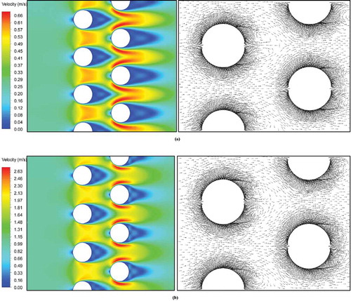
The flow field behavior across the collectors was assessed for inlet velocities of 0.25 m/s and 1 m/s. The 1 m/s velocity was chosen as it represented a common test velocity, while the 0.25 m/s velocity was arbitrarily chosen to compare the effects of velocity reduction. Figure 5 presents the visual description of the subdomain of interest and result extraction location for different parameters. The results of the velocity field distribution in Figure 6 show, in general, symmetric streamlines about the domain centerline. The behaviors of the fluid in the wake region behind the cylindrical collectors showed the presence of re-circulation vortices which are opposite in rotational direction, equivalent in size and symmetric about the collector’s centerline. This flow behavior was consistent for both collector rows (Collection Row 1 and Collection Row 2 as labeled in Figure 3).

Figure 5. Subdomain of interest and result locations

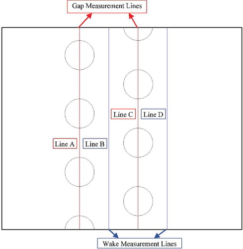
Figure 6. Comparison of velocity field distributions (as well as velocity vector plots) for flow across cross-flow cells (a) 0.25 m/s; (b) 1 m/s

Transverse velocity and turbulence intensity measurements across interstitial gaps

The results in Figure 7 show a non-dimensional value of the mean velocity and turbulence intensity measured across the transverse result lines in the interstitial gaps across the collector cells (see Figure 5). The results presented here utilized spatial coordinates in the transverse direction normalized by the transverse pitch length.

Figure 7. nondimensional transverse flow (simulation) profiles across interstitial gaps for normalized mean velocity (a) Gap velocity profile (simulation) results across Row 1(b) Gap velocity profile (simulation) results across Row 2 (c) Wake velocity profile (simulation) results across Row 1 (d) Wake velocity profile (simulation) results across Row 2

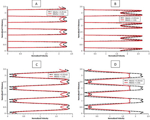
The velocities measured in Figure 7 were normalized by the respective inlet velocities and collected from transverse measurement lines (as shown in Figure 5), which quantified the flow behavior across the interstitial spaces. The maximum velocity (determined from the aforementioned measurement locations) showed an increase of 2.35 and 1.90 times the reference free-stream velocity (for the collection row 1, lines A and B) and an increase of 2.7 and 2.35 times the free-stream velocity (for collection row 2, lines C and D) for inlet velocity of 0.25 m/s. The tests at 1 m/s showed a similar increase of 2.35 and 1.85 times the reference free-stream velocity (for the collection row 1, lines A and B) and 2.5 and 1.80 times the reference free-stream velocity (for collection row 2, lines C and D). In all cases, the velocity increased downstream as it flowed over the second row of collector cylinders. Due to the staggered arrangements of the adjacent collector rows, the transversely measured mean velocity was anti-symmetric about the midpoint of the domain with full phase change to the orientation of the profile across the collector cells.

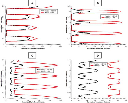
The measurements of turbulence intensity (Figure 8) across these gaps also provided useful information about the condition of the flow. Measurements taken between adjacent collectors (Gap Measurements Lines in Figure 5) on the same row showed (qualitatively) similar turbulence-velocity relationships (similar locations of maximum and minimum turbulence intensity in transverse direction) across both the first and second collection rows. The influence of the larger velocity on the turbulence intensity was most pronounced beyond measurement line A. The magnitude of turbulence intensity was maximum in the wake of the second collection row in both cases.

Figure 8. nondimensional transverse flow (simulation) profiles across interstitial gaps for normalized turbulence intensity (a) Gap turbulence profile (simulation) results across Row 1(b) Gap turbulence profile (simulation) results across Row 2 (c) Wake turbulence profile (simulation) results across Row 1 (d) Wake turbulence profile (simulation) results across Row 2

It should be noted that the behaviors observed under these flow conditions were independent of the applied electric field. Due to the diminished magnitude of the electric field in the region between discharge electrode and collector, in comparison to the regions between the anterior & posterior faces of the first and second row collection electrodes and the discharge electrodes, there was little or no effect of the electric field on the flow field.

Electric field distributions in cross-flow ESP

The ionic flux due to the convection and diffusion terms in Equation 3(3) $\overrightarrow{J}=b_i\left(q+q_p^c\right)\overrightarrow{E}+\left(q+q_p^c\right)\overrightarrow{u}-D_i\mathrm{\nabla }\left(q+q_p^c\right)$(3) had considerably less effects on the space charge distribution in comparison to the conductive term. For this reason, electric field distribution was independent of velocity conditions considered here. The distributions shown in Figure 9 are for the applied voltage of 70$\mathrm{k}\mathrm{V}$.

Figure 9. Electric field distribution in the collector zone of the cross-flow ESP for an applied voltage of 70 kV (a) X-component of local electric field distribution; (b) Y-component of local electric field distribution;(c) Magnitude of the local electric field distribution; (d) Global field distribution within the domain; (e) Charge density distribution at the electrode

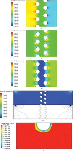
The electric field contours were densest around the wire surface with decreasing intensity toward the collector surface. The region with the dense electric field corresponded to the region of maximum voltage. The electric field contour lines took a circular shape close to the discharge electrode and distorted as they propagated toward the collectors. The space charge density was also maximum along the periphery of the discharge electrode with a value of approximately $1.87\mathrm{C}/{\mathrm{m}}^3$ and rapidly reduced in magnitude with increasing distance away from the discharge electrode. Most of the particle charging as well as electric force action was attained in the region closest to the electrode surface as that corresponded to the region with the densest electric field. The region between successive rows of the cross-flow cell showed a substantial difference in electric field magnitude in comparison to the regions outside that space. The field distribution was symmetric about the domain centerlines. Both rows showed varying magnitudes of electric field along the surface of the collector electrode, which is shown in Figure 9.

Collection mechanisms in cross-flow ESP

In this analysis, the particle trajectories and particle collection efficiency for various particle sizes ranging between 0.5 $\text{mum}$ and 10$\text{mum}$ were assessed under various turbulent inlet conditions with an inlet turbulent intensity of 5%. These values are typically encountered by ESPs in the field. A total of 350 stochastic particles were introduced and their trajectories were calculated using ANSYS Fluent’s DPM module along with the appropriate user-defined subroutines developed in this study to calculate the drag and electrical forces on the particles as it propagated through the flow stream.

The collection of particles was analyzed on two bases: firstly, the global path trajectory which described the path of deviation of the particle in the fluid stream when charged within the electric field as they approached the collector cell and secondly, the local particle collection across the collector array.

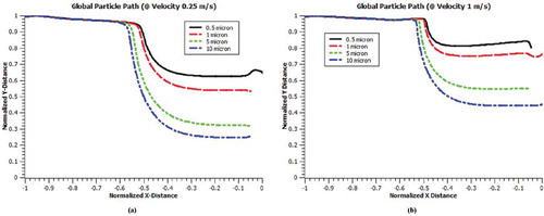
Figure 10 shows the global path of the particles in the stream after charging and upon approaching the collector cell. It is evident that given the similar order of magnitude of both electric field components, the lower flow velocities would result in larger deviations of the particle from the fluid flow path; with larger particle predictably deviating the most. This resulted in the utilization of fewer collectors in conditions of low enough free-stream velocities and generally higher collection efficiencies. Increasing free-stream velocity resulted in the global collection path tending closer toward the general flow path and for this reason, it was necessary to understand the collection across the cell.

Figure 10. Global particle trajectory in a cross-flow ESP with an applied voltage of 70 kV (a) 0.25 m/s; (b) 1 m/s

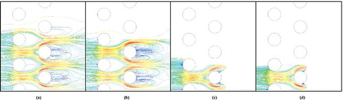
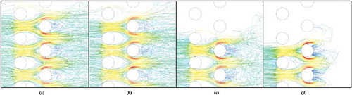
Figures 11 and 12 show collection across the cell for both (velocity) cases for the range of particles studied here. The trajectory colors represent the range in relative speed of the particles from blue (stagnant) to red (maximum). Each channel represents the flow path of the discrete particle size ranging from 0.5 microns to 10 microns. In each case, the location of the discharge electrode is at the top of the image (Figure 9d). The electric flux lines diverge outwards toward the extreme end of the model domain. For this reason, the electric field will have a greater effect on the motion of larger particles than the convective effects of the free stream. However, for smaller particles, this effect is not as pronounced, as the particles do not hold as much charge as the larger particles. This results in the larger particles (Figures 11d and 12d) to be transported further toward the domain boundary before reaching the collection electrodes as compared to the smaller particles (Figures 11a and 12a). Thus, collection of larger particles occurs on partial sections of the unit domain while smaller particles get collected on larger sections. This proves beneficial in comparison to traditional ESP’s since small particles in the center of the channel would most likely be carried through the flow without being collected on the parallel collection plates.

Figure 11. Local particle collection for inlet velocity of 0.25 m/s in a cross-flow ESP with an applied voltage of 70 kV (a) 0.5 μm; (b) 1 μm; (c) 5 μm; (d) 10 μm

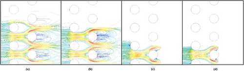
Figure 12. Local particle collection for inlet velocity of 1 m/s in a cross-flow ESP with an applied voltage of 70 kV (a) 0.5 μm; (b) 1 μm; (c) 5 μm; (d) 10 μm

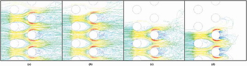
With respect to the regions of collection on the collector surface in all cases, the collection of particles corresponded to the positions of maximum electric field strength (Figure 9) along the surface of the collector. The particles were collected by two distinct means namely: impaction of the particles on the anterior surface of the first row and the collection on the posterior surface of the collectors in the staggered second row. In none of the cases did collection occur in the posterior of the first row or the anterior of the second row. The reason for this behavior, perhaps, rests in the flow characteristics across the interstitial spaces. The turbulence intensity in the gaps between the collector rows resulted in highly chaotic flow behavior and consequently in chaotic trajectories of the particle. This caused de-entrainment of particles within the flow and allowed the electric field in between to have a stronger influence on the particle’s trajectory. As the field charging is directly proportional to the square of particle’s diameter, the small particles collected very few charges. This was especially visible for particles under 1 µm. Due to this, increasing the electric field strength did not affect the smaller particle collection on the posterior of first row of electrodes and anterior of the second row of electrodes. On the other hand, the larger particles were easy to de-entrain at low mean velocities, but also carried more charge within the field. This allowed the large particle trajectory to be dictated almost exclusively by the intensity of the electric field in that region of low mean velocity.

In the region separating both rows of collectors, the turbulence intensity was quite low in the post-interstitial spaces as compared to the wake regions (in transverse direction) right behind the collectors. This resulted in the steady trajectory of the particles along with the fluid flow across the cell. This coupled with the negligible field strength in this region due to shielding by the collectors consequently did not favor collection within this region.

The results presented in Table 4 show the collection efficiencies estimates across a single cell. It shows that for particle as large as 5 $\text{mum}$ in this setup, higher velocities presented a challenge in collection. The collection behaviors, particularly, in the wakes of each collection row, provided insight into how this could be remedied. It is clear that the turbulence intensity distribution behind the collector rows was a major contributing factor to the collection of sub-micron particles. For this reason, it may be necessary to optimize the geometric definitions of the domain in order to induce high and evenly distributed turbulence behind all collector rows.

Table 4. Collection efficiency w.r.t particle size and inlet velocity

	Inlet velocity = 0.25 m/s	Inlet velocity = 1 m/s
0.5 $\text{mum}$	57.4%	25.14%
1 $\text{mum}$	86%	34.57%
5 $\text{mum}$	100%	80.57%
10 $\text{mum}$	100%	100%

Furthermore, the symmetry of the electric field distribution about the x-axis resulted in lower magnitudes of electric field in the gap between successive rows. In comparison to the velocity of the flow, these electric field magnitudes were neither high enough to force impaction on the anterior face of the second row of collectors nor retardation in the forward motion of the particle across this gap. Investigations into asymmetric arrangements of the discharge electrodes about the centerline of the collector cell, perhaps as a means of altering the field strength distribution in the separating gap, will be explored in future.

Experimental comparison

In order to validate model output presented above, experiments were conducted on the pilot cross-flow wet ESP system at Ohio University’s ESP laboratory as shown in Figure 13. The system consisted of an inlet, main chamber, and an outlet. A dust feeder was attached to the inlet, while the outlet was connected to a variable-frequency drive fan, capable of generating velocities up to 20 m/s. This inlet diffuser consisted of two perforated and four flow directional plates to assist in uniform inlet velocity profiles. The addition of these plates allowed for a more uniform velocity distribution and alleviated zones of inconsistent velocity. The main duct consisted of a single cell of collector electrodes comprising of two staggered rows of vertical collectors. The unit cell dimensions were 0.6 m wide, 1.8 m high and 0.0254 m thick. The collection electrodes were made with polypropylene rope and were grounded through a film of water produced by a steady supply of water from a water delivery system operating at 2.5 L/m³.

Figure 13. Cross-flow ESP experimental system

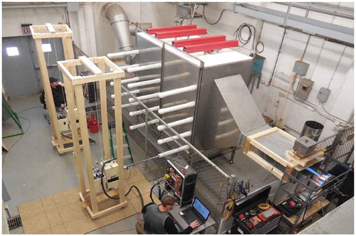
The voltage was applied to spiked discharge electrodes comprising of a 0.05 m diameter tube and a 0.089 m long spikes. The distance between each row of electrode tip and cell surface was 0.127 m, and between the two electrode tips in each row was 0.254 m. A Transformer-Rectifier unit, with a maximum capacity of 70 kV, was used to supply the voltage to the discharge electrodes. Figure 14 depicts the top view schematic of the experimental setup.

Figure 14. Cross-flow ESP experimental schematic (top view)

The average flow velocity during the test was controlled at 2.5 m/s at the test chamber inlet, while the particle concentration at the inlet was approximately 30 mg/m³. For a single cross-flow cell, the pressure drop across the cell was measured experimentally and through CFD analysis to be 25 Pa per cell. The voltage at the discharge electrode during the tests was maintained at an average steady state of 67 kV and 16 mA.

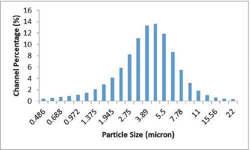
A particulate monitoring unit, ADR-1500, measured the particle mass concentration at the inlet and outlet instantaneously using light scattering photometry method as well as EPA Method 5. The measurements occurred at nine positions arranged in a 3-by-3 grid evenly spaced within the test chamber cross-section. This test array was performed before and after the cross-flow cell to measure capture efficiency. The particles introduced into the system had a distribution represented in Figure 15 with a mean particle size of 3.75 microns. These values were determined using Beckman Coulter LS 13 320 MW Particle Size Analyzer.

Figure 15. Particle size distribution used in the experimental study

The results of the experiments yielded a gross measured collection efficiency of 65–69%. The measured drop-out efficiency of the system without an applied voltage was estimated to be about 15%. This resulted in collection efficiency of 52 ± 2%.

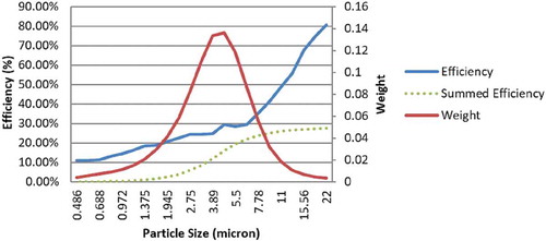
The numerical method previously described was utilized in assessing the collection efficiency of the configuration under the same conditions as the experimental analysis. The dimensions of the simulation were adjusted to match those of the experimental test. Additionally, flow velocity was increased from 1.0 m/s to 2.5 m/s to allow for direct comparison to experimental results. Figure 16 shows the results of the efficiency estimated numerically for each channel. Due to the distribution of the particle size, each channel contributed differently to the overall collection estimate. The reported efficiencies are number weighted comparing collection versus number of particles introduced per channel size. This was defined by a weighted efficiency for each particle size and was summed to provide the total gross efficiency (Summed Efficiency, Figure 16), which resulted in 28% bulk collection efficiency of the system. This result is lower than the experimental result of 52% which is due to factors (mentioned next) not included in the numerical model. The reasons for lower efficiency prediction by the proposed model are most likely due to the: 1) absence of any collection electrode vibration in simulation code 2) absence of mist formation due to water shedding, and 3) absence of high humidity resulting in particle agglomeration (74% – 77% humidity in the experiments). Albeit this difference, the proposed model provides critical information on flow, electric field distribution, and particulate collection efficiency for a range of particle sizes. The present work on cross-flow arrangement will be useful in developing cost-effective understanding of collection mechanisms for future tests of similar configurations.

Figure 16. Channel efficiency of simulation model for particle size distribution used in the experiment

Conclusion

In this study, a numerical modeling approach was developed to predict the collection behavior of a novel cross-flow ESP system. The simulation results showed that the electric field on either side of the pair of collector rows was dominant in particle collection, whereas, the weak field between each pair of rows produced negligible collection. For the model configuration presented, particle capture on the (collection) electrodes was limited to the anterior and posterior surfaces of the first and second rows, respectively. The collection at the posterior surface of the second row presented interesting behavior with the particles becoming entrained in the wake of the collectors as a result of the turbulence generated behind the collectors and the retardation force of the discharge electrode located downstream. The region separating the staggered electrodes presented no advantage in terms of collection. The electric field strength was weakest in this region and at high velocity the electric field’s influence on the particles trajectory within this region was minimal. When compared with the experimental data, the numerical approach presented here under predicted the collection efficiency. This was attributed to the limitations of the current model in accounting for collision and coalescence of particles, omission of any collection electrode vibrations and mist formation. Future work will aim to assess the effects of collector vibration on turbulence generation and its effects of particle coalescence. Despite differences with experimental data, the proposed numerical approach provides a cost-effective approach of gaining insight into the collection mechanism of the novel cross flow and other similar systems.

Acknowledgment

The authors would like to thank anonymous referees for providing useful, constructive, and insightful feedback that resulted in a significant improvement of the original manuscript.

Disclosure statement

No potential conflict of interest was reported by the authors.

Additional information

Funding

This work was completed through a grant provided by the Ohio Coal Development Office, a subsidiary of Ohio Development Services Agency, the State of Ohio, (GR 11375-10-1331570). The research was conducted in Ohio University’s Electrostatic Precipitator Laboratory, Athens, Ohio.

Notes on contributors

Ohioma Eboreime

Ohioma Eboreime is (Doctoral) Research Assistant in the Department of Mechanical Engineering at Ohio University, in Athens, OH, USA.

Muhammad Ali

Muhammad Ali is professors in the Department of Mechanical Engineering at Ohio University, in Athens, OH, USA.

Khairul Alam

Khairul Alam is professors in the Department of Mechanical Engineering at Ohio University, in Athens, OH, USA.

Alireza Sarvestani

Alireza Sarvestani is an Assistant Professor in the Department of Mechanical Engineering at Mercer University, in Atlanta, GA, USA.

Sean Jenson

Sean Jenson is (Doctoral) Research Assistant in the Department of Mechanical Engineering at Ohio University, in Athens, OH, USA.

References

- Alam, K., and H. Pasic. 2017. Wet electrostatic precipitator and method of treating an exhaust. US Patent US20170232450A1.
- Ali, M., H. Pasic, K. Alam, S. Tiji, N. Mannella, T. Silva, and T. Liu. 2016. Experimental study of cross-flow wet electrostatic precipitator. J. Air Waste Manage. Assoc. 66 (12):1237–44. doi:10.1080/10962247.2016.1209258.
- Altman, R., W. Buckley, and I. Ray. 2001. Wet electrostatic precipitation demonstrating promise for fine particulate control-part II. Power Eng. 105:42–44.
- Altman, R., G. Pepri, W. Buckley, and I. Ray. 2001. Wet electrostatic precipitation demonstrating promise for fine particulate control-part I. Power Eng. 105:37–39.
- ANSYS. 2015. ANSYS fluent theory guide. Canonsburg, PA: ANSYS, Inc.
- Chang, Q., C. Zheng, X. Gao, P. Chiang, M. Fang, Z. Luo, and K. Cen. 2015. Systematic approach to optimization of submicron particle agglomeration using ionic-wind-assisted pre-charger. Aerosol Air Qual. Res. 15 (7):2709–19. doi:10.4209/aaqr.2015.06.0418.
- Chang, Q., C. Zheng, Z. Yang, M. Fang, X. Gao, Z. Luo, and K. Cen. 2017. Electric agglomeration modes of coal-fired fly-ash particles with water droplet humidification. Fuel 200:134–45. doi:10.1016/j.fuel.2017.03.033.
- Chen, T., C. Tsai, S. Yan, and S. Li. 2014a. An efficient wet electrostatic precipitator for removing nanoparticles,submicron and micron-sized particles. Separation and purification technology 136:27–35.
- Chen, T., C. Tsai, S. Yan, and S. Li. 2014b. An efficient wet electrostatic precipitator for removing nanoparticles,submicron and micron-sized particles. Sep. Purif. Technol. 136:27–35. doi:10.1016/j.seppur.2014.08.032.
- Crawford, M. 1976. Air pollution control theory. USA: McGraw-Hill.
- Eboreime, O. 2019. Numerical modeling of the novel cross-flow electrostatic precipitator. Athens: Ohio University.
- Farnoosh, N., K. Adamiak, and G. Castle. 2011. Numerical calculations of submicron particle removal in a spike-plate electrostatic precipitator. IEEE Trans. Dielectr. Electr. Insul. 18 (5):1439–52. doi:10.1109/TDEI.2011.6032814.
- Feng, Z., Z. Long, and K. Adamiak. 2016. A critical review of models in numerical simulation of electrostatic precipitators. IAPGOS 6 (4):9–17. doi:10.5604/01.3001.0009.5182.
- Flagan, R., and J. Seinfield. 1988. Fundamentals of air pollution engineering. NJ: Prentice Hall Publication.
- Fujishima, H., Y. Ueda, K. Tomimatsu, and T. Yamamoto. 2004. Electrohydrodynamics of spiked electrode electrostatic precipitator. J. Electrost. 62 (4):291–308. doi:10.1016/j.elstat.2004.05.006.
- Gallimberit, I. 1998. Recent advancements in the physical modeling of electrostatic precipitators. J. Electrost. 43 (4):219–47. doi:10.1016/S0304-3886(98)00009-6.
- Haque, S. M. E., M. G. Rasul, M. M. K. Khan, A. V. Deev, and N. Subaschandar. 2007. A numerical model of an electrostatic precipitator. 16th Australasian Fluid Mechanics Conference, Goald Coast, Australia.
- Hautanen, J., M. Kilpelainen, E. Kauppinen, K. Lehtinen, and J. Jokiniemi. 1995. Electrical agglomeration of aerosol particles in an alternating electric field. Aerosol Sci. Technol. 22 (2):181–89. doi:10.1080/02786829408959739.
- Kanazawa, S., T. Ohkubo, Y. Nomoto, and T. Adachi. 1993. Submicron particle agglomeration and precipitation by using a bipolar charging method. J. Electrost. 29 (3):193–209. doi:10.1016/0304-3886(93)90024-2.
- Kaptzov, N. 1947. Elektricheskie invlentiia v gazakh i vakuumme. OGIZ 587–630.
- Laitinen, A., J. Hautanen, J. Keskinen, E. Kauppinen, J. Jokiniemi, and K. Lehtinen. 1996. Bipolar charged aerosol agglomeration with alternating electric field in laminar gas flow. J. Electrost. 38 (4):303–15. doi:10.1016/S0304-3886(96)00038-1.
- Nicol, K. 2013. Recent developments in particulate control. London, UK: IEA Clean Coal Center.
- Peek, J. W. 1929. Dielectric phenomena in high voltage engineering. New-York: McGraw-Hill.
- Versteeg, H., and W. Malalasekera. 2007. An introduction to computational fluid dynamics: The finite volume method. 2nd ed. Essex: Pearson Education Limited.
- Ye, Q., and J. Domnick. 2003. On the simulation of space charge in electrostatic powder coating with a corona spray gun. Powder Technol. 135-136:250–60. doi:10.1016/j.powtec.2003.08.019.