Operational bias correction for PM_2.5 using the AIRPACT air quality forecast system in the Pacific Northwest

ABSTRACT

A bias correction scheme based on a Kalman filter (KF) method has been developed and implemented for the AIRPACT air quality forecast system which operates daily for the Pacific Northwest. The KF method was used to correct hourly rolling 24-h average PM_2.5 concentrations forecast at each monitoring site within the AIRPACT domain and the corrected forecasts were evaluated using observed daily PM_2.5 24-h average concentrations from 2017 to 2018. The evaluation showed that the KF method reduced mean daily bias from approximately −50% to ±6% on a monthly averaged basis, and the corrected results also exhibited much smaller mean absolute errors typically less than 20%. These improvements were also apparent for the top 10 worst PM_2.5 days during the 2017–2018 test period, including months with intensive wildfire events. Significant differences in AIRPACT performance among urban, suburban, and rural monitoring sites were greatly reduced in the KF bias correction forecasts. The daily 24-h average bias corrections for each monitoring site were interpolated to model grid points using three different interpolation schemes: cubic spline, Gaussian Kriging, and linear Kriging. The interpolated results were more accurate than the original AIRPACT forecasts, and both Kriging methods were better than the cubic spline method. The Gaussian method yielded smaller mean biases and the linear method yielded smaller absolute errors. The KF bias correction method has been implemented operationally using both Kriging interpolation methods for routine output on the AIRPACT website (http://lar.wsu.edu/airpact). This method is relatively easy to implement, but very effective to improve air quality forecast performance.

Implications: Current chemical transport models, including CMAQ, used for air quality forecasting can have large errors and uncertainties in simulated PM_2.5 concentrations. In this paper, we describe a relatively simple bias correction scheme applied to the AIRPACT air quality forecast system for the Pacific Northwest. The bias correction yields much more accurate and reliable PM_2.5 results compared to the normal forecast system. As such, the operational bias corrected forecasts will provide a much better basis for daily air quality management by agencies within the region. The bias corrected results also highlight issues to guide further improvements to the normal forecast system.

Introduction

Air quality forecast systems based on chemical transport models typically have difficulty with accurate forecasts for PM_2.5 concentrations. The complexity and uncertainty of PM sources and particle dynamics present significant challenges for realistic simulations; our understanding of these processes in the atmosphere continues to be highly uncertain. The Air Indicator Report for Public Awareness and Community Tracking (AIRPACT) forecast system, which operates daily within the Pacific Northwest, uses emissions data obtained from local and state agencies together with meteorological fields generated using the Weather Research and Forecasting (WRF) model (Mass et al. 2003) as inputs to the Community Multiscale Air Quality (CMAQ) model (Chen et al. 2008; Herron-Thorpe et al. 2014; Vaughan et al. 2004). This system also includes automatic evaluation using local surface observations reported hourly via the AirNow system. While the system provides very useful results in terms of spatial patterns and forecast air quality index (AQI) categories, rigorous evaluation at individual monitoring sites indicate that forecast PM_2.5 concentrations have significant biases. Typical results for sites in urban Seattle include fractional bias (FB) as large as +75% in the winter and +25% in the summer, while performance for more rural sites varies from −25% in the winter to −50% in the summer and fall. Results at individual monitoring sites are generally worse during periods with regional wildfires in the late summer and early fall. The overall performance has not changed significantly even with several major upgrades in the modeling system over the past decade (Munson 2019). It is also true that there have been system shortcomings as well as upgrades. There were periods where daily updates to the chemical boundary conditions (BCON) were not available so monthly average BCON fields were used, and there were periods where significant changes in the wildfire location and emission processing caused issues during wildfire periods. Overall, however, the value of the system for daily air quality management does not meet its potential, and local agencies do not utilize the forecast system to the extent possible.

While it is important to continue to improve the modeling systems with better representations of emissions, atmospheric dynamics, and particle chemistry and physics, there are more immediate steps available to improve forecast skill and enhance the value of the forecasts for daily air quality management. Bias correction using available observations to correct model results is one approach that has been used in recent years. Initially, Delle Monache et al. (2006) demonstrated how a Kalman Filter scheme could be used to bias correct ozone levels in British Columbia. Kang et al. (2008, 2010a, 2010b) used the same approach as detailed by Della Monache to bias correct ozone (Kang, Mathur, and Rao 2010a; Kang et al. 2008) and then PM_2.5 (Kang, Mathur, and Rao 2010a, 2010b) for the US national air quality forecast system. Djalalova, Monache, and Wilczak (2015) and more recently Huang et al. (2017) have reported further efforts to implement bias correction for the national PM_2.5 forecast system. While Djalalova, Monache, and Wilczak (2015) assessed several methods, the best approach involved identification of PM_2.5 and weather analogs from training data sets and then Kalman filtering of observations to determine site-specific bias corrections. As described in Huang et al. (2017), these bias corrections were then interpolated using an iterative objective analysis scheme to adjust CMAQ grid values throughout the domain for each forecast time step. Overall forecast performance was improved, but the bias correction method still had issues with extreme events, such as wildfires. In China, a similar investigation was reported by Lyu, Zhang, and Hu (2017). These authors tested a number of different methods for each step in the bias correction process and found that a Classification and Regression Trees-Linear Model-Kalman Filter Analog combination worked best. In this approach, the classifier was used to select meteorological and pollutant factors that were most effective for the bias correction method and then a cluster analysis was applied using these factors to identify key analogs. Next, the Kalman filter was applied using the analogs to estimate the bias correction at each monitoring site, and the bias correction was interpolated to the model grids. While the method improved forecast performance, there were shortcomings due to the fact that emissions were changing rapidly enough during the 2014–2015 training period that the forecast periods in 2016 were affected by different emissions. Other studies have tested similar methods and generally found improved forecast performance with limitations due to extreme events or other non-constant conditions (Monteiro et al. 2013; Antonopoulos et al. 2014; Crooks and Ozkaynak 2014;; Silibello et al. 2015).

While the combination of machine learning and cluster analyses provides a good basis for determining bias correction, these methods also are more complicated than may be necessary to achieve good forecast performance. For that reason, in this paper, our objective was to develop a relatively simple approach using a Kalman Filter (KF) with suitable interpolation as the basis for an operational bias correction for the AIRPACT system. Our intent was to obtain significant improvements in the PM_2.5 forecast results while keeping the method simple and fast enough for daily forecast completion.

Methods

The AIRPACT forecast system

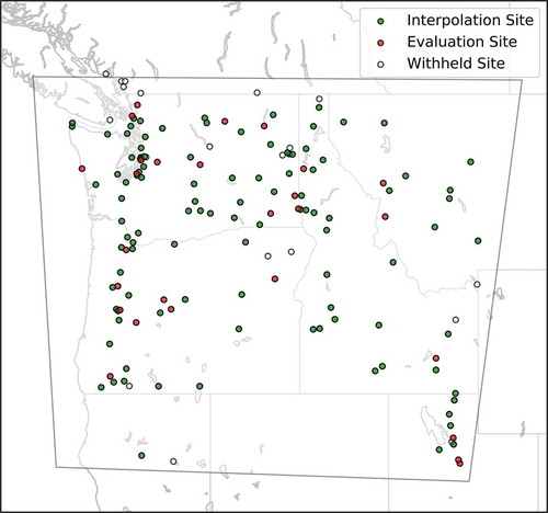
The AIRPACT system was initiated in 2001 (Mass et al. 2003; Vaughan et al. 2004; Chen et al. 2008; Herron-Thorpe et al. 2014, 2014b) and currently provides daily 48-h forecasts for Idaho, Oregon, Washington, and surrounding areas. The domain, shown in Figure 1, is a grid of 285 columns (E-W) by 258 rows (N-S) of 4 km x 4 km horizontal grid cells, with 37 variably spaced vertical layers from the surface to the 100-hPA pressure level. The gridded emission inventory, which is updated dynamically via SMOKE (Sparse Matrix Operating Kernel for Emissions, version 3.5.1) for the forecast day and weather conditions, is based on emissions data compiled by local and state agencies for the EPA National Emission Inventory (currently NEI, 2014). Mobile emissions are processed using the EPA mobile source emissions tool MOVES via SMOKE. Biogenic emissions are produced daily using the MEGAN (version 2.1) biogenic emission model (Guenther et al. 2012). Wildfire and prescribed fire emissions, including some agricultural burning, are obtained using the BlueSky Framework (Larkin et al. 2009) to acquire fire size and locations from SMARTFIRE (Raffuse et al. 2009), while emissions processing is streamlined through customized lookup tables and plume rise is calculated using the DEASCO3 method (Mavko and Morris 2013), which generates improved plume characterization. Chemical boundary conditions are obtained from the NCAR Whole Atmosphere Community Climate Model (WACCM; https://www.acom.ucar.edu/waccm/forecast/). Meteorological fields are obtained from the University of Washington’s WRF (version 4.1.3) forecasts produced each night (http://www.atmos.washington.edu/mm5rt/), and these are input via the Meteorological Chemical Input Processor (MCIP, version 5.1) to CMAQ (version 5.0.2, doi:10.5281/zenodo.1079898) for each air quality forecast simulation. The CMAQ results are processed to produce hourly PM_2.5, by summing appropriate aerosol species; a rolling 24-h average PM_2.5 product is also calculated. The most recent version is AIRPACT5, and the forecast products, including hourly meteorology, emissions, pollutant values in both map view and vertical curtain plots, on the domain boundaries and North-South and East-West on the interior of the grid, are made available as animations via the web at http://lar.wsu.edu/airpact/. As surface observations of PM_2.5 (see Figure 1) and other pollutants are reported via AirNow, these data are ingested and used to automatically produce performance evaluation statistics and time series graphs of forecast and observed results.

Figure 1. The AIRPACT forecast domain showing available AirNow PM_2.5 monitoring sites. Symbols: green, used for interpolation of bias; and red, used for evaluation of the interpolated bias. The open symbols along with the green and red symbols are the sites used for the operational KF bias correction system

Kalman filtering for biases at monitoring sites

Within the AIRPACT domain, there are approximately 130 sites with PM_2.5 monitors (see Figure 1), although the number varies over time. For the work reported here, we have used the AirNow data for the available sites as the basis for testing our methods and for the daily operations. While the data are quality checked in the AirNow system, the data have not been quality assured by the agencies as is the case for the EPA AQS data which is not available for several months after the observations are made. The monitors include both BAMs and nephelometer analyzers for PM_2.5, but we have not made any distinction here. While AirNow does not convey instrument type to data users on a per monitoring site basis, the network’s PM_2.5 monitors can be summarized as follows: For 2018, AirNow PM_2.5 instruments providing hourly (continuous) results for the US. included 579 Federal Equivalent Method (FEM) instruments plus 361 non-FEM instruments. The PM_2.5 instruments used for continuous data collection are, in order of prominence, Met One BAM (Beta Attenuation Mass Monitor, various models), Thermo beta attenuation instruments and TEOMs (tapered element oscillating microbalance), with the Teledyne T640 series gaining in usage share.

Our general approach involves using the PM_2.5 bias (forecast for grid cell minus observed at site) over an initialization window of time to compute the bias estimate for the forecast period. A Kalman filter is applied to the training time series window to determine a weighting factor for recent past bias to estimate current bias:

(1) $\mathrm{e}\mathrm{r}\mathrm{r}\mathrm{o}{\mathrm{r}}_{\mathrm{t}}=\left[1-\mathrm{e}\mathrm{r}\mathrm{r}\mathrm{o}{\mathrm{r}}_{\mathrm{t}-1}\right]K_t+{\epsilon }_t$(1)

where error_t is the predicted bias at time step t, error_t-1 is the actual bias between model forecast and observed PM_2.5 concentration at time step t-1, K_t is the Kalman gain, which is the optimal weighting factor that is determined in the training process, and ε_t is a noise term that is updated by the filter after setting an initial value. Delle Monache et al. (2006) provide details on the application of the Kalman filter method for air quality purposes. Kang et al. (2008, 2010a, 2010b) followed the same methodology. The error or bias term is used with the model output to calculate corrected PM_2.5 concentrations at each site for each forecast period:

(2) $\mathrm{m}\mathrm{o}\mathrm{d}\mathrm{e}{\mathrm{l}}_{\mathrm{c}\mathrm{o}\mathrm{r}\mathrm{r}\mathrm{e}\mathrm{c}\mathrm{t}\mathrm{e}\mathrm{d}}=\mathrm{m}\mathrm{o}\mathrm{d}\mathrm{e}{\mathrm{l}}_{\mathrm{r}\mathrm{a}\mathrm{w}}-\mathrm{e}\mathrm{r}\mathrm{r}\mathrm{o}{\mathrm{r}}_{\mathrm{t}}$(2)

where model_corrected is the hourly bias-corrected rolling 24-h averaged result for the site of interest and model_raw is the original hourly model 24-h rolling average forecast. Since PM_2.5 is managed on a 24-h averaged basis and to provide more data for initializing the KF method, we applied the KF method using hourly rolling 24-h average PM_2.5 concentrations at each site, but then evaluated and applied the method using daily 24-h averaged (midnight to midnight) PM_2.5 concentrations.

The above approach was used to explore the performance of Kalman filter bias correction at monitoring sites by using a multi-day training window to generate the Kalman gain and noise terms which are then used to predict the next day’s forecast bias at each monitoring site. Delle Monache et al. (2006) as well as Kang et al. (2008) used an initial 2-day training window and then accumulated training results through each successive modeling period. We tested both 7-day and 4-day windows and found no difference in the results; we adopted the 4-day window for training, but in our case, we re-initialized the KF filter with each successive 4-day window and did not accumulate training results over a longer period. We did this to minimize the influence of extreme events on following periods. We saw no difference in performance between re-initializing with a 4-day window or accumulating over a longer period.

In summary, we used the Kalman filter to produce an hourly time series of bias correction estimates for 24-h rolling average PM_2.5 concentrations for the forecast period, for each monitoring site. These bias values were applied as corrections to the corresponding AIRPACT forecast values at each site, and then the corrected daily 24-h (midnight to midnight) average PM_2.5 values were compared to the observed daily average at each site for each forecast day for 2017 and 2018 as described in Section 3. AIRPACT provides a 48-h forecast on a daily basis, but the bias correction scheme was applied only to the first 24-h of each forecast for test and evaluation purposes. The monitoring site bias corrections were interpolated to model grid points (described below) and the final KF products were daily maps of 24-h averaged PM_2.5 for the domain.

Interpolation of bias to the model domain

After the bias is calculated for 24-h average PM_2.5 concentrations at each site, these results can be interpolated to provide a map of biases that can be used to correct the forecasted 24-h average PM_2.5 concentration map. For interpolation of the biases at site locations to the model domain, we tested a cubic spline method and two Kriging methods. In a cubic spline interpolation, the resulting surface is fitted through the values at the points (sites) used in the interpolation. The curvature of the interpolated surface is minimized, resulting in a smooth surface. The cubic spline is a deterministic interpolation method, while Kriging is a geostatistical interpolation method which uses the autocorrelation of concentrations among sites. These interpolation approaches are representative of a variety of methods used in air quality observations and modeling (Deligiorgi and Philippopoulos 2011; Wong, Yuan, and Perlin 2004). Two Kriging interpolation methods, Gaussian and linear, were tested, with Gaussian and linear referring to the variogram model used in the interpolation. One obvious advantage of Kriging over cubic spline is that values are extrapolated in the area beyond the minimum polygon encompassing the sites used for interpolation. This means that grid cells on the edge of the domain receive a bias value for use in correcting the forecast. Results for the three interpolation schemes are presented in the Section 3.2.

Results and discussion

Bias correction at monitoring sites

For the initial tests of the bias correction, we used observed PM_2.5 AirNow data from 2017 to 2018 for approximately 130 monitoring sites within the AIRPACT domain (see Figure 1). The observed monthly averaged PM_2.5 concentrations averaged over all monitoring sites are shown in Figure 2 along with the corresponding raw AIRPACT Kalman filter corrected concentrations for the 2-year period. It is clear that the raw model forecasts underestimated observed concentrations for all months, except the wildfire month of September in 2017 and winter months in both years. In comparison, the bias-corrected concentrations were very close to the observed concentrations for all months.

Figure 2. Monthly averaged PM_2.5 concentrations for 2017 and 2018 observed and for the raw model and bias-corrected forecasts

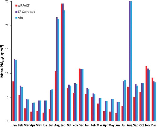
These monthly data averaged over the 2 years are summarized in Table 1 including the monthly averages of daily biases. Observed monthly averaged PM_2.5 concentrations were approximately 10 μg m⁻³ from November through February and near 5 μg m⁻³ during the spring, summer and late fall. However, very high observed 24-h PM_2.5 concentrations near 25 μg m⁻³ occurred in August (both years) and September (2017) as a result of extensive regional wildfires.

Table 1. Monthly average of daily biases [in %] for the raw model forecasts and for the Kalman filter bias correction method for 2017 and 2018

Month	Observed PM2.5 (μg m^−3)	Raw AIRPACT	Kalman filter
January	9.7	−25%	3%
February	6.4	−18%	3%
March	4.7	−32%	2%
April	4.1	−50%	−3%
May	4.5	−54%	−1%
June	4.2	−57%	0%
July	7.6	−62%	−3%
August	23.5	−62%	2%
September	15.3	−13%	6%
October	7.7	−14%	2%
November	9.2	−8%	4%
December	9.5	7%	1%
Average	8.9	−32%	1.3%

The raw forecast biases were almost always negative and in the range from −4% to more negative than −50%. Wintertime biases were somewhat less negative or even slightly positive, while the biases during the wildfire periods varied between +6% and −72%. In contrast, after bias correction using the Kalman filter, the biases were generally within ±6%, including the wildfire months (Table 1). Overall, the Kalman filter bias correction provided an immense improvement in model performance on a monthly averaged basis for all seasons.

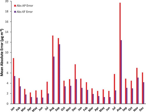
In addition to improving the bias in forecast PM_2.5 concentrations, the KF method also reduced the daily mean absolute errors (MAEs) on a monthly averaged basis as shown in Figure 3. For every month over the 2 years, the average daily MAE is larger for the raw forecast compared to the KF bias-corrected MAE. There are larger MAEs during the wildfire periods and during the winter for both the raw forecast and KF corrected values, which reflects more difficulty in simulating the intermittency and dynamics of wildfire plumes as well the complexities of wintertime stagnation periods. For wildfire periods, the MAE for the forecast ranges from 10 to 20 μg m⁻³, while the Kalman filter MAE ranges from 9 to 12 μg m⁻³. In the winter, the MAE is 5 to 8 μg m⁻³ for the raw model results and less than 5 μg m⁻³ for the Kalman filter results. In the summer, non-wildfire months, the MAE results are smaller and vary around 3 μg m⁻³ for the raw model results and even smaller for the Kalman filter results. Overall, it is clear the Kalman filter bias correction significantly decreases the absolute errors in the forecast.

Figure 3. Monthly averaged mean absolute error for the raw model forecasts and for Kalman filtering during 2017 and 2018

These improvements are similar to those reported in previous applications of the KF method for PM_2.5 forecast systems. Kang et al. (2010a) tabulated results that showed the normalized mean bias (NMB) averaged across different US regions was reduced from 24% to 12% and the normalized mean error (NME) was reduced from 59% to 39% during the cool season by using the KF bias-correction method. For the warm season, the NMB changed from −5% to +4%, and the NME was reduced from 46% to 34%. Djalalova, Monache, and Wilczak (2015) used a KF method for the US national forecast system to correct hourly PM_2.5 concentrations and found improvements of 65% in the mean absolute error. However, Lyu, Zhang, and Hu (2017) for a CMAQ forecast in China found only limited improvement in the forecast, but they attributed this to the fact that the evaluation covered a time period when emissions were rapidly changing such that the training and evaluation were affected by different emissions. Our results showed improvements in mean bias from −32% to +1%. Mean absolute error improved by approximately 50%. As a result, the simple method used in this work appears to yield results quite comparable to other KF methods.

Because the KF method is essentially extrapolating bias from the preceding time periods, it is possible for the bias-corrected results to exhibit some lag which does not capture step changes in concentrations due to a relatively sudden change in conditions. This would be a more significant problem for an hourly bias correction process, but it is much less of an issue for the present case where the primary products are daily 24-h average PM_2.5 concentrations. We examined the potential for this phase shift in the KF results and found that while there was sometimes a shift of a few hours in the rolling 24-h averages between observed and KF bias-corrected concentrations, this shift was much less obvious in the 24-h (midnight to midnight) daily values. Similarly, because of the 24-h rolling averaging involved, there were no distinct diurnal average patterns, on a monthly averaged basis, in the observations or the KF results.

For air quality management purposes, it is also worthwhile to examine the performance of the bias corrections at monitoring sites during worst-case pollution days. For this purpose, we first examined the PM_2.5 concentrations across all the monitoring sites for the top 10 worst PM_2.5 days, based on the domain averaged observed concentrations, during winter months (Dec to Feb) shown in Figure 4 and during the wildfire months (Aug to Sep) shown in Figure 5. For winter conditions, the mean bias and mean absolute error for the 10 worst days are significantly reduced compared to the raw AIRPACT model results. Only for the 8^th and 10^th worst days (Figure 4), did the model forecast have smaller bias and absolute error than the corrected forecast. For the other worst-case days, both the corrected MBs and MAEs are less than approximately 10%.

Figure 4. Observed 24-h average PM_2.5 concentrations across all sites during winter in 2017 and 2018 for the top ten highest PM days with associated mean biases (%) (top panel) and mean absolute errors (%) (bottom panel) for the AIRPACT raw and Kalman filtered bias-corrected forecasts

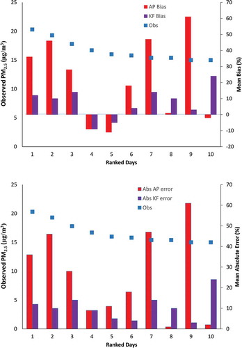
Figure 5. Observed 24-h average PM_2.5 concentrations across all sites during Aug and Sept (wildfire months) in 2017 and 2018 for the top ten highest PM days with associated mean bias (%) (top panel) and mean absolute errors (%) (bottom panel) for the raw AIRPACT and Kalman filtered bias-corrected results

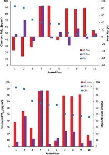
For the wildfire periods, where the maximum 24-h PM_2.5 concentrations reached 90 μg m⁻³, the AIRPACT biases and absolute errors were as large as 90% on five of the ten worst days, while the bias-corrected forecast only reached 90% errors on one day. On other days the errors in the bias-corrected forecast were less than 40% and on most days, less than 20%. This represents a valuable improvement for periods with highly intermittent and complex PM emissions and transport.

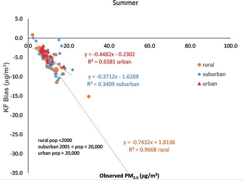
Seasonal differences are also apparent when the AIRPACT and Kalman filter bias are examined with respect to urban, suburban, and rural monitoring sites. For this case, the gridded population density was used to classify the type of site: urban with >20,000 people per grid cell, suburban with 2000 to 20,000 people per grid cell, and rural with <2000 people per grid cell. This classification is a simple way to categorize sites in terms of the density of human activities affecting PM emissions and concentrations. As shown in Figure 6, the magnitude of the Kalman filter bias averaged over winter months is distinctly different across the different site categories. For urban areas in winter, the AIRPACT model over-predicts PM_2.5 concentrations and the Kalman filter bias is positive. There is an urban to suburban to rural gradient in winter biases, from positive biases to very negative biases. As such, the Kalman filter bias results provide insight into issues with the AIRPACT simulations during winter. In highly populated areas, the PM_2.5 emissions, presumably from residential wood combustion, are overestimated, while in rural areas, sub-grid scale plume impacts may be missed by the model. This is reflected in the linear relationship between increasing negative bias and observed PM_2.5 concentrations. The same linear pattern exists for summer biases (Figure 7), but for summer the differences among site categories collapse to a single grouping of largely negative biases with increased under-prediction with increasing PM_2.5 concentrations. Since summer PM_2.5 peak concentrations are driven in part by wildfire impacts and not by population-related anthropogenic emissions, the type of monitoring site is not important, but the summer results show the need to improve treatment of wildfire dynamics and emissions in the model.

Figure 6. Kalman filter biases averaged for winter months (Dec-Feb) for each monitoring site versus the averaged winter PM_2.5 concentrations observed for each site, grouped by grid population density

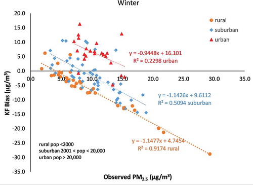
Figure 7. Kalman filter biases averaged for summer months (July-Sep) for each monitoring site versus the averaged summer PM_2.5 concentrations observed for each site, grouped by grid population density

The differences in AIRPACT and Kalman filter bias-corrected forecasts are also apparent in Figures 8 and Figures 9 which are Q:Q graphs of forecast and observed PM_2.5 concentrations.

Figure 8. Q:Q graph for the top ten worst PM days from 2017 and 2018 for rural sites during summer/early fall months

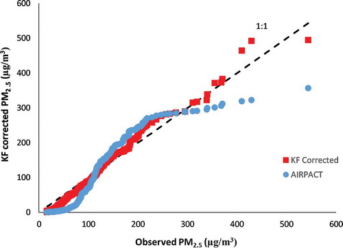
Figure 9. Q:Q graph for the top ten worst PM days from 2017 and 2018 for urban sites during winter months

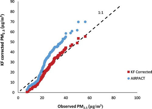
For summer/fall months at rural sites, which are often impacted by regional wildfires, the raw model results show a large under-prediction at relatively low concentrations (<100 μg m⁻³) and even more under-prediction at the high concentrations (>300 μg m⁻³). In contrast, the bias-corrected results fall close to the 1:1 line even at the highest observed concentrations.

For winter months (Figure 9) at urban sites where stagnation conditions can result in elevated PM concentrations, AIRPACT has a large over-prediction for the concentrations greater than 20 μg m⁻³. Again, the bias-corrected forecasts closely follow the 1:1 line over the entire concentration range except for the low concentrations (<20 μg m⁻³).

Overall, the evaluation of the Kalman filter bias correction at the monitoring sites shows that the bias correction greatly improves the model forecasts for both wintertime stagnation conditions and also for the more complex summer and fall wildfire periods.

Evaluation of spatially interpolated biases

To evaluate the interpolation schemes, bias corrections at 107 monitoring sites were interpolated to the model grid within the domain, while 24 sites were withheld from use in interpolation, for evaluation purposes (see Figure 1), including 11 rural sites, 9 suburban sites, and 4 urban sites. The withheld sites were randomly chosen within each site category. The interpolated bias results were used to correct the raw model 24-h average PM_2.5 for the entire grid, including those cells containing monitoring sites; these corrected results were then compared to the bias-corrected 24-h average PM_2.5 at those withheld sites.

Using 2017 as an example, monthly average MAE and MB after interpolation are summarized in Table 2. While there are variations in performance among the three methods on a monthly basis, overall the two Kriging methods appear to produce better results than the cubic spline approach, and these bias corrected and interpolated methods are better than the original AIRPACT forecasts. The Gaussian Kriging method yields a smaller bias, but a larger MAE, compared to the linear Kriging method. As a result, it is difficult to select one of the two Kriging methods as superior, although it appears the linear Kriging method might perform better during wildfire months since the MAE is lower and the MB is similar to the Gaussian Kriging method. It should also be noted that the interpolation introduces more bias and absolute error compared to the bias correction at individual sites without interpolation. For that reason, air quality managers may find the individual site bias-corrected results more useful for daily management decisions compared to the interpolated bias-corrected maps, while the maps will be useful for an overview of bias-corrected PM_2.5 concentrations throughout the domain.

Table 2. Monthly averaged Mean Absolute Error (MAE) and Mean Bias (MB) in μg m⁻³ for 24-h PM_2.5 concentrations for the original AIRPACT forecasts and the three bias-corrected interpolation methods. The mean bias-corrected PM_2.5 concentrations are also shown

		AIRPACT		Cubic Spline		Gaussian Kriging		Linear Kriging
Month	Bias Corrected PM2.5 (µg m^−3)	MAE	MB	MAE	MB	MAE	MB	MAE	MB
Jan-17	12.9	8.4	−4	9.0	3.1	6.0	1.1	5.3	1.9
Feb-17	7.4	4.1	−1.1	4.8	2.1	5.8	−0.4	3.6	1.7
Mar-17	4.6	2.7	−1.8	2.9	1.5	2.6	0.8	2.4	1.2
Apr-17	3.8	2.1	−1.6	2.2	1.5	2.0	0.4	1.7	0.6
May-17	4.3	2.7	−2.3	2.7	1.9	2.0	0.9	2.0	0.9
Jun-17	4.3	3	−2.6	2.5	1.8	2.4	0.3	2.0	0.7
Jul-17	6.5	4.7	−4.4	3.6	2.3	2.9	0.5	2.9	0.6
Aug-17	21.7	14.9	−11.6	16.3	0.2	12.5	1.6	9.0	2.2
Sep-17	24.5	13.8	−0.5	20.4	−7.5	13.2	3.3	12.2	3.5
Oct-17	7.6	4.2	0.3	4.7	2.0	3.6	1.2	3.4	1.5
Nov-17	8	4.2	−1	5.0	1.1	5.1	−1.0	3.5	1.4
Dec-17	10.9	6.9	1.5	9.0	3.3	6.3	2.7	5.7	3.6
AVERAGE	9.7	6.0	−2.4	6.9	1.1	5.4	0.9	4.5	1.6

The interpolation methods can also be compared in terms of the type of observation site: rural, suburban, or urban as shown in Table 3. For rural and suburban sites, the Gaussian method has a larger MAE, but a smaller MB compared to the linear method. For urban sites, however, both methods yield approximately the same ranges of MAE and MB.

Table 3. The bias-corrected PM_2.5 concentration and mean absolute error (MAE) and mean bias (MB) by site type for the two Kriging interpolation methods (µg m⁻³)

		Gaussian Kriging		Linear Kriging
Site Type	Bias Corrected PM2.5 (μg m^−3)	MAE	MB	MAE	MB
Rural	10.5	4.1	1.8	3.6	2.4
Suburban	9.3	3.1	0.8	2.7	1.4
Urban	8.5	3.1	2.0	3.0	1.8

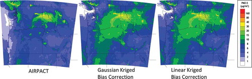
To illustrate the interpolation results for the Kriging methods, maps of bias-corrected 24-h average PM_2.5 concentrations are shown in Figure 10 for August 7, 2019 as an example day. In terms of the mapped results, it is difficult to distinguish differences between the two methods. Therefore, for operational use, daily maps for both Kriging methods are presented on the AIRPACT website.

Figure 10. Raw AIRPACT (left panel) 24-h average PM_2.5 and bias-corrected 24-h average PM_2.5 concentrations for August 7, 2019 using the Gaussian (center panel) and linear (right panel) Kriging methods for bias interpolation

Conclusion

In this work, a Kalman filter bias correction method has been developed and applied to the operational AIRPACT quality forecast system for 24-h average PM_2.5 concentrations. For individual monitoring sites, the bias-corrected results are significantly better than the raw AIRPACT forecast, both in terms of MAE and MB. This is also true for the top ten worst PM days during the 2017–2018 evaluation period. In operation, the bias correction method decreases the bias in 24-h average PM_2.5 concentrations from approximately −50% to ±6%. Mean absolute errors were also significantly decreased using the KF bias correction method. The AIRPACT system shows different levels of performance depending on the type of sites (rural, suburban, or urban), but the bias correction method generally improves the performance for all site types.

Three interpolation schemes were evaluated including a cubic spline method and Gaussian and linear Kriging methods. The Kriging methods were both better than the cubic spline method, but it was difficult to select one Kriging method as better than the other. The Gaussian method had smaller MB, but the linear method had a smaller MAE. Both Kriging methods have been included as routine web products for the operational bias correction scheme applied to the AIRPACT air quality forecasts.

Compared to the bias correction methods used by previous studies, the Kalman filter method developed in this study is a relatively simple method that is easy to implement and quick to compute. Despite being a simple approach, it shows a significant improvement in forecast performance. The improvement from the Kalman filter bias correction is much greater than the overall performance we achieved through several major upgrades in the modeling system over the past decade.

Acknowledgment

The authors thank Jill Schulte, Washington Department of Ecology, and Sara Strachan, Idaho Division of Environmental Quality, for their guidance and suggestions on interpolation methods and Ranil Dhammapala and Farren Herron-Thorpe, Washington Department of Ecology, for their helpful comments to improve the paper. This work was supported in part by the Northwest International Air Quality and Environmental Science & Technology (NW-AIRQUEST) consortium. The authors also acknowledge support from the National Science Foundation, Research for Experience for Undergraduates (AGS-1757711) summer program.

Disclosure statement

No potential conflict of interest was reported by the authors.

Additional information

Funding

This work was supported by the National Science Foundation [Research Experience for Undergraduates AGS-1757711]; NW-AIRQUEST Consortium.

Notes on contributors

Nicole June

Nicole June is a research assistant in the Department of Atmospheric Sciences at Colorado State University, Fort Collins, CO. She was previously an undergraduate student at Pennsylvania State University and participated in the NSF Research Experience for Undergraduates at WSU.

Joseph Vaughan

Joseph Vaughan is an Associate Research Professor in the Laboratory for Atmospheric Research and Department of Civil and Environmental Engineering at Washington State University, Pullman, WA.

Yunha Lee

Yunha Lee is an Assistant Professor in the Laboratory for Atmospheric Research and Department of Civil and Environmental Engineering at Washington State University, Pullman, WA.

Brian K. Lamb

Brian K. Lamb is Regents Professor Emeritus in the Laboratory for Atmospheric Research and Department of Civil and Environmental Engineering at Washington State University, Pullman, WA.

References

- Antonopoulos, S., J. Montpetit, V. Fortin, and G. Roy. 2014. Improving O3, PM2.5, and NO2 surface fields by optimally interpolating updatable MOS forecast, Chapter 40. In Air pollution modeling and its application XXII, ed. D. G. Steyn, Builtjes P., Timmermans R., 233–237. Dordrecht: NATO Science for Peace and Security Series C, Springer Science.
- Chen, J., J. Vaughan, J. Avise, S. O’Neill, and B. Lamb. 2008. Enhancement and evaluation of the AIRPACT ozone and PM2.5 forecast system for the Pacific Northwest. J. Geophys. Res. 113:D14305. doi:10.1029/2007JD009554.
- Crooks, J. L., and H. Ozkaynak. 2014. Simultaneous statistical bias correction of multiple PM2.5 species from a regional photochemical grid model. Atmos. Environ. 95:126–41. doi:10.1016/j.atmosenv.2014.06.024.
- Deligiorgi, D., and K. Philippopoulos. 2011. Spatial interpolation methodologies in urban air pollution modeling: Application for the greater area of metropolitan Athens, Greece. In Advanced air pollution, ed. F. Nejadkoorki, 341–362. IntechOpen. doi:10.5772/17734.
- Delle Monache, L., T. Nipen, X. X. Deng, Y. M. Zhou, and R. Stull. 2006. Ozone ensemble forecasts: 2. A Kalman filter predictor bias correction. J. Geophys. Res. Atmos. 111 (D5):D05308. doi:10.1029/2005JD006311.
- Djalalova, I., L. D. Monache, and J. Wilczak. 2015. PM2.5 analog forecast and Kalman filter post-processing for the community multiscale air quality (CMAQ) model. Atmos. Environ. 119:431–42. doi:10.1016/j.atmosenv.2015.05.057.
- Guenther, A. B., X. Jiang, C. L. Heald, T. Sakulyanontvittaya, T. Duhl, L. K. Emmons, and X. Wang. 2012. The model of emissions of gases and aerosols from nature version 2.1 (MEGAN2.1): An extended and updated framework for modeling biogenic emissions. Geosci. Model Dev. 5 (6):1471–92. doi:10.5194/gmd-5-1471-2012.
- Herron-Thorpe, F. L., G. H. Mount, L. K. Emmons, B. K. Lamb, D. A. Jaffe, N. L. Wigder, S. H. Chung, R. Zhang, M. D. Woelfle, and J. K. Vaughan. 2014. Air quality simulations of wildfires in the Pacific Northwest evaluated with surface and satellite observations during the summers of 2007 and 2008. Atmos. Chem. Phys. 14 (22):12533–51. doi:10.5194/acp-14-12533-2014.
- Huang, J. J., M. J. Wilczak, I. Djalalova, I. Stajner, P. Shafran, D. Allured, P. Lee, L. Pan, D. Tong, H. C. Huang, et al. 2017. Improving NOAA NAQFC PM2.5 predictions with a bias correction approach. Weather and Forecasting. doi:10.1175/WAF-D-16-0118.1.
- Kang, D., R. Mathur, and S. T. Rao. 2010a. Real-time bias-adjusted O3 and PM2.5 air quality index forecasts and their performance evaluations over the continental united states. Atmos. Environ. 44 (18):2203–12. doi:10.1016/j.atmosenv.2010.03.017.
- Kang, D., R. Mathur, and S. T. Rao. 2010b. Assessment of bias-adjusted PM2.5 air quality forecasts over the continental United States during 2007. Geosci. Model Dev. 3 (1):309–20. doi:10.5194/gmd-3-309-2010.
- Kang, D., R. Mathur, S. T. Rao, and S. Yu. 2008. Bias adjustment techniques for improving ozone air quality forecasts. J. Geophys. Res. 113 (D23):D23308. doi:10.1029/2008JD010151.
- Larkin, N. K., S. M. O’Neill, R. Solomon, S. Raffuse, T. Strand, D. C. Sullivan, C. Krull, M. Rorig, J. Peterson, and S. A. Ferguson. 2009. The bluesky smoke modeling framework. JOUR. Int. J. Wildland Fire 18 (8):906. doi:10.1071/WF07086.
- Lyu, B., Y. Zhang, and Y. Hu. 2017. Improving PM2.5 air quality model forecasts in China using a bias-correction framework. Atmosphere 8 (12):147–62. doi:10.3390/atmos8080147.
- Mass, C.F., M. Albright, D. Ovens, R. Steed, E. Grimit, T. Eckel, B. Lamb, J. Vaughan, K. Westrick, P. Storck, B. Coleman, C. Hill, N. Maykut, M. Gilroy, S. Ferguson, J. Yetter, J. M. Sierchio, C. Bowman, D. Stender, R. Wilson, and W. Brown. 2003. Regional environmental prediction over the Pacific Northwest, Bulletin Amer. Meteorol. Soc. 84, 1353–1366.
- Mavko, M., and R. Morris. 2013. DEASCO3 project updates to the fire plume rise methodology to model smoke dispersion. Denver, CO: Technical Memorandum, Air Sciences, Inc. https://deasco3.wraptools.org/.
- Monteiro, A., I. Ribeiro, O. Tchepel, E. Sa, J. Ferreira, A. Carvalho, V. Martins, A. Strunk, S. Galmarini, H. Elbern, et al. 2013. Bias correction techniques to improve air quality ensemble predictions: Focus on O3 and PM over Portugal. Environ. Model Asses. doi:10.1007/s10666-013-9358-2.
- Munson, J. A., 2019. Decadal evaluation of the AIRPACT regional air. quality forecast system in the Pacific Northwest from 2009-2018. M.S. thesis, Washington State University.
- Raffuse, S. M., D. A. Pryden, D. C. Sullivan, N. K. Larkin, T. Strand, and R. Solomon. 2009. SMARTFIRE algorithm description. JOUR. US Environmental Protection Agency, Research Triangle Park, NC, by Sonoma Technology, Inc., Petaluma, CA, and the US Forest Service, AirFire Team, Pacific Northwest Research Laboratory, Seattle,WA STI-905517-3719.
- Silibello, C., A. D’Allura, S. Finardi, A. Bolignano, and R. Sozzi. 2015. Application of bias adjustment techniques to improve air quality forecasts. Atmos Pollut. Research 6 (6):928–38. doi:10.1016/j.apr.2015.04.002.
- Vaughan, J., B. Lamb, R. Wilson, C. Bowman, C. Figueroa-Kaminsky, S. Otterson, M. Boyer, C. Mass, M. Albright, J. Koenitg, et al. 2004. A numerical daily air-quality forecast system for the Pacific Northwest. Bulletin Amer. Meteorol. Soc. 85:549–61. doi:10.1175/BAMS-85-4-549.
- Wong, D. W., L. Yuan, and S. A. Perlin. 2004. Comparison of spatial interpolation methods for the estimation of air quality data. J. Expo. Anal. Environ. Epidemiol. 14 (5):404–15. doi:10.1038/sj.jea.7500338.