Methane emissions from above-ground natural gas distribution facilities in the urban environment: A fence line methodology and case study in Calgary, Alberta, Canada

ABSTRACT

The occurrence and emissions of methane (CH₄) from above-ground urban natural gas infrastructure is poorly understood. Compared to below-ground infrastructure, these facilities are relatively easy to monitor and maintain and present an opportunity for cost-effective CH₄ reductions. We present a case study and methodology for detecting, attributing, and quantifying CH₄ emissions from fence line measurements at above-ground natural gas facilities in the City of Calgary, Alberta, Canada. We produced bounding-box concentration maps by walking around the outer fence of 33 facilities with a backpack-configured trace gas analyzer and a tablet with integrated GPS. Wind measurements were acquired simultaneously from a fixed location on site with a 3D sonic anemometer. We fused geolocation, CH₄ concentration, and wind data to determine the likelihood each facility was emitting. We found one definitive leak by carrying out measurements directly alongside an exposed section of pipe. Based on the presence of methyl mercaptan (CH₃SH) odor, peak ΔCH₄, and the difference between downwind and upwind ΔCH₄, we interpret a high plausibility that 22 facilities were emitting CH₄, followed by 2 with a medium plausibility, and 8 with a low plausibility. Once verified to plausibly emit, these data were used to estimate emissions flux at six facilities where near-field obstructions were limited. The estimated emissions flux for six facilities was 66.31 mg CH₄ s⁻¹, or 2.1 tonnes CH₄ yr⁻¹ if this flux remained constant. Overall, this study indicates most above-ground natural gas facilities surveyed in Calgary were emitting CH₄. These facilities represent easy mitigation targets for reducing CH₄ emissions and improving environmental performance. To our knowledge, this is the first study to integrate qualitative and quantitative information to predict detection plausibility in a complex measurement setting.

Implications: The fence line methodology outlined in this study represents an extension of source assessment modes in the US EPA’s Other Test Method 33A for human portable systems. This has implications for standardization of emissions measurement in situations where other platforms (e.g., vehicles) are less effective due to access limitations. We believe the methodology presented could become a recognized standard based on performance from controlled testing and added to the regulatory toolkit for emissions verification and compliance.

Introduction

In the past decade, atmospheric methane (CH₄) has garnered more attention from scientists and governments due to increasing awareness of its effect as a short-lived climate pollutant (Pierrehumbert 2014). This has prompted commitments to reduce emissions from several industries. Notably, the oil, gas, and coal sectors are being targeted for CH₄ reductions because they are one of the largest anthropogenic sources of emissions. As the principal component of natural gas is CH₄, there is further economic incentive for industry to address leaks throughout the supply chain and retain profitable gas (IEA, 2020). Natural gas has been marketed as an affordable, reliable, and cleaner fossil fuel that can play a critical role in a low-carbon future because it emits less carbon dioxide (CO₂) per unit of energy than coal or oil when combusted (Howarth 2014). However, when CH₄ from natural gas production, transmission, or distribution is directly released into the atmosphere through leaks or vents, it traps heat with a global warming potential (GWP) 84 times greater than CO₂ over 20 years and 28 times that of CO₂ in a 100-year time period (Myhre et al. 2013). This is significant because direct CH₄ emissions from any part of the natural gas supply chain can undermine their climate benefit (Alvarez et al. 2012).

Like upstream and midstream sectors (Alvarez et al. 2018), research on the downstream sector of the natural gas supply chain indicates that urban areas may be a larger source of CH₄ than inventories suggest (e.g., Klausner et al. 2020; Lamb et al. 2016; McKain et al. 2015; Plant et al. 2019; Ren et al. 2018; Wunch et al. 2016). For example, the average fractional loss rate for the downstream part of the natural gas supply chain in Boston, MA, was estimated at 2.7%, compared to best estimates for inventory losses of ~1.1% (McKain et al. 2015). This loss rate equates to ~$90 million annually in lost product for distribution companies in Boston (McKain et al. 2015). Losses of this magnitude and the associated climate impact suggest further research is warranted to better characterize the problem and guide the deployment of new abatement solutions.

Leaks from downstream natural gas infrastructure such as pipelines, gate stations, and metering and regulation (M&R) facilities are an important source of urban CH₄ emissions, along with those from other anthropogenic activities such as agriculture, landfills, and wastewater treatment. Greater interest has emerged in detecting and quantifying levels of urban CH₄ emissions linked to natural gas distribution to determine the contributions of downstream activities to the GHG footprint of the entire supply chain (Hendrick et al. 2016; Hopkins et al. 2016; Jackson et al. 2014; Lamb et al. 2015, 1995; McKain et al. 2015; Plant et al. 2019; von Fischer et al. 2017; Weller, Hamburg, and von Fischer 2020). However, this existing work does not sufficiently address the role of above ground natural gas infrastructure and commonly lacks the spatial and temporal resolution to guide leak detection and repair. In contrast, emissions from below-ground distribution systems are better studied, particularly in cities with old, leak-prone cast iron or bare steel underground pipelines (Hendrick et al. 2016; Phillips et al. 2013; von Fischer et al. 2017; Weller, Hamburg, and von Fischer 2020). While important, these sources tend to be expensive to repair (von Fischer et al. 2017). Fewer studies have examined emissions from above-ground urban natural gas infrastructure (e.g., gate stations, M&R facilities) where components are accessible and can be directly inspected, repaired, or retrofitted at lower cost than subsurface infrastructure (although see Lamb et al. 2015, 1995).

In this study, we build on past research to better resolve above-ground sources of CH₄ emissions downstream in the natural gas supply chain. The study involved fence line surveys at 33 above-ground natural gas distribution facilities in the City of Calgary, Alberta, Canada. The natural gas company that operates the facilities was not notified in advance of our activities. We used a backpack-configured trace gas analyzer to measure CH₄ concentration and combined those data with GPS coordinates and wind measurements at each facility. By walking facility perimeters with the backpack system, we adapted protocols outlined in the U.S. Environmental Protection Agency’s Other Test Method 33A (OTM33A: Thoma and Squier 2014) to map and attribute CH₄ sources and quantify emissions.

Methodology

Overview

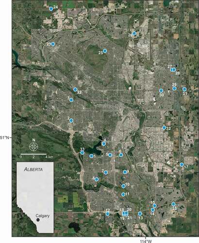
We surveyed 33 above-ground natural gas control and gate facilities in the City of Calgary between 25 May and 5 June 2020 (Figure 1). Gate facilities meter and regulate the gas pressure before it enters the city distribution system and odorize gas with mercaptan for safety. Control facilities operate within the city distribution system and further meter and regulate the pressure and flow of natural gas to consumers. Additional details on equipment functionality at these sites were unavailable as these surveys were conducted without knowledge of the operator. Most facilities in this case study were adjoining residential areas and easily accessible by foot. We note that our sample is not exhaustive of all facilities in the City of Calgary. Each site was visited once. Further, we were unable to determine if the facilities were pressurized and operating at the time of the survey.

Figure 1. Locations of natural gas gate and control facilities surveyed in this study

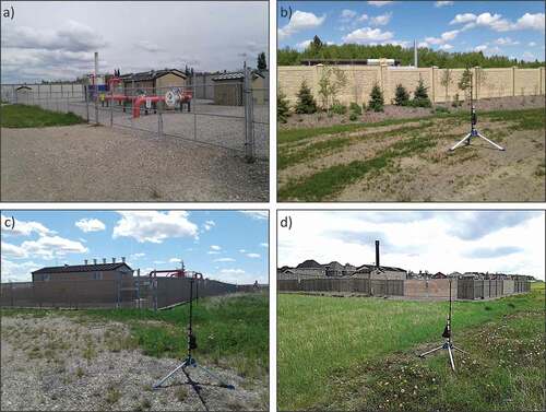
The configuration of above-ground equipment and fencing at each facility varied. Typical facilities had large diameter pipe and associated components exposed at the surface and one or more buildings housing additional equipment. Facility footprints ranged from 20 m² to over 15,000 m². Some facilities were enclosed by solid brick or wooden walls >3 m tall, while others were enclosed by 2 m tall chain link fencing, chain link fencing with slats, or a mix of two or more fencing types (Figure 2). Different fencing types or porosities affect how the gas mixes and disperses downwind, which limited our ability to acquire top-down emission rate estimates from most facilities.

Figure 2. Examples of different fencing around facilities. (a) This facility had chain link fencing on the north side, and ~3 m tall solid walls around the east, west, and south sides (note residential area in background). (b) A solid wall ~3 m tall around a gate facility. (c) Chain link fencing with slats. (d) A mix of ~2 m tall chain link fencing with slats and wooden fencing (note residential area in background). The anemometer tower in the foreground of (b)-(d) is 1.65 m tall

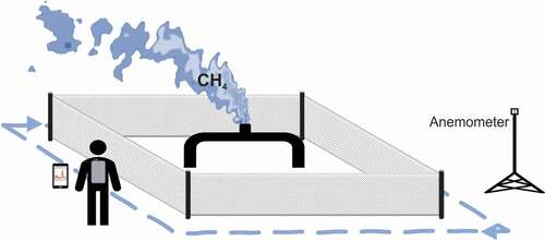
We measured CH₄ mixing ratio at each facility by walking outside the perimeter fence with a portable backpack trace gas analyzer, recording the position of each gas concentration measurement with a GPS-enabled tablet, and simultaneously measuring wind conditions from a fixed location nearby (Figure 3). This approach is similar to that used by Chen et al. (2020); the operator creates a bounding box of CH₄ measurements around facilities linked with wind data. It also emulates vehicle-based assessment modes in the U.S. Environmental Protection Agency’s (EPA) OTM33A (Thoma and Squier 2014): concentration mapping and source characterization. Resolving component-level emissions sources would have required close-range methods and coordination with the natural gas distribution company to gain facility access. We did, however, independently measure facility-level emissions under typical operating conditions without operator knowledge, limiting potential for bias.

Figure 3. Illustration of survey methodology using a portable backpack trace gas analyzer, GPS, and stationary anemometer

We estimated emissions rates for selected facilities by adapting protocols from OTM33A. The method requires an anemometer and a sensor that measures methane concentrations. For typical emissions quantification with OTM33A, the sensors are located 20–200 m downwind within the plume of a known emitting source. The method relies on ~20 minute periods of stationary and co-located CH₄ and wind measurements during which the natural variability of the wind allows the plume and its associated CH₄ concentrations to be assessed. OTM33A is a screening method for quantification that is used to triage follow-up activities. The biggest limiting factor for OTM33A emissions quantification measurements in this study was the presence of near-field obstructions, particularly the common occurrence of solid fences around facilities, which act as windbreaks and have the effect of suppressing near field concentrations. Accordingly, measurements to estimate emissions rates were acquired at 6/33 facilities with chain link fencing along the downwind perimeter.

Equipment

CH₄ concentration measurements were acquired with a LI-COR LI-7810 trace gas analyzer secured to a backpack. The analyzer uses optical feedback-cavity-enhanced absorption spectroscopy to measure CH₄, CO₂, and H₂O in the air. Air is drawn into the cavity by a small pump. Operators were screened to verify they did not exhale CH₄ prior to conducting surveys by breathing directly into the air intake, eliminating any potential for measurements to be high biased by the user’s breath. Measurements of CO₂ and H₂O were not considered in this study because they were contaminated by exhalations during the surveys. The LI-7810 measures CH₄ mixing ratio from 0.1 to 100 ppmv with a precision of 0.60 ppbv at 2 ppmv with 1 s averaging. The measurement rate and height were 1 s and 1.52 m, respectively. We noted a small drift in the LI-7810 internal clock before the study was undertaken, which was addressed each day by setting the clock relative to the time on a tablet that was used to configure the LI-7810 analyzer and display concentration data in real time via Wi-Fi connection. The tablet was a Samsung Galaxy Tab E with GPS + GLONASS. In addition to interfacing with the LI-7810 analyzer, the tablet was also used to collect the geolocation data. We used an app (Avenza Maps) to record survey tracks for each facility at a measurement rate of 1 Hz. We noted a 2 second offset between the tablet time and the GPS time, which was corrected during post-processing by shifting the GPS data series.

A TriSonica Mini 3D ultrasonic anemometer was used to measure wind components at each facility during the walking surveys. Where possible, the anemometer was positioned in an opening 10–20 m away from the facility and mounted 1.65 m above ground level on a small tripod. The measurement rate was 1 s. Data were recorded on a microSD card on the datalogger. Wind data were not recorded at six facilities due to a loose wire connection, which was corrected in subsequent surveys. To supplement missing on-site wind data, we used average hourly wind speed and direction from a weather station at the Calgary International Airport (World Meteorological Organization ID: 71877).

Daily procedures

Before each survey, the LI-7810 was initialized indoors at room temperature and warmed up for at least 35 minutes according to the manufacturer’s specification. The LI-7810 ran continuously until the last survey of the day was completed. The internal clocks of the LI-7810 and TriSonica were manually adjusted at the beginning of each day to match the time on the tablet to the nearest second. The clocks were also checked after the last facility survey was completed. We noted that the clocks drifted in the LI-7810 and TriSonica by less than 1 s over 5 hours. We estimate the relative time synchronization of all three data series was ~ 1 s.

After arriving onsite, the TriSonica was mounted on a small tower on level ground and its orientation was set to true north using a handheld compass (estimated accuracy of ±5°). Power was then supplied via USB cable connected to a small power bank. The mapping App was initialized, and GPS tracking was started. The surveys involved walking around each facility at least 3 times at a slow-to-moderate walking pace. Additional observations were made after each survey to contextualize emissions based on the following details: fencing characteristics, photographs, presence/absence of detectable odors of methyl mercaptan (CH₃SH), and the presence of other potential near-field sources of CH₄ emissions. Post-processing involved downloading and fusing data series from each sensor and correcting for known time offsets.

Plausibility of CH₄ emissions

To improve the accuracy with which CH₄ emissions were attributed to above-ground natural gas facilities, we established a plausibility approach that uses site level quantitative and qualitative data and is based on three binary criteria: (1) Methyl mercaptan (CH₃SH) odor (yes/no), (2) CH₄ concentration enhancements (ΔCH₄) >100 ppbv (yes/no), and (3) downwind ΔCH₄ 95^th percentile > upwind ΔCH₄ 95^th percentile (yes/no). We define a high plausibility a facility is emitting if the response is “yes” to all three criteria, followed by a medium plausibility if the response is “yes” to two criteria, and a low plausibility if the response if “yes” to one criterium or “no” to all three.

Methyl mercaptan is an organosulfuric compound added to natural gas with a distinct odor to facilitate human olfactory detection. During surveys, the operator recorded if they were able to smell CH₃SH at individual facilities. In this case, the operator had experience identifying CH₃SH odor, enabling them to distinguish it from any other atmospheric odors that may have been present at the location from upwind sources.

To account for spatial and daily variations of ambient CH₄, we used the 5^th percentile of concentration measurements at each facility to determine CH₄ concentration background, which is consistent with OTM33A and related research (Brantley et al. 2014; Sanchez et al. 2018; Thoma and Squier 2014). Based on this approach, the background mixing ratio ranged from 1932.5 to 1977.9 ppbv during the field campaign. Concentration enhancements (ΔCH₄) were derived by taking the difference between the CH₄ mixing ratio measurements and the 5^th percentile background levels at each facility.

As part of the last criteria of our emissions plausibility approach, we used geocoded CH₄ measurements, wind direction, and a Geographic Information System (ArcGIS Professional) to separate the data into upwind and downwind groups. The premise is that downwind ΔCH₄ should be higher at emitting facilities compared to the upwind ΔCH₄, whereas there should be little difference between the downwind and upwind ΔCH₄ at non-emitting facilities. Accordingly, we grouped concentration measurements based on the wind direction. First, we established a center point at each facility to base the analysis. We assumed the wind direction at the nearby anemometer approximated the wind direction at the center of the facility. At each 1 s timestep in the wind direction data, we determined if a concentration measurement was positioned downwind or upwind from the facility center point. To increase the sample size and account for spatial variations of the wind direction and arrangement of equipment and structures inside the fenced areas, we included concentration measurements ±25° in the upwind and downwind directions from the facility center point. Similarly, the ±25° wedge of upwind and downwind concentration measurements is large enough to incorporate small-scale disturbances in the local wind direction from turbulence generated by structures within the facility. For facilities with missing on-site wind data, we used a constant wind direction from hourly data recorded by a weather station at the Calgary International Airport. We calculated the 95^th percentiles of the downwind and upwind ΔCH₄ groups and determined the difference for each facility.

Quantifications

After completing the walking survey at each facility, we determined if near-field obstructions, non-target emissions sources, topographic features, and downwind access were within acceptable limits for emissions quantification (EQ) measurements based on the protocols outlined in OTM33A (Thoma and Squier 2014; see also Edie et al. 2020; Heltzel et al. 2020). Only six emitting facilities were deemed suitable. For those facilities, we determined the location of the plume from the walking survey and re-positioned and re-oriented the anemometer tower in line with the plume. We stood 1 m in the crosswind direction from the tower to collect CH₄ concentration measurements for 15 minutes. The upwind distance to the nearest equipment unit inside the fence line was estimated. We note that if a conventional, vehicle-based OTM33A EQ methodology were used, none of the facilities would have been suitable because they lack or have limited downwind road access.

Once data were collected, they were input into the EPA’s OTM33A Matlab® program (v. 1.3). This program bins mean CH₄ concentrations from paired 10° wind direction bins and creates a best-fit gaussian curve. Following protocols, data were rotated so that the bin with the highest concentration was associated with the 180° bins. At one of the six facilities we noted two distinct plumes and conducted separate OTM 33A measurements for each. The emissions estimates were summed to provide a facility flux.

In addition to the quantification, we used the worksheet in Appendix I of the OTM 33A documentation to calculate the composite Data Quality Indicator (DQI) score for each set of measurements. The composite DQI score is a sum of “points” from individual DQI criteria calculated from the data. Low composite DQI scores were generally associated with lower-error quantification estimates in controlled release testing (Thoma and Squier 2014). Critical DQIs include the fit of the Gaussian curve to the data (where points are assigned for R < 0.95), low methane mixing ratios (if peak above-ambient values are <0.15 ppmv), weak mean winds (<1.5 m/s), and several other factors (Thoma and Squier 2014). A DQI “flag” is associated with any quantifications whose DQI value > 8. In controlled emissions tests, DQI flags were shown to be associated with high-error quantifications.

Results

Olfactory detections

We detected methyl mercaptan (CH₃SH) odor at twenty-three facilities (Table 1), which is a strong indication these facilities were emitting CH₄. Generally, we detected CH₃SH odor when CH₄ mixing ratios exceeded 2000 ppbv. At eight facilities, the odor was also detected from sidewalks, alleys, and pathways up to 93 m downwind. In every case, no CH₃SH odor was detected upwind of the facilities.

Table 1. Summary statistics for each facility. Wind metrics include the mean wind speed ($\bar{u}$), resultant wind direction (θ_R), and wind direction standard deviation (${\sigma }_{\theta }$) based on the Yamartino (1984) method. The sample size of CH₄ measurements from the walking surveys at each site is denoted by n. We supplemented missing wind metrics for select facilities with average hourly wind speed and direction from the Calgary International Airport automated weather station (World Meteorological Organization ID: 71877). Row shading corresponds to CH₄ emissions plausibility: high (white), medium (light gray), low (gray)

ID	Lat. (°)	Long. (°)	Date	n	$\bar{u}$ (m/s)	θR (°)	${\sigma }_{\theta }$ (°)	5^th Percentile CH4 (ppbv)	Peak ΔCH4 (ppbv)	ΔCH4 σ (ppbv)	DW 95^th – UW 95^th (ppbv)	CH3SH odor	Distance to nearest residential (m)
1	50.973	−114.119	2020–05-27	520	1.48	162.67	56.75	1944.53	40.8	4.26	7.6	N	74.7
2	51.023	−114.165	2020–05-25	859	1.77	120.48	62.4	1932.52	5471.74	555.14	2641.36	Y	97.9
3	51.052	−114.165	2020–05-28	1510	2.25	337.01	29.49	1949	490.27	62.08	235.83	Y^c	110.7
4	50.992	−114.095	2020–05-27	504	2.33	177.8	22.04	1942.84	952.59	76.57	36.13	Y	29.3
5	50.974	−114.078	2020–05-27	1388	1.67	128.82	83.95	1942.87	238.9	27.4	98.6	Y	49.3 ^f
6	50.974	−114.052	2020–05-27	775	1.98	146.83	26.75	1942.72	48.83	5.71	−24.19	N	37.9
7	50.950	−114.087	2020–05-28	750	2.24	340.35	44.57	1954.81	468.29	84.72	241.93	Y^c	191.5
8	50.940	−114.110	2020–05-28	614	1.06	270.92	68.66	1954.63	27,865.27	2231.21	8528.9	Y^c	19.5
9	50.950	−114.044	2020–05-28	590	2.54	296.43	27.41	1965.56	604.1	101.41	439.89	Y^c	26.7 ^c
10	50.929	−114.050	2020–05-28	422	4.87	356.08	26.4	1960.46	19.01	4.39	−1.96	N	84.9
11	50.919	−114.048	2020–05-29	660	3.06^a	300.00^b	–	1966.42	198.76	13.79	−26.48	N	36.2
12	50.891	−114.084	2020–06-05	480	3.79	352.8	22.41	1960.4	1414	145.61	433.57	Y	129.9
13	50.892	−114.010	2020–06-05	361	2.78	343.79	25.76	1953.2	705.25	115.43	522.33	Y^c	266.5
14	50.897	−113.980	2020–06-01	475	2.22^a	190.00^b	–	1949.46	42.35	2.69	10.52	N	119.3
15	50.903	−113.977	2020–06-01	918	2.22^a	190.00^b	–	1955.55	884.42	65.67	167.46	Y	33.4
16	50.905	−113.934	2020–06-05	960	2.51	341.58	41.06	1955.86	183.09	23.33	76.57	Y	45.8
17	50.961	−113.918	2020–06-03	744	3.92	122.97	24.91	1942.8	952.66	80.29	107.91	Y	1058.8
18	50.891	−114.047	2020–05-29	240	3.33^a	240.00^b	–	1961.39	3.2	0.77	0.35	N	95
19	50.890	−114.047	2020–05-29	654	3.33^a	240.00^b	–	1961.36	34.49	8.3	−8.98	N	40.5
20	50.891	−114.042	2020–05-29	366	3.06^a	300.00^b	–	1955.83	315.52	54.81	288.64	Y	101.5
21	50.890	−114.042	2020–06-05	390	2.98	314.78	36.21	1977.85	1626.59	147.19	354.53	Y	92.4
22	51.067	−114.152	2020–05-25	1184	2.83	110.95	31.2	1935.53	974.24	131.4	450.23	Y	42.9
23	51.132	−114.210	2020–05-25	1099	3.38	59.03	19.43	1933.87	824.21	106.67	358.68	Y^c	26.5
24	51.183	−114.211	2020–05-25	713	3.85	171.58	13.15	1934.33	5955.33	750.7	3143.34	Y	354.1
25	51.122	−114.093	2020–05-26	1179	4.91	173.54	26.88	1976.82	119.14	18.97	48.61	N	41.2
26	51.148	−114.025	2020–05-26	619	5.49	189.03	19.55	1975.39	586.59	95.89	451.21	Y	1287.5
27	51.095	−113.936	2020–06-03	676	2.72	93.16	32.29	1943.8	275.16	39.27	153.22	Y^c	20.6
28	51.095	−113.935	2020–06-03	181	1.76	94.02	45.09	1944	17.6	3.82	8.94	N	21.9
29	51.068	−113.933	2020–05-26	791	3.66	185.67	21.87	1972.68	135.97	10.45	12.65	N	32.1
30	51.068	−113.962	2020–06-03	683	3.88	89.58	27.56	1943.05	360.94	39.38	90.16	Y	82.3
31	51.067	−113.903	2020–06-03	1568	3.02	107.65	21.41	1942.6	1264.77	227.84	874.42	Y	496.7
32	51.014	−113.956	2020–06-05	684	2.89	312.39	24.01	1963.21	686.25	148.04	582.16	Y	458.7
33	50.979	−114.141	2020–05-27	1521	1.63	110.55	61.82	1943.4	796.54	53.62	166.8	Y^c	193.3

^aHourly wind speed from a weather station at the Calgary International Airport (World Meteorological Organization ID: 71877).

^bHourly wind direction from a weather station at the Calgary International Airport (World Meteorological Organization ID: 71877). The value has been modified to represent the direction the wind is traveling.

^cFacilities where mercaptan odor was detected from nearby sidewalks, alleys, or pathways.

Concentration maps

Concentration maps reveal spatial patterns of ΔCH₄ around each facility (Figure 4). The maps show a distinct increase of ΔCH₄ (>100 ppbv) along the downwind perimeter sections of seventeen facilities: 3, 9, 12, 13, 15, 17, 20, 21, 22, 23, 24, 25, 26, 27, 30, 31, and 32. This is a strong indication that a CH₄ emission source was located inside the fenced area. However, maps of facilities 2, 5, 7, 8, and 33 show ΔCH₄ > 100 ppbv along several sections of facility perimeters, both upwind and perpendicular to the resultant wind direction. At facilities 11, 16, and 29, ΔCH₄ > 100 ppbv was also measured as indicated in Table 1 and Figure 4, however, the enhancement was only on one side of the facilities and perpendicular to the wind direction. Facility 4, similarly, presented ΔCH₄ > 100 ppbv, but was a measurement taken directly from a section of exposed, above-ground pipe. The location with the highest peak ΔCH₄ (27865.3 ppbv), facility 8, shows point locations on all sides of the perimeter fence where ΔCH₄ > 100 ppbv, with the highest density of points west and northwest of the facility center consistent with the resultant wind direction. Enhancements > 100 ppbv along the north, east, and south sides of the facility, however, are likely the result of highly variable wind direction (${\sigma }_{\theta }$ = 68.66°) at the time of the survey. For context, facility 8 is in the corner of a parking lot of a small commercial building and borders alleyways for the adjacent residential area, so wind flow is likely modified by several near-field obstructions (buildings, trees, and fences). The patterns revealed at facility 8, and similar sites such as 2, 5, 7, and 33, can be linked to a combination of high wind direction variability (Table 1) and the presence of near-field obstructions like the solid 3 m tall walls surrounding facility 33 (Figure 2b). Enhancements on only one side of facilities 11, 16, and 29 perpendicular to the wind direction (Figure 4) may be explained by near-field obstructions driving plume behavior at sites with generally lower CH₄ mixing ratios (Table 1).

Figure 4. Concentration maps of ΔCH₄. Arrows denote resultant wind direction from on-site measurements or from the Calgary International Airport

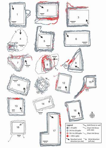
Figure 4b. (Continued)

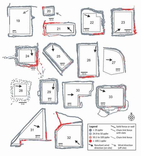
Concentration maps of facilities 12, 23, and 31 each reveal two distinct sections along the downwind perimeters with ΔCH₄ > 100 ppbv (Figure 4). Given relatively low wind direction variability at these facilities during the surveys (${\sigma }_{\theta }$ < 22.41°), we interpret these patterns as evidence of multiple emissions sources inside the perimeter. At select facilities (16 and 33), increases in CH₄ concentration occurred along sections of fence that were more porous, which correspond to gates for vehicle access.

The concentration map of facility 4 illustrates the effect of measurement distance on detection and attribution (Figure 4). Here a large (~0.1 m) diameter pipe is exposed above ground along the edge of a residential road. The main facility was located on the other side of the street but appears to have been decommissioned in recent years based on older photos from Google Street View. No enhancements >15 ppbv were detected while walking around the exposed pipe at a distance of several meters downwind. However, when we walked directly alongside the exposed pipe at close range (0.3 m), the peak ΔCH₄ was 952.6 ppbv, indicating the presence of a leak. This leak might not have been detected if direct access was prevented by a fence surrounding the pipe. This example – the only facility in the study without a fence – highlights a limitation of fence line measurements where equipment cannot be surveyed at close range.

Detection joint inference

At facilities with CH₃SH odor, peak ΔCH₄ ranged from 183.1 ppbv to 27865.3 ppbv, while at the other ten facilities the range was 3.2 ppbv to 198.8 ppbv (Table 1). Of the ten facilities without detected CH₃SH odor, three had peak ΔCH₄ mixing ratios >100 ppbv. For comparison, 100 ppbv is the upper limit of ΔCH₄ resolved by Chen et al. (2020) in a study of CH₄ emissions from a large festival in Germany. Facility rankings based on peak ΔCH₄ in Figure 5 indicate step changes between facilities ranked 3 and 4 (5741.7 ppbv to 1626.7 ppbv), 26 and 27 (119.1 ppbv to 48.8 ppbv), 30 and 31 (34.5 ppbv to 19.0 ppbv), and 32 and 33 (17.6 ppbv to 3.2 ppbv).

Figure 5. Facility rankings based on peak ΔCH_4.

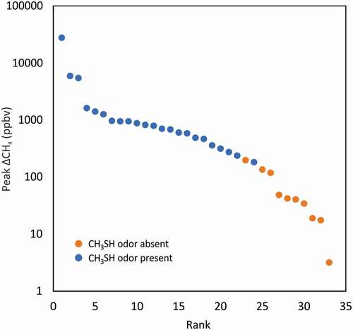
Results from our approach to differentiate upwind and downwind CH₄ enhancements show that the downwind ΔCH₄ 95^th percentiles are larger than upwind ΔCH₄ 95^th percentiles at 29/33 facilities (Table 1). The difference ranges from 36.1 ppbv to 8528.9 ppbv at all twenty-three facilities with detected CH₃SH odor, and from −26.5 ppbv to 48.6 ppbv at facilities without CH₃SH odor. Positive values suggest CH₄ emissions sources located inside the perimeter fence, whereas negative values suggest CH₄ emissions from other sources upwind.

Based on the emissions plausibility criteria, we interpret that twenty-two facilities had a high plausibility of emitting CH₄, followed by two with a medium plausibility, and eight with a low plausibility. In only one case are we certain that a leak was detected from above-ground pipe (facility 4).

Emissions quantification

Screening-level emissions fluxes and data quality indicators from six facilities interpreted as having a high plausibility of emissions are shown in Table 2. These facilities are ranked 2, 4, 5, 13, 14, and 15 in terms of peak ΔCH₄ (Figure 5). The highest rate was at facility 32 (30.79 mg CH₄ s⁻¹), located in an industrial park. The lowest emissions rate was at facility 13 (1.27 mg CH₄ s⁻¹), located in a recreation area and bounded on all sides by pathways within 20 m of the facility center. The sum of emissions rates for the six facilities quantified is 66.31 mg CH₄ s⁻¹, with 46.4% of the total emissions being attributable to facility 32. This is equivalent to 2.1 tonnes CH₄ if fluxes remained constant for one year or 176.4 tonnes CO₂e at a global warming potential of 84.

Table 2. OTM33A EQ summary of emissions rate estimates, mean wind speeds ($\bar{u}$), measurement distances, stability classes, and data quality indicator (DQI) scores. Reported stability classes are averages during survey times based on the standard deviation of the 2D wind direction and turbulent intensity. Stability classes range from 1–7 with higher numbers representing increasingly stable conditions

ID	Emissions rate (mg CH4 s^−1)	$\bar{u}$ (m/s)	Downwind distance (m)	Estimated Wind Stability Class	DQI
9	3.40	1.86	10	3	18
12–1	1.95	2.57	10	4	39
12–2	2.02	3.19	10	4	29
13	1.27	3.17	10	4	39
21	11.32	2.48	10	4	8
24	15.56	2.95	10	6	8
32	30.79	3.15	20	3	12

Data quality indicators (DQIs) in Table 2 qualify the accuracy of emissions rate estimates produced with OTM33A procedures. DQI scores and emissions rates are inversely related. The top four emissions rates, comprising 92.1% of the total estimated emissions, have the lowest DQI scores (8–18), which suggest higher accuracy. The highest DQI scores (29 and 39) correspond to facilities with estimated emissions rates that comprise 7.9% of the total estimated emissions. The combined emissions rate for the top four facilities is 61.07 mg CH₄ s⁻¹. These facilities have a total footprint of 4410 m² enclosed by fencing. Area provides a proxy for site potential to emit as larger sites generally contain more or larger equipment. From this, the average emissions rate per unit area is 13.85 μg CH₄ m² s⁻¹. If emissions rates from these four facilities remained constant over one year, the total emission would be 1926.58 kg CH₄ or 436.92 g CH₄ m² yr⁻¹.

Discussion and conclusions

Our fence line measurements indicate that 25/33 (76%) above-ground natural gas distribution facilities surveyed in the City of Calgary were either directly emitting CH₄ or had a medium to high likelihood of emitting CH₄ into the atmosphere. We confirmed one fugitive source at one location; emissions were identified directly adjacent to an exposed pipe. We suspect sources at the other 24 locations were a combination of fugitives and vented emissions. The latter may be associated with fuel gas driven pneumatics used to regulate gas pressure, which if present, are known by the natural gas company and may explain why there are walls up to 3 m tall around facilities at some locations. Solid walls and low-porosity fencing act as wind breaks to reduce CH₃SH odor reaching nearby residential, recreational, and commercial areas. However, we found that they are not 100% effective for odor control as CH₃SH odor was detected at fence line at twenty-three facilities, and from public spaces downwind of eight facilities. This has potential to be interpreted as a nuisance odor, especially for the facilities located within or close to residential areas and high-use recreation areas.

We demonstrate that multiple different sources of qualitative and quantitative information can be integrated to infer emissions detection plausibility in a complex environment that is not conducive to traditional top-down measurement methods like vehicle-based OTM33A. The methodology developed for this study bridges a resolution gap noted in previous studies regarding the lack of granularity in attributing and quantifying facility-level emissions in urban areas (Hopkins et al. 2016). Given limited road access around above-ground natural gas facilities in Calgary, we determined that source attribution and quantification required a different approach. Our methodology emulates source assessment modes outlined in OTM33A (Thoma and Squier 2014). The main advantage is improved accessibility, addressing the limitation vehicle-based systems have with road or facility access when measuring CH₄ across complex topographies and in urban areas. This enabled measurements at closer proximity to sources and the ability to acquire bounding-box measurements around facilities, reducing ambiguity in attributing emissions to sources inside the fence line. Further, grouping concentration measurements into upwind and downwind groups enabled more objective attribution of CH₄ emissions sources.

There are limitations of the methodology to consider for future applications involving attribution and quantification of facility-level CH₄ emissions in urban settings. First, the methodology is designed for measurements at a standoff distance dictated by fencing around the facility or other access restrictions. Attributing emissions to component-level sources from measurements at fence line is not possible with the methodology, nor can vents be distinguished from fugitives. However, the advantage is that facility-level measurements for emissions detection, attribution, and quantification can be acquired independently for research purposes without needing permission and coordination with the natural gas company to gain facility access for component-level surveys. One potential improvement to the sampling methodology is to attach a hose to the intake of the trace gas analyzer and elevate it above the fence using a light pole. Second, our application of OTM33A EQ diverges from previous applications in several ways. In this study, average distance to source was ~10 m compared to the recommended 20– 200 m. Furthermore, OTM33A has always been performed with a vehicle system and for much larger emission rates. Future work should evaluate backpack-based OTM33A EQ with controlled release testing. Third, the urban setting presents many challenges. The presence of near-field obstructions such as buildings, structures, and solid walls or low-porosity fencing modifies and deflects windflow within and around facilities, which affects plume mixing and dispersion. Research has shown that walls and other barriers create downwind concentration deficits due to upward deflection of wind flow and increased vertical mixing (Finn et al. 2010; Heist, Perry, and Brixey 2009). We suspect downwind CH₄ concentration deficits occurred at facilities where solid walls or low-porosity fencing was present, which could affect our assessment of emissions plausibility. Walls and low-porosity fencing also affect the reliability of emissions rate estimates, which limited our sample size.

Emissions fluxes from the sub-sample of natural gas facilities surveyed in Calgary are generally much lower than estimates from upstream oil and gas facilities for studies using OTM33A (Robertson et al. 2017). It is difficult to compare our flux estimates with other urban measurements and sources given different quantification approaches (e.g., Chen et al. 2020; Hendrick et al. 2016; Lamb et al. 2016, 2015, 1995; McKain et al. 2015; Plant et al. 2019) and the small sample size in our study. However, if the aggregate emissions rate from our OTM33A quantifications was converted to g CH₄ minute ⁻¹, results are comparable to the emissions factor obtained by Lamb et al. (2015) of 4.06 g CH₄ minute⁻¹ for M&R stations in the U.S. with gas pressures >300 psi. Overall, the emissions rates found at facilities where quantification was possible represent a small source of urban CH₄ emissions in comparison to other anthropogenic sources like landfills and waste treatment.

In the context of natural gas pricing at the time of the surveys (<3 CAD per GJ), the fluxes likely have negligible financial implications for the natural gas company as lost product. The costs associated with lost product, however, may be recovered by the utility provider through increased charges for customers. Losses from the natural gas distribution system can be mitigated by leak detection and repair (LDAR) and by converting emitting devices (e.g., pneumatics) to non-emitting devices that use compressed air, electricity, or hydraulics (International Energy Agency (IEA) 2020). Regardless of whether the sources are vents or fugitives, these emissions represent easy mitigation opportunities given the urban context and accessibility.

Acknowledgment

The authors acknowledge equipment support from the University of Calgary Global Research Initiative.

Disclosure statement

No potential conflict of interest was reported by the author(s).

Additional information

Notes on contributors

Chris H. Hugenholtz

Chris H. Hugenholtz is a Professor Parex Innovation Fellow, and Director of the Centre for Smart Emissions Sensing Technologies, University of Calgary.

Coleman Vollrath

Coleman Vollrath is an MSc student and Research Assistant.

Tyler Gough

Tyler Gough is a PhD student and Research Assistant.

Clay Wearmouth

Clay Wearmouth is an MSc student and Research Technician.

Thomas Fox

Thomas Fox is a President and Director of Innovation, Highwood Emissions Management.

Thomas Barchyn

Thomas Barchyn is a Research Project Manager.

Chandler Billinghurst

Chandler Billinghurst is an MSc student.

References

- Alvarez, R. A., D. Zavala-Araiza, D. R. Lyon, D. T. Allen, Z. R. Barkley, A. R. Brandt, K. J. Davis, S. C. Herndon, D. J. Jacob, A. Karion, et al. 2018. Assessment of methane emissions from the US oil and gas supply chain. Science 361 (6398):186–88. doi:https://doi.org/10.1126/science.aar7204.
- Alvarez, R. A., S. W. Pacala, J. J. Winebrake, W. L. Chameides, and S. P. Hamburg. 2012. Greater focus needed on methane leakage from natural gas infrastructure. Proc. Natl. Acad. Sci. 109 (17):6435–40. doi:https://doi.org/10.1073/pnas.1202407109.
- Brantley, H. L., E. D. Thoma, W. C. Squier, B. B. Guven, and D. R. Lyon. 2014. Assessment of methane emissions from oil and gas production pads using mobile measurements. Environ. Sci. Technol. 48 (24):14508–15. doi:https://doi.org/10.1021/es503070q.
- Chen, J., F. Dietrich, H. Maazallahi, A. Forstmaier, D. Winkler, M. E. G. Hofmann, H. D. van der Gon, and T. Röckmann. 2020. Methane emissions from the Munich Oktoberfest. Atmospheric Chem. Phys. 20 (6):3683–96. doi:https://doi.org/10.5194/acp-20-3683-2020.
- Edie, R., A. M. Robertson, R. A. Field, J. Soltis, D. A. Snare, D. Zimmerle, C. S. Bell, T. L. Vaughn, and S. M. Murphy. 2020. Constraining the accuracy of flux estimates using OTM 33A. Atmos. Meas. Tech. 13 (1):341–53. doi:https://doi.org/10.5194/amt-13-341-2020.
- Finn, D., K. L. Clawson, R. G. Carter, J. D. Rich, R. M. Eckman, S. G. Perry, V. Isakov, and D. K. Heist. 2010. Tracer studies to characterize the effects of roadside noise barriers on near-road pollutant dispersion under varying atmospheric stability conditions. Atmos. Environ. 44 (2):204–14. doi:https://doi.org/10.1016/j.atmosenv.2009.10.012.
- Heist, D. K., S. G. Perry, and L. A. Brixey. 2009. A wind tunnel study of the effect of roadway configurations on the dispersion of traffic-related pollution. Atmos. Environ. 43 (32):5101–11. doi:https://doi.org/10.1016/j.atmosenv.2009.06.034.
- Heltzel, R. S., M. T. Zaki, A. K. Gebreslase, O. I. Abdul-Aziz, and D. R. Johnson. 2020. Continuous OTM 33A analysis of controlled releases of methane with various time periods, data rates and wind filters. Environments 7 (9):65. doi:https://doi.org/10.3390/environments7090065.
- Hendrick, M. F., R. Ackley, B. Sanaie-Movahed, X. Tang, and N. G. Phillips. 2016. Fugitive methane emissions from leak-prone natural gas distribution infrastructure in urban environments. Environ. Pollut. 213:710–16. doi:https://doi.org/10.1016/j.envpol.2016.01.094.
- Hopkins, F. M., J. R. Ehleringer, S. E. Bush, R. M. Duren, C. E. Miller, C.-T. Lai, Y.-K. Hsu, V. Carranza, and J. T. Randerson. 2016. Mitigation of methane emissions in cities: How new measurements and partnerships can contribute to emissions reduction strategies. Earth’s Future 4 (9):408–25. doi:https://doi.org/10.1002/2016EF000381.
- Howarth, R. W. 2014. A bridge to nowhere: Methane emissions and the greenhouse gas footprint of natural gas. Energy Sci. Eng. 2 (2):47–60. doi:https://doi.org/10.1002/ese3.35.
- International Energy Agency (IEA). 2020. Methane tracker 2020. Accessed October5, 2020. https://www.iea.org/reports/methane-tracker-2020.
- Jackson, R. B., A. Down, N. G. Phillips, R. C. Ackley, C. W. Cook, D. L. Plata, and K. Zhao. 2014. Natural gas pipeline leaks across Washington, DC. Environ. Sci. Technol. 48 (3):2051–58. doi:https://doi.org/10.1021/es404474x.
- Klausner, T., M. Mertens, H. Huntrieser, M. Galkowski, G. Kuhimann, R. Baumann, A. Fiehn, P. Jöckel, M. Pühl, and A. Roiger. 2020. Urban greenhouse gas emissions from the Berlin area: A case study using airborne CO2 and CH4 in situ observations in summer 2018. Elementa 8:15. doi:https://doi.org/10.1525/elementa.411.
- Lamb, B. K., J. B. McManus, J. H. Shorter, C. E. Kolb, B. Mosher, R. C. Harriss, E. Allwine, D. Blaha, T. Howard, A. Guenther, et al. 1995. Development of atmospheric tracer methods to measure methane emissions from natural gas facilities and urban area. Environ. Sci. Technol. 29 (6):1468–79. doi:https://doi.org/10.1021/es00006a007.
- Lamb, B. K., M. O. L. Cambaliza, K. J. Davis, S. L. Edburg, T. W. Ferrara, C. Floerchinger, A. M. F. Heimburger, S. Herndon, T. Lauvaix, T. Lavoie, et al. 2016. Direct and indirect measurements and modeling of methane emissions in Indianapolis, Indiana. Environ. Sci. Technol. 50 (16):8910–17. doi:https://doi.org/10.1021/acs.est.6b01198.
- Lamb, B. K., S. L. Edburg, T. W. Ferrara, T. Howard, M. R. Harrison, C. E. Kolb, A. Townsend-Small, W. Dyck, A. Possolo, and J. R. Whetstone. 2015. Direct measurements show decreasing methane emissions from natural gas local distribution systems in the United States. Environ. Sci. Technol. 49 (8):5161–69. doi:https://doi.org/10.1021/es505116p.
- McKain, K., A. Down, S. M. Raciti, J. Budney, L. R. Hutyra, C. Floerchinger, S. C. Herndon, T. Nehrkorn, M. S. Zahniser, R. B. Jackson, et al. 2015. Methane emissions from natural gas infrastructure and use in the urban region of Boston, Massachusetts. Proc. Natl. Acad. Sci. 112 (7):1941–46. doi:https://doi.org/10.1073/pnas.1416261112.
- Myhre, G., D. Shindell, F.-M. Bréon, W. Collins, J. Fuglestvedt, J. Huang, D. Koch, J.-F. Lamarque, D. Lee, B. Mendoza, et al. 2013. Anthropogenic and natural radiative forcing. In Climate change 2013: The physical science basis. contribution of working Group I to the fifth assessment report of the intergovernmental panel on climate change, ed. T. F. Stocker, D. Qin, G.-K. Plattner, M. Tignor, S. K. Allen, J. Boschung, A. Nauels, Y. Xia, V. Bex, and P. M. Midgley, 714. Cambridge, UK; New York, USA: Cambridge University Press.
- Phillips, N. G., R. Ackley, E. R. Crosson, A. Down, L. R. Hutyra, M. Brondfield, J. D. Karr, K. Zhao, and R. B. Jackson. 2013. Mapping urban pipeline leaks: Methane leaks across Boston. Environ. Pollut. 173:1–4. doi:https://doi.org/10.1016/j.envpol.2012.11.003.
- Pierrehumbert, R. T. 2014. Short-lived climate pollutants. Annu. Rev. Earth Planet. Sci. 42 (1):341–79. doi:https://doi.org/10.1146/annurev-earth-060313-054843.
- Plant, G., E. A. Kort, C. Floerchinger, A. Gvakharia, I. Vimont, and C. Sweeney. 2019. Large fugitive methane emissions from urban centers along the US East Coast. Geophys. Res. Lett. 46 (14):8500–07. doi:https://doi.org/10.1029/2019GL082635.
- Ren, X., O. E. Salmon, J. R. Hansford, D. Ahn, D. Hall, S. E. Benish, P. R. Stratton, H. He, S. Sahu, C. Grimes, et al. 2018. Methane emissions from the Baltimore-Washington area based on airborne observations: Comparison to emissions inventories. J. Geophys. Res. 123:8869–82. doi:https://doi.org/10.1029/2018JD028851.
- Robertson, A. M., R. Edie, D. Snare, J. Soltis, R. A. Field, M. D. Burkhart, and S. M. Murphy. 2017. Variation in methane emission rates from well pads in four oil and gas basins with contrasting production volumes and compositions. Environ. Sci. Technol. 51 (15):8832–40. doi:https://doi.org/10.1021/acs.est.7b00571.
- Sanchez, N. P., C. Zheng, W. Ye, B. Czader, D. S. Cohan, F. K. Tittel, and C. H. Griffin. 2018. Exploratory study of atmospheric methane enhancement derived from natural gas use in the Houston urban area. Atmos. Environ. 176:261–73. doi:https://doi.org/10.1016/j.atmosenv.2018.01.001.
- Thoma, E., and B. Squier. 2014. OTM 33 Geospatial Measurement of Air Pollution, Remote Emissions Quantification (GMAP-REQ) and OTM33A Geospatial Measurement of Air Pollution-Remote Emissions Quantification-Direct Assessment (GMAP-REQ-DA). Cincinnati, OH: US Environmental Protection Agency.
- von Fischer, J. C., D. Cooley, S. Chamberlain, A. Gaylord, C. J. Griebenow, S. P. Hamburg, J. Salo, R. Schumacher, D. Theobald, and J. Ham. 2017. Rapid, vehicle-based identification of location and magnitude of urban natural gas pipeline leaks. Environ. Sci. Technol. 51 (7):4091–99. doi:https://doi.org/10.1021/acs.est.6b06095.
- Weller, Z., S. P. Hamburg, and J. C. von Fischer. 2020. A national estimate of methane leakage from pipeline mains in natural gas local distribution systems. Environ. Sci. Technol. 54 (14):8958–67. doi:https://doi.org/10.1021/acs.est.0c00437.
- Wunch, D., G. C. Toon, J. K. Hedelius, N. Vizenor, C. M. Roehl, K. M. Saad, J.-F. L. Blavier, D. R. Blake, and P. O. Wennberg. 2016. Quantifying the loss of processed natural gas within California’s South Coast Air Basin using long-term measurements of ethane and methane. Atmospheric Chem. Phys. 16 (22):14091–105. doi:https://doi.org/10.5194/acp-16-14091-2016.
- Yamartino, R. J. 1984. A comparison of several “single-pass” estimators of the standard deviation of wind direction. Journal of Applied Meteorology and Climatology. 23(9):1362–66.