Regional temperature-ozone relationships across the U.S. under multiple climate and emissions scenarios

ABSTRACT

The potential effects of 21st century climate change on ozone (O₃) concentrations in the United States are investigated using global climate simulations to drive higher-resolution regional meteorological and chemical transport models. Community Earth System Model (CESM) and Coupled Model version 3 (CM3) simulations of the Representative Concentration Pathway 8.5 scenario are dynamically downscaled using the Weather Research and Forecasting model, and the resulting meteorological fields are used to drive the Community Multiscale Air Quality model. Air quality is modeled for five 11-year periods using both a 2011 air pollutant emission inventory and a future projection accounting for full implementation of promulgated regulatory controls. Across the U.S., CESM projects daily maximum temperatures during summer to increase 1–4°C by 2050 and 2–7°C by 2095, while CM3 projects warming of 2–7°C by 2050 and 4–11°C by 2095. The meteorological changes have geographically varying impacts on O₃ concentrations. Using the 2011 emissions dataset, O₃ increases 1–5 ppb in the central Great Plains and Midwest by 2050 and more than 10 ppb by 2095, but it remains unchanged or even decreases in the Gulf Coast, Maine, and parts of the Southwest. Using the projected emissions, modeled increases are attenuated while decreases are amplified, indicating that planned air pollution control measures ameliorate the ozone climate penalty. The relationships between changes in maximum temperature and changes in O₃ concentrations are examined spatially and quantified to explore the potential for developing an efficient approach for estimating air quality impacts of other future climate scenarios.

Implications: The effects of climate change on ozone air quality in the United States are investigated using two global climate model simulations of a high warming scenario for five decadal periods in the 21st century. Warming summer temperatures simulated under both models lead to higher ozone concentrations in some regions, with the magnitude of the change increasing with temperature over the century. The magnitude and spatial extent of the increases are attenuated under a future emissions projection that accounts for regulatory controls. Regional linear regression relationships are developed as a first step toward development of a reduced form model for efficient estimation of the health impacts attributable to changes in air quality resulting from a climate change scenario.

Introduction

Ozone (O₃) is an air pollutant formed in the troposphere from photochemical reactions between nitrogen oxides (NO_x) and volatile organic compounds (VOCs), which are emitted from various natural and anthropogenic sources. Ozone mixing ratios are strongly influenced by the absolute and relative abundances of NO_x and VOCs, as well as meteorological parameters including temperature, wind speeds, mixing depths, humidity, clouds, and precipitation. Changes in the means or distributions of any of these meteorological quantities could potentially affect concentrations of ozone and other air pollutants. Numerous studies that have used global or regional chemical transport models forced by future global climate model (GCM) data have concluded that for a given level of anthropogenic emissions of precursors, climate change increases surface O₃ concentrations in some polluted continental regions (Fiore, Naik, and Leibensperger 2015; Fiore et al. 2012; Fu and Tian 2019; Jacob and Winner 2009; Nolte et al. 2008). This “climate penalty” (Wu et al. 2008) has been attributed principally to warmer temperatures increasing NO_x via thermal decomposition of peroxyacetyl nitrates and increasing emissions of biogenic VOCs (Dawson, Adams, and Pandis 2007; Nolte et al. 2018; Weaver et al. 2009). Additionally, some studies have linked changing ozone air pollution in the U.S. to altered atmospheric circulation patterns, including frequency of frontal passages (Lee and Sheridan 2018; Leibensperger, Mickley, and Jacob 2008), shifts in the jet stream (Barnes and Fiore 2013) and storm tracks (Tamarin-Brodsky and Kaspi 2017), higher levels of stagnation (Leung and Gustafson 2005). and increased frequency and intensity of heat waves (Gao et al. 2013).

Higher peak ozone levels could render some areas out of compliance with the U.S. National Ambient Air Quality Standards, potentially requiring more stringent emissions controls (Avise et al. 2012; Wu et al. 2008). Degraded air quality due to climate change would also have important implications for public health and welfare, including increased risks of premature mortality, aggravated asthma, and other respiratory or cardiovascular conditions requiring admission to hospital emergency departments. In multisector analyses of the impacts of climate change in the United States, air quality damages are among the largest economic impacts (EPA 2015a; Martinich and Crimmins 2019). Prior studies have suggested that changes in air quality due to climate change could result in tens to thousands of premature deaths, hospital admissions, and cases of acute respiratory illnesses in the United States annually, with economic damages estimated in the hundreds of millions to tens of billions of U.S. dollars (Bell et al. 2007; Fann et al. 2015, 2021; Garcia-Menendez et al. 2015; Martinich and Crimmins 2019; Post et al. 2012).

To further explore the impacts of future climate scenarios on air quality, in this work a regional chemical transport model is driven by meteorology that was dynamically downscaled from two global climate model simulations over the conterminous U.S. for multiple periods in the 21st century. Simulations are conducted using both a recent air pollutant emissions inventory and a future projection accounting for the implementation of promulgated regulatory actions to control emissions. We examine the climate change impacts on ozone air quality due to changing meteorology and how those impacts vary under the two anthropogenic air pollutant emissions datasets. The analysis is focused on changes in seasonal means of daily maximum 8-h average (MDA8) ozone values, motivated by health impacts calculated using this metric (EPA 2015b; Fann et al. 2021).

Air quality impacts have not been considered in most U.S. policy analyses of the economic impacts of future climate scenarios, largely due to the high computational expense of creating long-term simulations of atmospheric chemistry and lack of availability of the comprehensive suite of meteorological fields required to drive those simulations. Consequently, those multisector analyses that have included air quality (EPA 2015a, 2017) have considered a limited number of climate scenarios. A reduced form approach, if available and credible, would increase the capacity to consider air quality and health impacts in multisector assessments across a broader range of future scenarios. While there are many meteorological factors that influence ozone concentrations, temperature has been shown repeatedly to be the strongest determinant (Camalier, Cox, and Dolwick 2007; Dawson, Adams, and Pandis 2007; Jacob et al. 1993; Porter et al. 2015; Rasmussen et al. 2012; Sillman and Samson 1995; Wells et al. 2021). As a step toward possible development of a reduced form model to efficiently estimate the health impacts attributable to changes in air quality resulting from a given climate change scenario, the relationships between simulated changes in temperatures and ozone concentrations are explored for different regions of the U.S. under the two climate scenarios and two air pollutant emission scenarios.

Methods

Global climate modeling

This study uses simulations from the National Center for Atmospheric Research-Department of Energy Community Earth System Model version 1 (CESM; Gent et al. 2011) and the Geophysical Fluid Dynamics Laboratory Coupled Model version 3 (CM3; Donner et al. 2011) that were conducted for the fifth phase of the Coupled Model Intercomparison Project (CMIP5; Taylor, Stouffer, and Meehl 2012). The last 11 years of the historical 20th century experiment (i.e., 1995–2005) and the period 2025–2100 following Representative Concentration Pathway 8.5 (RCP8.5) were selected for dynamical downscaling. The RCP8.5 scenario (Riahi et al. 2011) assumes high growth in population, energy demand, and emissions of greenhouse gases (GHGs), resulting in 8.5 W m⁻² of radiative forcing at 2100 (relative to preindustrial conditions), and mean temperature increases over the conterminous U.S. of 3.2–6.6°C relative to 1976–2005 (Vose et al. 2017). Due to computational constraints, downscaled meteorology from only one GHG concentration scenario was used to model air quality. RCP8.5 was chosen to facilitate analysis of the broadest range of temperature changes. Of the four RCP scenarios, RCP8.5 aligns best with historical cumulative CO₂ emissions and projections out to 2050 under current and stated policies (Schwalm, Glendon, and Duffy 2020). Research is ongoing as to the likelihood of the high levels of GHG emissions in RCP8.5 after 2050 in the absence of a global climate policy (Burgess et al. 2020; Christensen, Gillingham, and Nordhaus 2018; Hausfather and Peters 2020; Schwalm, Glendon, and Duffy 2020).

Regional climate modeling

Archived 6-h fields from the CESM and CM3 simulations conducted for CMIP5 were dynamically downscaled to a 36 × 36 km North American domain (Figure 1) using the Weather Research and Forecasting (WRF) model (Skamarock and Klemp 2008). The approximately 1° latitude × 1° longitude CESM fields were downscaled directly using WRF version 3.4.1 with modifications to the Kain-Fritsch cumulus parameterization to include radiative feedbacks (Herwehe et al. 2014); these modifications were publicly released in WRF version 3.6. The 2° × 2.5° CM3 fields were downscaled with WRF version 3.6 using two-way, 108- and 36-km nested domains, where the 36-km domain was the same as for CESM. Both WRF simulations were performed using 34 vertical layers extending to 50 hPa. WRF was initialized on 1 October 1994 for the historical runs and 1 October 2024 for RCP8.5, providing a 3-month spin-up period for each, then run continuously without reinitialization for 1995–2005 and 2025–2100, respectively. Following our previous work (Bowden et al. 2012; Otte et al. 2012; Spero et al. 2016), all WRF simulations employed spectral nudging toward the driving GCM fields, and the chosen physics parameterizations follow those of Spero et al. (2016). To avoid the effects of spurious discontinuities that arise from using only ocean points to set water temperatures that are not resolved by the GCMs (Mallard et al. 2015), lake temperatures modeled by the Community Land Model (CLM, the land component of CESM) were used when downscaling CESM (Spero et al. 2016), while WRF was coupled to the FLake model when downscaling CM3 (Mallard et al. 2014).

Figure 1. WRF and CMAQ modeling domains at 36-km grid spacing. The WRF domain has 199 × 127 grid points, while the CMAQ domain is a subset comprised of 148 × 110 grid cells. Numbered areas represent the regions used for evaluation following the U.S. Fourth National Climate Assessment (USGCRP 2018): (1) Northwest; (2) Southwest; (3) Northern Great Plains; (4) Southern Great Plains; (5) Midwest; (6) Northeast; and (7) Southeast

Chemical transport modeling

The air quality simulations were conducted using a prerelease version of the Community Multiscale Air Quality (CMAQ) model version 5.3 (https://www.epa.gov/cmaq, last access: 19 July 2021) (Appel et al. 2021), with accommodations for the USGS28 (US Geological Survey 28-category, including lakes) land use scheme used in the WRF simulations. The model was configured with the CB6 chemical mechanism (Luecken, Yarwood, and Hutzell 2019), the AERO7 aerosol module, and the Surface Tiled Aerosol and Gaseous Exchange (STAGE) dry deposition option (Appel et al. 2021). CMAQ simulations were conducted over a 36-km domain covering the conterminous U.S. (Figure 1). The Meteorology-Chemistry Interface Processor (MCIP; Otte and Pleim 2010) version 4.5.1 was used to create meteorological inputs for CMAQ using the same vertical layer structure as in WRF.

CMAQ was run for five 11-year periods, centered on 2000, 2030, 2050, 2075, and 2095, using WRF meteorology downscaled from both CESM and CM3. CMAQ was initialized on 21 December to provide a 10-day spin-up period prior to each 11-year continuous simulation. For each scenario and period, CMAQ simulations were conducted using two anthropogenic emissions datasets, resulting in 220 annual simulations. Both emissions datasets were based on the 2011 National Emissions Inventory (NEI): a 2011 base case and the 2040 reference case projection used in the analysis of the heavy-duty vehicle greenhouse gas rule (EPA 2016). Projected emissions in 2040 were substantially lower than for 2011 (Table 1) because the projection assumed the implementation of promulgated regulatory measures, including the Cross-State Air Pollution Rule, the Mercury and Air Toxics rule, and Tier 3 motor vehicle emission and fuel standards.

Table 1. Annual total anthropogenic emissions in conterminous U.S. (Tg yr⁻¹) used in CMAQ simulations

Species	2011	2040	Difference (%)
CO	64.8	46.5	−28.2
NOx	12.9	6.3	−51.1
VOC	15.7	13.5	−14.1
SO2	5.8	2.0	−65.8
NH3	3.8	3.9	2.0
PM2.5	4.2	4.1	−2.5

Biogenic emissions were modeled within CMAQ using the Biogenic Emission Inventory System (BEIS) version 3.61 (Bash, Baker, and Beaver 2016) with the downscaled meteorology. Chemical lateral boundary conditions derived from a simulation of the year 2011 by the GEOS-Chem global chemical transport model (Henderson et al. 2014) were used for each of the annual simulations. No assumptions were made within CMAQ related to changes in background concentrations of carbon dioxide, methane, or other atmospheric constituents, or to changes in land use, land cover, or the geographic distribution of different species of vegetation and their associated biogenic emissions, or to emissions from wildfires. Finally, the atmospheric formation of NO from lightning was not modeled.

We acknowledge that the 36-km grid spacing used here is insufficient to represent the meteorological flow near coastlines and in areas of complex terrain, and the strong spatial gradients in emissions within urban areas. However, it is impractical to adopt finer horizontal grid spacing (typically employed for annual or shorter modeling periods) for multi-decadal climate and air quality simulations across the U.S. The present manuscript focuses on differences in multiyear seasonal means, motivated by health effects calculations based on long-term average concentrations. While air pollutant concentrations simulated using 36-km and 12-km model configurations exhibit episodic differences, the differences in long-term trends are small (Gan et al. 2016). Differences in extreme values of temperature and ozone are likely to be accentuated by using finer horizontal grid spacing. Nevertheless, the 36-km grid spacing used here is sufficient to assess the broad regional interpretation of the temperature-ozone relationship.

Results

Representation of baseline conditions

Temperature

Daily maximum temperature is the focus of the meteorological evaluation because of its strong influence on photochemistry and ozone formation (Camalier, Cox, and Dolwick 2007; Porter et al. 2015; Rasmussen et al. 2012; Wells et al. 2021). The global Climate Forecast System Reanalysis (CFSR; Saha et al. 2010) archives hourly temperature at 0.31° resolution and is therefore suitable for evaluation of modeled daily maximum temperatures. CFSR fields for 1995–2005 are interpolated to the 36-km WRF grid for comparison. Analysis is performed using region definitions (Figure 1) from the U.S. Fourth National Climate Assessment (NCA4; USGCRP 2018). Seasonal averages of daily maximum temperatures simulated when downscaling CESM are generally well represented (Supplemental Figure 1b), though biases exceeding 4°C occur in the intermountain west and the Pacific coast where the complex terrain is not well resolved at 36-km horizontal grid spacing. Regionally averaged absolute biases in daily maximum temperatures are 1.1°C or less during summer and are less than 2°C for most regions and seasons (Supplemental Table 1). Maximum temperatures in the Northeast are positively biased by 3.2°C in the spring and 2.2°C in the fall, while during the spring a positive bias of 2.9°C exists in the Midwest and a negative bias of −2.4°C is simulated in the Southwest. When downscaling CM3 (Supplemental Figure 1d), daily maximum temperatures are negatively biased throughout the year over most of the conterminous U.S. The cool bias exceeds 4.0°C in the Northwest, Southwest, and Northern Great Plains during summer and in the Southwest and Southern Great Plains during spring. These biases in WRF emulate the biases in the global climate models (Supplemental Figure 1a, c), as we did not apply any bias correction prior to downscaling and we used spectral nudging to constrain WRF toward the CESM and CM3 fields (Bowden et al. 2012; Nolte et al. 2018; Otte et al. 2012).

Ozone

Summer (JJA) mean MDA8 ozone concentrations simulated using year 2011 emissions with the downscaled meteorology for 1995–2005 are evaluated by comparing to observations from the Air Quality System (AQS) and Clean Air Status and Trends Network (CASTNET) for the year 2011. AQS sites are primarily in urban and suburban locations, while CASTNET sites are rural. Daily values are computed for sites having a minimum of 16 hourly measurements, and sites with valid data for fewer than 75% of summer days are excluded. Sites with corresponding grid cell centers outside the U.S. or represented as water points in CMAQ are also excluded from the analysis. MDA8 ozone levels simulated using meteorology downscaled from CESM and CM3 compare reasonably well with observations (Figure 2), within 5 ppb for about half of the sites (45–61%) and within 10 ppb for 79–88% of sites. Positive biases exceeding 10 ppb occur in the Northeast and along the Gulf Coast using meteorology downscaled from both climate models and in the Midwest when using meteorology downscaled from CESM (Supplemental Figure 2). Negative biases exceeding 5 ppb exist at several sites in the Southwest, particularly in California. Regional average biases at AQS sites range from −1.3 to 8.9 ppb with CESM and −2.9 to 6.1 under CM3 (Table 2), with mean biases across all 1127 sites of 4.1 and 1.6 ppb, respectively. Simulated O₃ is generally lower throughout the conterminous U.S. using meteorology from CM3 compared to CESM due to the overall cooler temperatures in CM3 during this modeled period (Supplemental Figure 1). These biases in O₃ simulated using downscaled climate model data are comparable in magnitude to the median biases of 10 ppb obtained by Seltzer et al. (2016) using reanalysis (i.e., true historical) meteorology.

Table 2. Regionally averaged biases (ppb) in modeled^a summer season MDA8 O₃ compared to year 2011 observations at AQS and CASTNET sites

	AQS			CASTNET
Region	n^b	CESM	CM3	n	CESM	CM3
Northwest	27	4.3	1.8	1	12.4	9.6
Southwest	307	−1.3	−2.9	15	−6.0	−7.9
Northern Great Plains	36	2.3	−1.5	7	−2.3	−5.0
Southern Great Plains	92	2.8	1.6	5	1.7	−2.2
Midwest	224	8.0	2.9	14	3.5	−0.2
Southeast	266	4.5	3.1	20	4.4	2.6
Northeast	175	8.9	6.1	15	6.9	5.3
All Regions	1127	4.1	1.6	77	2.0	−0.3

^aCMAQ modeling results using 2011 emissions and all 11 years of the baseline 1995–2005 periods downscaled from CESM and CM3. ^b Number of sites; see Supplemental Figure 2 for maps.

Figure 2. Histograms of bias (ppb) in summer average daily maximum 8-h O₃ compared to 2011 observations at AQS (a, b) and CASTNET (c, d) sites using meteorology downscaled from CESM (a, c) and CM3 (b, d)

Temperature-ozone relationships

The relationships between co-located observations of daily maximum temperatures and MDA8 O₃ at CASTNET sites are compared to those simulated using downscaled meteorology for 1995–2005 and 2011 emissions (Figure 3). Three summers of CASTNET observations (2010–2012) are used to increase the statistical power of the analysis. The CASTNET observations demonstrate a strong positive relationship between observed temperature and ozone exists in the Northwest, Midwest, and Northeast regions, with slopes (m) ranging from 1.36 to 2.09 ppb °C⁻¹ and coefficients of determination (R²) values of 0.41–0.47. The association is suggestive but weaker in the Southern Great Plains and Southwest, with slopes of 1.19 and 0.56 ppb °C⁻¹ but much lower values of R². By contrast, there is no significant relationship between temperature and ozone at CASTNET sites in the Northern Great Plains and the Southeast, with R² values near 0. The spatial and temporal variability of the temperature-ozone relationship is, in part, attributable to differences in chemical and meteorological processes affecting O₃ formation, particularly the NO_x to VOC ratio and whether the location is in the NO_x-sensitive or VOC-sensitive regime (Fu and Tian 2019; Pusede and Cohen 2012; Rasmussen et al. 2013; Steiner et al. 2010).

Figure 3. Observed and CMAQ-modeled relationships between daily maximum 8-h O₃ and daily maximum temperature from 1 June – 31 August with slopes m (ppb °C⁻¹) and R² of best-line fits. Observations are from 77 CASTNET sites during 2010–2012; modeled results use meteorology downscaled from CESM and CM3 for 1995–2005 and year 2011 emissions. Region definitions are provided in Figure 1

The modeled relationships between ozone and temperature are in generally good agreement with the CASTNET data. Using meteorology downscaled from both CESM and CM3, the modeled ozone-temperature relationship is strongly positive in the Northwest, Midwest, and Northeast regions, with slopes within 20–30% of those in the CASTNET data. Likewise, the modeling shows no significant relationship between temperature and ozone in the Southeast. Results for the Southwest and Northern and Southern Great Plains regions are mixed, with the CESM simulation showing a weak but positive relationship while the CM3 run has slopes and R² close to 0.

Changes over the 21^st century

Temperature

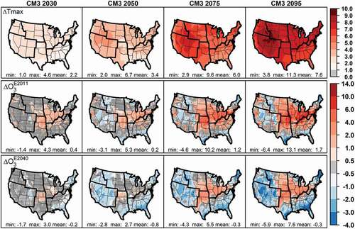
Temperatures simulated by downscaling both climate models generally increase over time, with some interannual variability. Daily maximum temperatures averaged over the May–September ozone season and over the NCA4 regions increase 0.41–0.55°C decade⁻¹ when downscaling CESM and 0.69–0.88°C decade⁻¹ when downscaling CM3 (Supplemental Figure 3). At 2050, daily maximum temperatures (Figure 4) increase by ≥1.0°C everywhere in the conterminous U.S. with CESM and by ≥2.0°C with CM3 (Figure 5). At 2095, May–September daily maximum temperatures simulated when downscaling CESM are 2.3–7.0°C higher than at 2000, while increases under CM3 range from 2.8–11.3°C and exceed 8°C over much of the western U.S. Despite the higher rate of warming, absolute temperatures obtained when downscaling CM3 to 2100 remain slightly lower than with CESM in most regions, due to the cool bias in CM3 at 2000 (Supplemental Figure 3). All simulated increases in daily maximum temperature shown are statistically significant, except for a few points at 2030 under CESM.

Figure 4. Changes relative to 2000 using meteorology downscaled from CESM. Top row: daily maximum temperatures (°C). Bottom two rows: MDA8 O₃ (ppb) using emissions from 2011 and 2040, respectively. All quantities shown are differences in May–September averages between the 11-year period centered on the indicated year and the downscaled representation of 1995–2005. Stippling indicates differences are not statistically significant at the p = .05 level

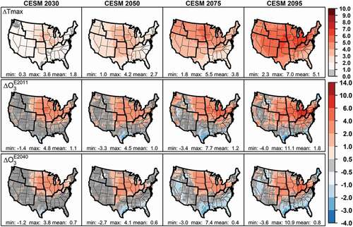
Figure 5. As in Figure 4, but using meteorology downscaled from CM3

Ozone

Climate change, as reflected in the downscaled meteorology, alters modeled ozone air quality. Relative to 2000, MDA8 O₃ concentrations simulated using 2011 emissions and meteorology downscaled from CESM increase by 0.5–4.8 ppb throughout most of the eastern U.S. at 2030 (Figure 4). Ozone increases throughout the century, such that at 2095 concentrations are ≥6 ppb higher in parts of the Midwest, and the area with increased concentrations includes much of the Northwest and Southwest. The magnitude and spatial extent of the increases in MDA8 O₃ are generally slightly smaller using meteorology downscaled from CM3 (Figure 5), despite the greater response in temperature. Both models project maximum increases occurring in the Northern Great Plains and Midwest and parts of the Northeast and Northwest regions, with comparatively little change in most of the Southeast and Southwest regions. Both models show O₃ decreases in Maine, southern Texas, and along the Gulf Coast that intensify over time, while CM3 additionally projects decreases in much of the Southwest outside California. These decreases are likely attributable to increased biogenic VOC emissions in regions which are already NO_x-limited, causing a decrease in O₃ production efficiency, or even providing additional OH radicals that act as an O₃ sink (Porter and Heald 2019; Weaver et al. 2009).

Changes for selected percentiles of the MDA8 O₃ distribution are provided in Supplemental Figure 4. Using meteorology downscaled from CESM under multiple RCPs at 2030, Nolte et al. (2018) reported greater increases at upper percentiles in the eastern U.S. Consistent with Nolte et al. (2018), here we find increases are highest at the upper end of the distribution for most regions at 2050 and 2095 under both climate scenarios. The increases are strongest in the Northeast, Midwest, and Southeast, with 98th percentile increases reaching 2–4 ppb at 2050 and 5–8 ppb at 2095 relative to the historical periods.

As expected, the magnitude and areal extent of ozone increases are attenuated using 2040 emissions, particularly later in the century, due to the decreased emissions of NO_x in that projection. This analysis indicates that the planned reductions in the future emissions projection decrease the impact of the climate penalty for ozone. Interestingly, the decreases projected in Maine, Texas, the Southeast, and Nevada are amplified using 2040 emissions. This is especially true for CM3 at 2095, which indicates decreases exceeding 3 ppb over much of the country.

Relationships between changes in temperature and O₃

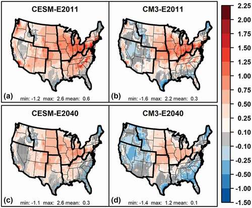
Anomalies of May–September mean MDA8 O₃ and daily maximum temperature were computed for each future year relative to the 1995–2005 baseline. Linear models were constructed relating ozone and temperature anomalies so that the resulting regression coefficients estimate the climate penalty (ppb increase in MDA8 O₃ per degree Celsius increase in temperature) at each grid cell (Figure 6). Using meteorology downscaled from CESM with 2011 emissions, values range from 0.5–1.75 ppb °C⁻¹ over most of the Northern Great Plains, Midwest, and Northeast and parts of the Northwest, Southwest, and Southeast regions (Figure 6a). Climate penalties obtained using meteorology downscaled from CM3 with 2011 emissions (Figure 6b) are similar in magnitude to CESM but are more localized to the central and Midwest regions of the country. Consistent with the ozone decreases in Figures 4 and 5, negative slopes (i.e., decreases in O₃ with increasing temperatures) are obtained in Maine, the Gulf Coast, and parts of the Southwest. The negative relationship between temperature and O₃ in Texas and the Southeast has been reported previously (Camalier, Cox, and Dolwick 2007; Porter et al. 2015; Shen, Mickley, and Gilleland 2016) and is statistically significant (p < .05) under CM3, but not under CESM. Even though these negative slopes under CM3 are statistically significant, the very low values of R² (Supplemental Figure 5) indicate that other factors besides temperature account for a greater portion of the variability in O₃ in those areas. Regression coefficients calculated using projected 2040 emissions (Figure 6c–d) are lower than those calculated using 2011 emissions, consistent with prior literature concluding that the climate penalty diminishes with decreasing levels of NO_x emissions (Bloomer et al. 2009; Otero, Rust, and Butler 2021; Rasmussen et al. 2013). The regression coefficients for CM3 with 2040 emissions (Figure 6d) are negative in the Southeast and Gulf Coast of Texas, as well as Maine, Nevada, and parts of the Northwest and Northern Great Plains.

Figure 6. Slope of regression line (i.e., climate penalty, ppb °C⁻¹) relating anomalies in May–September MDA8 O₃ to anomalies in daily maximum temperature using air pollutant emissions from (a) 2011 NEI and CESM; (b) 2011 NEI and CM3; (c) 2040 projected emissions and CESM; (d) 2040 projected emissions and CM3. Stippling indicates points where the regression coefficient is not significant at the p = .05 level

Using observations from 1988, Sillman and Samson (1995) found that peak daily O₃ increased 3.1–4.4 ppb °C⁻¹ above 27°C for nonurban sites in the eastern U.S. and 4.4–8.8 ppb °C⁻¹ at urban sites, but only 0.7–0.8 ppb °C⁻¹ at two sparsely populated sites in the Northern Great Plains. Bloomer et al. (2009) used CASTNET temperature and ozone observations to estimate a climate penalty over the eastern U.S. of 3.4 ppb °C⁻¹ over 1987–2002, which declined to 2.2 ppb °C⁻¹ over 2003–2007 due to reduced NO_x emissions from power plants. Steiner et al. (2010) calculated slopes of 2–8 ppb °C⁻¹ using observations from four air basins in California, with the slopes decreasing between 1980–2005 due to declining NO_x levels, and peak concentrations plateauing or even decreasing for temperatures above 39°C. Studies using more recent observations have reported diminished sensitivity of O₃ to temperature, as more areas transition to NO_x-limited chemistry (Otero, Rust, and Butler 2021; Pusede and Cohen 2012; Rasmussen et al. 2013). Using AQS observations from 2004–2012 with quantile regression, Porter et al. (2015) estimated a sensitivity of 0.6 ppb °C⁻¹ for median ozone levels across the U.S.

Conclusions

This study examined the impacts of a high warming scenario on temperatures and ozone air quality. Outputs from two global climate model simulations following RCP8.5 from 2025 to 2100 were dynamically downscaled over the U.S., and the resulting meteorology was used to drive the CMAQ chemical transport model under two anthropogenic air pollutant emissions datasets: the 2011 NEI and a 2040 projection reflecting a full implementation of regulatory controls that have been adopted to date. Relative to baseline conditions at 1995–2005, daily maximum temperatures during the May-September ozone season increased under CESM 1.0–4.2°C at 2050 and 2.3–7.0°C at 2095. Temperatures downscaled from CM3 showed a greater rate of increase but generally remained lower than CESM due to a cool bias during the baseline period. The future climate scenarios substantially increased ozone in some regions, particularly in the Midwest, Northern Great Plains, and Northeast under the 2011 emissions dataset. A few areas exhibited ozone decreases, including the Southeast using the 2040 emissions projection under both models and part of the Southwest under CM3, where the greatest warming was simulated. These results further demonstrate the importance of considering the effects of climate change scenarios alongside emissions projections when designing long-term air quality management strategies.

The relationship between ozone and temperature anomalies was used to calculate the climate penalty, which varies regionally as temperatures increase throughout the conterminous U.S. while the ozone response is spatially heterogeneous. Using meteorology downscaled from CESM and CM3, CMAQ shows the greatest sensitivity of O₃ to temperature in the central and eastern U.S., including the central Great Plains and Midwest regions, as well as parts of the Southeast and Pacific coast. Using the projected 2040 emissions, modeled increases are attenuated while decreases are amplified, indicating that planned air pollution control measures ameliorate the ozone climate penalty.

There are several potential improvements to the approach presented in this paper. One limitation with the CMAQ modeling used here is that lateral boundary conditions from 2011 were used for all simulations, which does not allow for changes in ozone transported to the U.S. or global background concentrations of methane (Cooper et al. 2010; West et al. 2006); ensemble mean tropospheric O₃ burdens under RCP8.5 are projected to increase 23% over the 21st century (Young et al. 2013). Additionally, changes in wildfire incidence and land use and land cover classifications were neglected, including the distribution of vegetative species and the associated emissions of biogenic VOC. While elevated ambient CO₂ levels could enhance net primary productivity and thus biogenic emissions, some studies indicate that elevated CO₂ may inhibit isoprene emissions, potentially offsetting the increase due to warmer temperatures (Tai et al. 2013). Additionally, vegetation experiencing heat stress and drought may have reduced stomatal conductance, decreasing dry deposition and increasing atmospheric concentrations (Sadiq et al. 2017).

The climate fields simulated by the GCMs were downscaled directly without applying bias correction. Several techniques are available for bias correction at various stages of modeling, but to the authors’ knowledge there is no consensus method for adjusting meteorological fields without disrupting the physical and chemical balances in downstream dynamical models such as WRF and CMAQ. Additionally, it has been unclear whether climate model biases are invariant in time (Maraun 2016). Krinner and Flanner (2018) showed that large-scale climate model bias patterns persist under climate change. While this suggests that applying bias correction could be beneficial, it also justifies climate model applications that focus on the climate change signal, as done in the present paper.

The poor fit between historical observations of temperature and ozone in several regions and the low values of R² between future temperature and ozone anomalies indicate that an ordinary least squares regression against temperature, though relatively simple to conduct, is likely inadequate to estimate climate change-attributable ozone health effects. A multiple linear regression or generalized linear model could instead be used to consider additional meteorological variables (Otero, Rust, and Butler 2021), especially humidity, which is particularly important in the Southeast (Camalier, Cox, and Dolwick 2007; Wells et al. 2021), or by considering higher-order terms to account for ozone suppression at extremely high temperatures (Shen, Mickley, and Gilleland 2016; Steiner et al. 2010). Finally, this work considered two model representations of RCP8.5 out to 2100, and expanding the analysis for a larger ensemble of climate models and scenarios could increase the robustness of the conclusions.

As RCP8.5 is a pathway with relatively high greenhouse gas emissions, substantial warming is projected across the conterminous U.S., particularly toward the end of the century. We selected this scenario to provide a wide range of conditions for CMAQ as the first step toward potential development of a reduced-form relationship between changes in weather and air quality. The assumption is that the ozone impact of a climate change scenario depends principally on the baseline ratio of NO_x to VOC emissions and the amount of warming in the scenario, and not on the rate of warming. In this way, 1.5- or 2-degree warming scenarios can be compared between models, without regard to whether this amount of warming is attained at 2050 or is not reached until 2100 or beyond. This type of approach could be adapted by decision makers in combination with methods suggested by Sarofim et al. (2021) to inform air quality management strategies.

Acknowledgments

We are grateful to the Earth System Modeling Federation for archiving the CMIP5 model simulations. We thank Kathy Brehme, Lara Reynolds, Kevin Talgo, and Chris Allen (General Dynamics Information Technology) for assistance conducting the modeling simulations analyzed here. We acknowledge three anonymous reviewers and Havala Pye and Darrell Winner (EPA) for technical reviews of this manuscript. The views expressed in this article are those of the authors and do not necessarily represent the views or policies of the U.S. Environmental Protection Agency. The authors declare that they have no conflicts of interest. The CMAQ source code and all data used to generate figures and tables shown in this article are available via data.gov (https://doi.org/10.23719/1519353).

Disclosure statement

No potential conflict of interest was reported by the author(s).

Supplementary material

Supplemental data for this paper can be accessed on the publisher’s website

Additional information

Funding

This work was supported by the U.S. Geological Survey [Cooperative Agreement G17AC00099].

Notes on contributors

Christopher G. Nolte

Christopher G. Nolteis a research physical scientists in the Center for Environmental Measurement and Modeling, Office of Research and Development, U.S. Environmental Protection Agency, Research Triangle Park, NC.

Tanya L. Spero

Tanya L. Spero is a research physical scientists in the Center for Environmental Measurement and Modeling, Office of Research and Development, U.S. Environmental Protection Agency, Research Triangle Park, NC.

Jared H. Bowden

Jared H. Bowden is a Senior Research Scholar at the Southeast Climate Adaptation Science Center and the Department of Applied Ecology, North Carolina State University, Raleigh, NC.

Marcus C. Sarofim

Marcus C. Sarofim is a physical scientists in the Office of Atmospheric Programs, Office of Air and Radiation, U.S. Environmental Protection Agency, Washington, D.C.

Jeremy Martinich

Jeremy Martinich is a physical scientists in the Office of Atmospheric Programs, Office of Air and Radiation, U.S. Environmental Protection Agency, Washington, D.C.

Megan S. Mallard

Megan S. Mallard is a research physical scientists in the Center for Environmental Measurement and Modeling, Office of Research and Development, U.S. Environmental Protection Agency, Research Triangle Park, NC.

References

- Appel, K. W., J. O. Bash, K. Fahey, K. M. Foley, R. C. Gilliam, C. Hogrefe, W. Hutzell, D. Kang, D. Luecken, R. Mathur, et al. 2021. The Community Multiscale Air Quality (CMAQ) model versions 5.3 and 5.3.1: System updates and evaluation. Geosci. Model Dev. 14 (5):2867–97. doi:https://doi.org/10.5194/gmd-14-2867-2021.
- Avise, J., R. Gonzalez Abraham, S. H. Chung, J. Chen, B. Lamb, E. P. Salathé, Y. Zhang, C. G. Nolte, D. H. Loughlin, A. Guenther, et al. 2012. Evaluating the effects of climate change on summertime ozone using a relative response factor approach for policymakers. J. Air Waste Manag. Assoc. 62 (9):1061–74. doi:https://doi.org/10.1080/10962247.2012.696531.
- Barnes, E. A., and A. M. Fiore. 2013. Surface ozone variability and the jet position: Implications for projecting future air quality. Geophys. Res. Lett. 40 (11):2839–44. doi:https://doi.org/10.1002/grl.50411.
- Bash, J. O., K. R. Baker, and M. R. Beaver. 2016. Evaluation of improved land use and canopy representation in BEIS v3.61 with biogenic VOC measurements in California. Geosci. Model Dev. 9 (6):2191–207. doi:https://doi.org/10.5194/gmd-9-2191-2016.
- Bell, M. L., R. Goldberg, C. Hogrefe, P. L. Kinney, K. Knowlton, B. Lynn, J. Rosenthal, C. Rosenzweig, and J. A. Patz. 2007. Climate change, ambient ozone, and health in 50 US cities. Clim. Change 82 (1–2):61–76. doi:https://doi.org/10.1007/s10584-006-9166-7.
- Bloomer, B. J., J. W. Stehr, C. A. Piety, R. J. Salawitch, and R. R. Dickerson. 2009. Observed relationships of ozone air pollution and temperature. Geophys. Res. Lett. 36 (9):L09803. doi:https://doi.org/10.1029/2009GL037308.
- Bowden, J. H., T. L. Otte, C. G. Nolte, and M. J. Otte. 2012. Examining interior grid nudging techniques using two-way nesting in the WRF model for regional climate modeling. J. Clim. 25 (8):2805–23. doi:https://doi.org/10.1175/JCLI-D-11-00167.
- Burgess, M. G., J. Ritchie, J. Shapland, and R. Pielke Jr. 2020. IPCC baseline scenarios over-project CO2 emissions and economic growth. SocArXiv. February 18. doi:https://doi.org/10.31235/osf.io/ahsxw.
- Camalier, L., W. Cox, and P. Dolwick. 2007. The effects of meteorology on ozone in urban areas and their use in assessing ozone trends. Atmos Environ. 41 (33):7127–37. doi:https://doi.org/10.1016/j.atmosenv.2007.04.061.
- Christensen, P., K. Gillingham, and W. Nordhaus. 2018. Uncertainty in forecasts of long-run economic growth. Proc. Natl. Acad. Sci. USA 115 (21):5409–14. doi:https://doi.org/10.1073/pnas.1713628115.
- Cooper, O. R., D. D. Parrish, A. Stohl, M. Trainer, P. Nédélec, V. Thouret, J. P. Cammas, S. J. Oltmans, B. J. Johnson, D. Tarasick, et al. 2010. Increasing springtime ozone mixing ratios in the free troposphere over western North America. Nature 463 (7279):344–48. doi:https://doi.org/10.1038/nature08708.
- Dawson, J. P., P. J. Adams, and S. N. Pandis. 2007. Sensitivity of ozone to summertime climate in the Eastern USA: A modeling case study. Atmos. Environ. 41 (7):1494–511. doi:https://doi.org/10.1002/j.atmosenv.2006.10.033.
- Donner, L. J., B. L. Wyman, R. S. Hemler, L. W. Horowitz, Y. Ming, M. Zhao, J.-C. Golaz, P. Ginoux, S.-J. Lin, M. D. Schwarzkopf, et al. 2011. The dynamical core, physical parameterizations, and basic simulation characteristics of the atmospheric component AM3 of the GFDL global coupled model CM3. J. Clim. 24 (13):3484–519. doi:https://doi.org/10.1175/2011JCLI3955.1.
- EPA. 2015a. Climate change in the United States: Benefits of global action. EPA 430-R–15–001, United States Environmental Protection Agency, Office of Atmospheric Programs, Washington, DC.
- EPA. 2015b. Regulatory impact analysis of the final revisions to the national ambient air quality standards for ground-level ozone. EPA-452/R-15-007, U.S. Environmental Protection Agency. https://www.epa.gov/sites/production/files/2016-02/documents/20151001ria.pdf.
- EPA. 2016. Emissions inventory for air quality modeling technical support document: Heavy-duty vehicle greenhouse gas phase 2 final rule. EPA-420-R-16-008, U.S. Environmental Protection Agency.
- EPA. 2017. Multi-model framework for quantitative sectoral impacts analysis: A technical report for the fourth national climate assessment. EPA 430-R–17–001. U.S. Environmental Protection Agency, Washington, DC.
- Fann, N., C. G. Nolte, P. Dolwick, T. L. Spero, A. Curry Brown, S. Phillips, and S. Anenberg. 2015. The geographic distribution and economic value of climate change-related ozone health impacts in the United States in 2030. J. Air Waste Manage. Assoc. 65 (5):570–80. doi:https://doi.org/10.1080/10962247.2014.996270.
- Fann, N. L., C. G. Nolte, M. Sarofim, J. Martinich, and N. J. Nassikas. 2021. Simulated effect of reducing emissions on future climate-related air quality health impacts. JAMA Network Open 4 (1):e2032064. doi:https://doi.org/10.1001/jamanetworkopen.2020.32064.
- Fiore, A. M., V. Naik, D. V. Spracklen, A. Steiner, N. Unger, M. Prather, D. Bergmann, P. J. Cameron-Smith, I. Cionni, W. J. Collins, et al. 2012. Global air quality and climate. Chem. Soc. Rev. 41:6663–83. doi:https://doi.org/10.1039/C2CS35095E.
- Fiore, A. M., V. Naik, and E. M. Leibensperger. 2015. Air quality and climate connections. J. Air Waste Manage. Assoc. 65 (6):645–85. doi:https://doi.org/10.1080/10962247.2015.1040526.
- Fu, T.-M., and H. Tian. 2019. Climate change penalty to ozone air quality: Review of current understandings and knowledge gaps. Curr. Poll. Rep. 5 (3):159–71. doi:https://doi.org/10.1007/s40726-019-00115-6.
- Gan, C.-M., C. Hogrefe, R. Mathur, J. Pleim, J. Xing, D. Wong, R. Gilliam, G. Pouliot, and C. Wei. (2016). Assessment of the effects of horizontal grid resolution on long-term air quality trends using coupled WRF-CMAQ simulations. Atmos. Environ. 132:207–216. https://doi.org/https://doi.org/10.1016/j.atmosenv.2016.02.036
- Gao, Y., J. S. Fu, J. B. Drake, J.-F. Lamarque, and Y. Liu. 2013. The impact of emission and climate change on ozone in the United States under Representative Concentration Pathways (RCPs). Atmos. Chem. Phys. 13 (18):9607–21. doi:https://doi.org/10.5194/acp-13-9607-2013.
- Garcia-Menendez, F., R. K. Saari, E. Monier, and N. E. Selin. 2015. U.S. air quality and health benefits from avoided climate change under greenhouse gas mitigation. Environ. Sci. Technol. 49 (13):7580–88. doi:https://doi.org/10.1021/acs.est.5b01324.
- Gent, P. R., G. Danabasoglu, L. J. Donner, M. M. Holland, E. C. Hunke, S. R. Jayne, D. M. Lawrence, R. B. Neale, P. J. Rasch, M. Vertenstein, et al. 2011. The community climate system model version 4. J. Clim. 24 (19):4973–91. doi:https://doi.org/10.1175/2011JCLI4083.1.
- Hausfather, Z., and G. P. Peters. 2020. Emissions—The ‘business as usual’ story is misleading. Nature 577 (7792):618–20. doi:https://doi.org/10.1038/d41586-020-00177-3.
- Henderson, B. H., F. Akhtar, H. O. T. Pye, S. L. Napelenok, and W. T. Hutzell. 2014. A database and tool for boundary conditions for regional air quality modeling: Description and evaluation. Geosci. Model Dev. 7 (1):339–60. doi:https://doi.org/10.5194/gmd-7-339-2014.
- Herwehe, J. A., K. Alapaty, T. L. Spero, and C. G. Nolte. 2014. Increasing the credibility of regional climate simulations by introducing subgrid-scale cloud-radiation interactions. J. Geophys. Res. Atmos 119 (9):5317–30. doi:https://doi.org/10.1002/2014JD021504.
- Jacob, D. J., and D. A. Winner. 2009. Effect of climate change on air quality. Atmos. Environ. 43 (1):51–63. doi:https://doi.org/10.1016/j.atmosenv.2008.09.051.
- Jacob, D. J., J. A. Logan, G. M. Gardner, R. M. Yevich, C. M. Spivakovsky, and S. C. Wofsy. 1993. Factors regulating ozone over the United States and its export to the global atmosphere. J. Geophys. Res. 98 (D8):14817–26. doi:https://doi.org/10.1029/98JD01224.
- Krinner, G., and M. G. Flanner. 2018. Striking stationarity of large-scale climate model bias patterns under strong climate change. Proc. Natl. Acad. Sci. USA 115 (38):9462–66. doi:https://doi.org/10.1073/pnas.1807912115.
- Lee, C. C., and S. C. Sheridan. 2018. Trends in weather type frequencies across North America. npj Clim. Atmos. Sci. 41. doi:https://doi.org/10.1038/s41612-018-0051-7.
- Leibensperger, E. M., L. J. Mickley, and D. J. Jacob. 2008. Sensitivity of US air quality to mid-latitude cyclone frequency and implications of 1980-2006 climate change. Atmos. Chem. Phys. 8 (23):7075–86. doi:https://doi.org/10.5194/acp-8-7075-2008.
- Leung, L. R., and W. I. Gustafson Jr. 2005. Potential regional climate change and implications to U.S. air quality. Geophys. Res. Lett. 32 (16):L16711. doi:https://doi.org/10.1029/2005GL022911.
- Luecken, D. J., G. Yarwood, and W. T. Hutzell. 2019. Multipollutant modeling of ozone, reactive nitrogen and HAPs across the continental US with CMAQ-CB6. Atmos. Environ. 201:62–72. doi:https://doi.org/10.1016/j.atmosenv.2018.11.060.
- Mallard, M. S., C. G. Nolte, O. R. Bullock, T. L. Spero, and J. Gula. 2014. Using a coupled lake model with WRF for dynamical downscaling. J. Geophys. Res. Atmos 119 (12):7193–208. doi:https://doi.org/10.1002/2014JD022713.
- Mallard, M. S., C. G. Nolte, T. L. Spero, O. R. Bullock, K. Alapaty, J. A. Herwehe, J. Gula, and J. H. Bowden. 2015. Technical challenges and solutions in representing lakes when using WRF in downscaling applications. Geosci. Model Dev. 8 (4):1085–96. doi:https://doi.org/10.5194/gmd-8-1085-2015.
- Maraun, D. 2016. Bias correcting climate change simulations – A critical review. Curr. Clim. Change Rep. 2 (4):211–20. doi:https://doi.org/10.1007/s40641-016-0050-x.
- Martinich, J., and A. Crimmins. 2019. Climate damages and adaptation potential across diverse sectors of the United States. Nat. Clim. Change 9 (5):397–404. doi:https://doi.org/10.1038/s41558-019-0444-6.
- Nolte, C. G., A. B. Gilliland, L. J. Mickley, and C. Hogrefe. 2008. Linking global to regional models to assess future climate impacts on surface ozone levels in the United States. J. Geophys. Res. 113 (D14):D14307. doi:https://doi.org/10.1029/2007JD008497.
- Nolte, C. G., T. L. Spero, J. H. Bowden, M. S. Mallard, and P. Dolwick. 2018. The potential effects of climate change on air quality across the conterminous U.S. at 2030 under three Representative Concentration Pathways. Atmos. Chem. Phys. 18 (20):15471–89. doi:https://doi.org/10.5194/acp-18-15471-2018.
- Otero, N., H. W. Rust, and T. Butler. 2021. Temperature dependence of tropospheric ozone under NOx reductions over Germany. Atmos. Environ. 253:118334. doi:https://doi.org/10.1016/j.atmosenv.2021.118334.
- Otte, T. L., C. G. Nolte, M. J. Otte, and J. H. Bowden. 2012. Does nudging squelch the extremes in regional climate modeling? J. Clim. 25 (20):7046–66. doi:https://doi.org/10.1175/JCLI-D-12-00048.
- Otte, T. L., and J. E. Pleim. 2010. The Meteorology-Chemistry Interface Processor (MCIP) for the CMAQ modeling system: Updates through MCIPv3.4.1. Geosci. Model Dev. 3 (1):243–56. doi:https://doi.org/10.5194/gmd-3-243-2010.
- Porter, W. C., and C. L. Heald. 2019. The mechanisms and meteorological drivers of the summertime ozone-temperature relationship. Atmos. Chem. Phys. 19 (21):13367–81. doi:https://doi.org/10.5194/acp-19-13367-2019.
- Porter, W. C., C. L. Heald, D. Cooley, and B. Russell. 2015. Investigating the observed sensitivities of air-quality extremes to meteorological drivers via quantile regression. Atmos. Chem. Phys. 15 (18):10349–66. doi:https://doi.org/10.5194/acp-15-10349-2015.
- Post, E. S., A. Grambsch, C. Weaver, P. Morefield, J. Huang, L.-Y. Leung, C. Nolte, P. Adams, X.-Z. Liang, J.-H. Zhu, et al. 2012. Variation in estimated ozone-related health impacts of climate change due to modeling choices and assumptions. Environ. Health Perspect. 120 (11):1559–64. doi:https://doi.org/10.1289/ehp.1104271.
- Pusede, S. E., and R. C. Cohen. 2012. On the observed response of ozone to NOx and VOC reactivity reductions in San Joaquin Valley California 1995–present. Atmos Chem. Phys. 12 (18):8323–39. doi:https://doi.org/10.5194/acp-12-8323-2012.
- Rasmussen, D. J., A. M. Fiore, V. Naik, L. W. Horowitz, S. J. McGinnis, and M. G. Schultz. 2012. Surface ozone-temperature relationships in the eastern US: A monthly climatology for evaluating chemistry-climate models. Atmos. Environ. 47:142–53. doi:https://doi.org/10.1016/j.atmosenv.2011.11.021.
- Rasmussen, D. J., J. Hu, A. Mahmud, and M. J. Kleeman. 2013. The ozone-climate penalty: Past, present, and future. Environ. Sci. Technol. 47 (24):14258–66. doi:https://doi.org/10.1021/es403446m.
- Riahi, K., S. Rao, V. Krey, C. Cho, V. Chirkov, G. Fischer, G. Kindermann, N. Nakicenovic, and P. Rafaj. 2011. RCP 8.5—A scenario of comparatively high greenhouse gas emissions. Clim. Change 109 (1–2):33–57. doi:https://doi.org/10.1007/s10584-011-0149-y.
- Sadiq, M., A. P. K. Tai, D. Lombardozzi, and M. Val Martin. 2017. Effects of ozone–vegetation coupling on surface ozone air quality via biogeochemical and meteorological feedbacks. Atmos. Chem. Phys. 17 (4):3055–66. doi:https://doi.org/10.5194/acp-17-3055-2017.
- Saha, S., S. Moorthi, H.-L. Pan, X. Wu, J. Wang, S. Nadiga, P. Tripp, R. Kistler, J. Woollen, D. Behringer, et al. 2010. The NCEP climate forecast system reanalysis. Bull. Amer. Meteorol. Soc. 91 (8):1015–57. doi:https://doi.org/10.1175/2010BAMS3001.1.
- Sarofim, M. C., J. Martinich, J. E. Neumann, J. Willwerth, Z. Kerrich, M. Kolian, C. Fant, and C. Hartin. 2021. A temperature binning approach for multi-sector climate impact analysis. Clim. Change 165. doi:https://doi.org/10.1007/s10584-021-03048-6.
- Schwalm, C. R., S. Glendon, and P. B. Duffy. 2020. RCP8.5 tracks cumulative CO2 emissions. Proc. Natl. Acad. Sci. USA 117 (33):19656–57. doi:https://doi.org/10.1073/pnas.2007117117.
- Seltzer, K. M., C. G. Nolte, T. L. Spero, K. W. Appel, and J. Xing. 2016. Evaluation of near surface ozone and particulate matter in air quality simulations driven by dynamically downscaled historical meteorological fields. Atmos. Environ. 138:42–54. doi:https://doi.org/10.1016/j.atmosenv.2016.05.010.
- Shen, L., L. J. Mickley, and E. Gilleland. 2016. Impact of increasing heat waves on U.S. ozone episodes in the 2050s: Results from a multimodel analysis using extreme value theory. Geophys. Res. Lett. 43 (8):4017–25. doi:https://doi.org/10.1002/2016GL068432.
- Sillman, S., and P. Samson. 1995. Impact of temperature on oxidant photochemistry in urban, polluted rural and remote environments. J. Geophys. Res. 100 (D6):11497–508. doi:https://doi.org/10.1029/94JD02146.
- Skamarock, W. C., and J. B. Klemp. 2008. A time-split nonhydrostatic atmospheric model for weather research and forecasting applications. J. Comp. Phys. 227 (7):3465–85. doi:https://doi.org/10.1016/j.jcp.2007.01.037.
- Spero, T. L., C. G. Nolte, J. H. Bowden, M. S. Mallard, and J. H. Herwehe. 2016. The impact of incongruous lake temperatures on regional climate extremes downscaled from the CMIP5 archive using the WRF model. J. Clim. 29 (2):839–53. doi:https://doi.org/10.1175/JCLI-D-15-0233.1.
- Steiner, A. L., A. J. Davis, S. Sillman, R. C. Owen, A. M. Michalak, and A. M. Fiore. 2010. Observed suppression of ozone formation at extremely high temperatures due to chemical and biophysical feedbacks. Proc. Natl. Acad. Sci. USA 46 (46):19685–90. doi:https://doi.org/10.1073/pnas.1008336107.
- Tai, A. P. K., L. J. Mickley, C. L. Heald, and S. L. Wu. 2013. Effect of CO2 inhibition on biogenic isoprene emission: Implications for air quality under 2000 to 2050 changes in climate, vegetation, and land use. Geophys. Res. Lett. 40 (13):3479–83. doi:https://doi.org/10.1002/grl.50650.
- Tamarin-Brodsky, T., and Y. Kaspi. 2017. Enhanced poleward propagation of storms under climate change. Nature Geosci. 10 (12):908–13. doi:https://doi.org/10.1038/s41561-017-0001-8.
- Taylor, K. E., R. J. Stouffer, and G. A. Meehl. 2012. An overview of CMIP5 and the experiment design. Bull. Amer. Meteorol. Soc. 93 (4):485–98. doi:https://doi.org/10.1175/BAMS-D-11-00094.1.
- USGCRP. 2018. Impacts, risks, and adaptation in the United States: Fourth national climate assessment, eds. D. R. Reidmiller, C. W. Avery, D. R. Easterling, K. E. Kunkel, K. L. M. Lewis, T. K. Maycock, and B. C. Stewart, Vol. II. Washington, DC: US Global Change Research Program. doi:https://doi.org/10.7930/NCA4.2018.
- Vose, R. S., D. R. Easterling, K. E. Kunkel, A. N. LeGrande, and M. F. Wehner. 2017. Temperature changes in the United States. In Climate science special report: Fourth national climate assessment. ed. D. J. Wuebbles, D. W. Fahey, K. A. Hibbard, D. J. Dokken, B. C. Stewart, and T. K. Maycock. Vol. I, 185–206. Washington, DC: US Global Change Research Program. doi:https://doi.org/10.7930/J0N29V45.
- Weaver, C. P., X.-Z. Liang, J. Zhu, P. J. Adams, P. Amar, J. Avise, M. Caughey, J. Chen, R. C. Cohen, E. Cooter, et al. 2009. A preliminary synthesis of modeled climate change impacts on U.S. regional ozone concentrations. Bull. Amer. Meteorol. Soc. 90 (12):1843–63. doi:https://doi.org/10.1175/2009BAMS2568.1.
- Wells, B., P. Dolwick, B. Eder, M. Evangelista, K. Foley, E. Mannshardt, C. Misenis, and A. Weishampel. 2021. Improved estimation of trends in U.S. ozone concentrations adjusted for interannual variability in meteorological conditions. Atmos Environ. 248:118234. doi:https://doi.org/10.1016/j.atmosenv.2021.118234.
- West, J. J., A. M. Fiore, L. W. Horowitz, and D. L. Mauzerall. 2006. Global health benefits of mitigating ozone pollution with methane emission controls. Proc. Natl. Acad. Sci. 103 (11):3988–93. doi:https://doi.org/10.1073/pnas.0600201103.
- Wu, S., L. J. Mickley, E. M. Leibensperger, D. J. Jacob, D. Rind, and D. G. Streets. 2008. Effects of 2000–2050 global change on ozone air quality in the United States. J. Geophys. Res. 113:D06302. doi:https://doi.org/10.1029/2007JD008917.
- Young, P. J., A. T. Archibald, K. W. Bowman, J.-F. Lamarque, V. Naik, D. S. Stevenson, S. Tilmes, A. Voulgarakis, O. Wild, D. Bergmann, et al. 2013. Pre-industrial to end 21st century projections of tropospheric ozone from the Atmospheric Chemistry and Climate Model Intercomparison Project (ACCMIP). Atmos. Chem. Phys. 13 (4):2063–90. doi:https://doi.org/10.5194/acp-13-2063-2013.