Nonlinear modeling of industrial boiler NOx emissions

ABSTRACT

Pollutant emissions into the atmosphere are recognized as a significant problem in fossil fuel combustion. The pollution emission measurement in industrial boilers is difficult and expensive but fundamental for monitoring and controlling. Frequently continuous emissions monitoring (CEM) system is out of service or useless due to obsolescence, high maintenance cost, and so on or simply is not installed. When a system for measuring pollutant emissions is not available, an alternative method must be employed to get the pollutant emission value. According to the black-box model approach, this article describes the nonlinear modeling of NOx emissions from a utility boiler. Bayesian-Gaussian (BG), multilayer perceptron (MLP), and Volterra polynomial basis functions (VPBF) neural networks are developed for model benchmarking. Experimental data from a utility boiler was acquired in order to model definition and evaluation. The models process three boiler variables oxygen excess, fuel mass flow and flue gas recirculation gates for NOx emission estimation. Models with BG show better performance than models with MLP and VPBF for NOx prediction.

Implications: The technology to control NOx emissions generated by combustion operates under strict regulations. In order to reduce NOx emissions, theoretical models of NOx generation have been studied extensively, including nitrogen chemistry and the dynamic flow of gas particles which is very complex. The new technology trends would require the continuous measurement of high precision NOx emissions to achieve further reductions in NOx emissions. Currently, NOx emissions are measured by a Continuous Emission Monitoring system, which turns out to be extremely expensive and difficult to maintain, so alternative low-cost solutions are desirable. Our contribution shows how algorithms based on different artificial intelligence techniques are viable and quality alternatives for the measurement of continuous NOx emissions. The NOx emissions models based on IA algorithms are viable alternatives that have versatility and self-tuning capacity due to the fact that they are based on boiler operation parameters which have valuable information few explored nowadays.

Introduction

lectricity has become an essential element of everyday life. When the electricity supply fails, our daily life activities stop, all electrical systems are useless, and modern life cannot continue. Institutions, industries, and so on would have limited operation.

Even though there are several ways to produce electricity, most electricity is generated by fossil fuel power plants because they are plentiful and it will be decades before they run out. The World Energy Council (WEC) estimates that by 2020, 76% of the world’s primary energy will be generated by fossil fuels. The burning of fossil fuels in boilers for the production of electrical energy results in the discharge of greenhouse gases into the ambient air.

Nitrogen oxides ($NOx$) are one of the pollutants generated during combustion processes. NOx in the combustion gases consists of 90% to 95% nitric oxide (NO), and the rest is nitrogen dioxide (NO₂). NOx emissions react in the atmosphere with the presence of sunlight and water to form acid components and ozone in the shallow altitude environment (tropospheric ozone). Low-altitude ozone is one of the significant components of smog in cities and some rural areas. Ozone well above the earth in the stratosphere provides a protective layer, but the ozone that we breathe at ground level has been related to respiratory diseases and other health problems. Acid rain can damage ecosystems by directly destroying plant tissues, and it can also be combined with other pollutants, such as ozone, weakening trees and leaving them vulnerable to pests. NOx emission reduction is the primary requirement for a power plant.

The technology that controls combustion-generated NOx emissions operates under strict regulations. Bowman (1992) reviewed some of the classic and new technology for NOx emission reduction from combustion sources and examined future technologies to meet the stringent emission standards. He also indicated that new technologies for NOx emission reduction required deep analysis of the nitrogen combustion process as well as establishing pathways for improving reductions in continuous NOx emissions.

Theoretical NOx generation models have been studied extensively, to reduce NOx emissions. These include nitrogen chemistry, dynamic flow of complex gas particles, and data-based models, the primary focus of this research. In most cases, the main source of NOx emission is the nitrogen contained in the fuel that is converted into NOx during combustion. The formation occurs through a series of chemical reactions that are not yet fully understood.

For some plants, developing an enhanced NOx emissions control system is of great importance. Technically, advanced control methods require some form of modeling, which uses historical and current data from the plant, to determine the correlation between the plant operational inputs and NOx emissions. This model can later be optimized to manipulate the model inputs minimizing NOx emissions. These values are used for adjusting the plant inputs. Li, Thompson, and Peng (2002) conclude that with these techniques NOx reductions are achieved.

Several studies have been carried out for data-based modeling NOx emissions. Li, Thompson, and Peng (2002) use artificial neural networks (ANN) systematically trying to model NOx emissions. NOx formation is a complex and nonlinear process. Also, in the power generation plants, changes in operating conditions could affect NOx emission levels, and these variants could be plant-dependent. On the other hand, the power generation plant operation is not interruptible, and the only available data is the operational data. This data is time-dependent and can be obtained on a daily, weekly, or annual basis. In order to identify the operational variables that have NOx emissions information, sensitivity analysis, data selection for modeling, ANN structure model selection, and generalized ANN training are discussed in this paper.

Ikonen, Najim, and Kortela (2000) used fuzzy neural networks to data-based model the NOx emissions from a fluidized bed combustion chamber. The distributed logic processor, sigmoid neural networks, and a recursive error prediction method were presented as a learning method. Simulations indicate the conclusion is that the distributed logic processor models for NOx emissions in a fluidized bed combustion chamber were able to compete with linear and nonlinear regression methods.

In another study conducted by Hocking, Johnson, and Flowers (2002) to comply with regulations while improving the flexibility and response generation, public services in Texas implement hybrid systems that link advances in software and hardware for emission reduction to improve the boiler combustion efficiency. These solutions use advanced control processes (APC) with high-performance experiential model techniques created using plant data from neural network software. This method has resulted in a significant NOx reduction while the production of carbon monoxide (CO) is controlled. A NOx model was developed using neural networks with manipulable variables such as the $O_2$ setpoint; the separate air registers (SOFA) gate and the oven differential pressure (DP), etc. In addition, nonlinear steady-state models and dynamic linear data-based models with a single input and a single output (SISO) were developed from planned tests, where one input was adjusted, and the others remained constant. An APC technique was developed using a combination of dynamic and steady-state models.

Zhou and Cen (2018) used support vector regression (SVR) for the modeling of NOx emissions to find the best condition using global search tools. This model was developed using coal fuel features as the dependent variable in NOx emissions. In recent studies have been developed a NOx model based in a recurrent neural network (RNN) (Safdarnejad, Tuttle, and Powell 2019), in a combined ANN and genetic algorithm (GA) scheme (Shi et al. 2019) of a utility boiler for emission prediction and optimization, and in radial basis functions (RBF) (Iliyas et al. 2013) neural network in a natural gas-fired, water-tube boiler under various operating condition simulation.

Several works have been carried out in coal-fired power units. Song et al. (2017) applied a General Regression Neural Network (GRNN) which is a kind of RBF network for NOx prediction. A model comparison study including linear and nonlinear modeling approaches was presented in (Smrekar, Potočnik, and Senegačnik 2013), did not find significant differences and an input variable selection analysis was recommended. Recently, Tuttle et al. conducted some studies to predict NOx emissions by identifying the optimal radial basis kernel for SVM classification algorithm (Tuttle, Blackburn, and Powell 2020), comparing 10 machine learning algorithms model methods (Tuttle et al. 2021), and selecting the neural network model structure based on genetic GA for combustion optimization process application (Tuttle et al. 2019). These models were defined through linear structure to find the ANN inputs, using the online NOx emission measurement.

In nonlinear modeling, ANNs are useful for identifying dynamic systems including NOx modeling, and MLP ANNs are the most used. It has been proven that an MLP with only a hidden layer using the sigmoid activation function can approximate any multivariable function (Hornik, Stinchcombe, and White 1989). There are significant neural network types for data-based modeling; Ye, Nicolai, and Reh (1998) developed Bayesian-Gaussian neural networks; this approach enhances neural network performance for online estimations. The BG neural network algorithm was modified applying GA (Liu and Peng 2009), as an alternative to the simplex algorithm, making it an attractive algorithm in applications where nonlinear systems change in time, this feature makes it very attractive for dynamic online systems modeling.

Algorithms for model structure detection and online parameter estimation of the nonlinear systems have been studied using orthogonal estimation algorithm based on the nonlinear autoregressive-moving average (NARMA) polynomial models with QR orthogonal decomposition algorithm using a sliding data window (Luo and Billings 1995). Subsequently, Luo, Billings, and Tsang (1996) used the same technique to apply to an exponential data window.

Radial basis function neural networks provide another alternative to nonlinear modeling (Han, Chen, and Qiao 2010). The standard training algorithm for RBF neural networks has some limitations. Kassam and Cha (1993) introduced an RBF network training approach according to the stochastic gradient (SG), improving the performance of RBF models. This method forces a compromise between speed and accuracy in the learning process, Zeng, Zhao, and Jin (2012) proposed to introduce multiple RBF convex combinations utilizing different step sizes in the SG learning algorithm to improve the SG algorithm performance.

The Volterra series has been used successfully in the nonlinear system identification (Schmidt et al. 2014; Wray and Green 1994) and modeling (Cheng et al. 2017; Ronquillo-Lomeli et al. 2018), controllers design, and model structure detection with online parameter estimation (Liu 2001). In this method, the orthogonal least squares (OLS) algorithm is applied for model structure detection and size control using an online model structure selection. The online structure selection is used to graduate the network complexity and make it suitable for providing a system approximation uniform with the actual data values that are being received, and we also developed an algorithm for recursive parameter estimation using the Lyapunov synthesis.

The objective of this work is the NOx emission model development for a heavy oil-fired 350 MW utility boiler. The NOx model was built using a data-based approach also known as black-box modeling (Sjöberg et al. 1995). The nonlinear model structure is based on BG, MLP, and VPBF neural networks assuming that it can uniformly approximate any continuous function (Cybenko 1989; Funahashi 1989) and with good precision according to the universal approximation theorem (Haykin 1999). The Nelder-Mead simplex algorithm (Nelder and Mead 1965) for the BG network model, the backpropagation algorithm for the MLP network model, and the orthogonal least squares algorithm (Billings, Chen, and Korenberg 1989) for the VPBF network model were used in the learning process. Finally, root mean square error (RMSE) and the mean absolute error (MAE) were used to compare BG, MLP, and VPBF model performance to select the best approach for NOx emissions modeling.

Materials and methods

For the ANN model development, a data-based approach was used; in the first stage, experimental data are collected. Once enough data is collected, a family and structure model are selected, and then the “best” model structure is chosen for the parameter estimation stage. When the model is completely defined, it is necessary to evaluate its performance using some error metric in the model evaluation stage; in this step, we can go back to the procedure to test different family and structure models. Finally, the model with the best performance is selected.

Experimental test

The experimental test purpose is to collect a data set that describes how the system behaves under all operating conditions. By changing the input, $u$ enough, the output impact is observed in $y$. The corresponding input and output data set $\left[u\left(t\right),y\left(t\right)\right]$ are subsequently used to infer a system model.

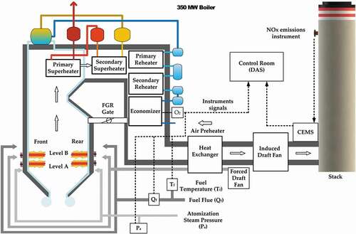
The experiment was carried out in a 350 MW industrial boiler with an opposite wall that burns heavy fuel oil with 24 burners installed in 12 cells with a secondary air register per burner pair. The unit has a balanced draft furnace and is of the subcritical, single reheat design. The maximum continuous rating (MCR) for steam flow output is 170 kg/cm² and 538°C is 1058 metric ton/h. Both main steam and hot reheat design temperatures are 538°C. Steam temperature control is achieved with flue gas recirculation (FGR). Figure 1 shows a simplified boiler scheme. Before the execution of the parametric test, some activities were carried out for combustion tunings such as preliminary tests, test planning, boiler inspection, burner balancing, sensitivity analysis of variables, and so on.

Figure 1. Boiler unit configuration.

Combustion tuning and preliminary tests

A combustion tuning was performed to balance the boiler stoichiometric status. Preliminary tests were accomplished at the three loads, 100%, 75%, and 50% using a combination of economizer oxygen excess ($O_2$), fuel temperature ($T_f$), steam atomization pressure ($P_a$), and FGR damper position. The oxygen excess was diverted by the total air flow to furnace boxes controlled by the forced draft fan. The fuel parameters such as temperature, pressure, and atomization were varied within a safe operating interval. The FGR gate was operated taking care not to exceed the boiler’s operating limits such as main steam temperature. Non-controllable variables (unit load, fuel mass flow ($Q_f$), steam temperature, etc.) were monitored to perform a sensitivity analysis on NOx emissions. Operating ranges for all variables were defined so as not to break any operational constraints limited by the boiler design.

Sensitivity analysis

Some ANN limitations are the quantity of data required, slow training process, overfitting, and hidden parameters within black box models. To reduce these limitations, it is necessary to omit irelevant data components in the model inputs to obtain reduced networks, small model structure, and minimal redundancy in the data. Selecting the appropriate input parameters for a neural network is known as feature selection, which means finding the most relevant variables for a specific goal. The sensitivity analysis is a method used to select variables and is often used to identify and rank relevant inputs.

According to (Evaluation of measurement data-Guide to the expression of uncertainty in measurement 2008), the partial derivatives of a model function $\mathrm{\partial }f/\mathrm{\partial }{x}_i$ are called sensitivity coefficients, describing how the output estimate $y$ varies with changes in the input values $x_1,x_2,\cdots ,x_N$. In particular, the change in $y$ produced by a small change $\mathrm{\Delta }{x}_i$ in the input estimate $x_i$ is given by ${\left(\mathrm{\Delta }y\right)}_i=\left(\mathrm{\partial }f/\mathrm{\partial }{x}_i\right)\left(\mathrm{\Delta }{x}_i\right)$. Instead of being calculated from the function f, sensitivity coefficients $\mathrm{\partial }f/\mathrm{\partial }{x}_i$ are sometimes determined experimentally when the function f is unknown. For experimental sensitivity analysis, the Morris method is commonly used, which has been used to test the impact of parameters. The Morris method evaluates the model output response for small changes in each input variable. The mean impact of a single variable from the complete dataset points of size M and N variables is presented as

(1) ${\mu }_k=\frac{1}{M}\sum _{k=1}^N\left|\frac{f\left(x_1,\cdots ,x_k+{\mathrm{\Delta }}_k,\cdots ,x_N\right)-f\left(x_1,\cdots ,x_N\right)}{{\mathrm{\Delta }}_k}\right|,$(1)

In the preliminary tests, a complete database was recorded where the input target variable $x_k$ was normally varied with time; however, small variations in all variables were unavoidable. To include these small uncontrollable changes in variables on sensitivity parameters ${\mu }_k$, the method developed in (Chen et al. 2020) was used. The problem is exchanged for the linear equation solution to find the ${\mu }_k$ parameters that include the variations of the inputs in the output. The common approach for the linear equation solution is to find the least-square solution to minimize the unfitted error referring to all used data points for sensitivity analysis. The input database created during the preliminary test has 2574 data points for each variable. The input data have seven different variables including controllable and uncontrollable boiler operating variables as shown in Table 1.

Table 1. Input variables for sensitivity analysis

Variables	Interval	Units
Economizer oxygen excess (O2)	0.4–7.2	%
Fuel mass flow (Qf)	41.7–80.5	Ton/hr
Flue gas recirculation (FGR)	0–100	%
Steam flow for temperature control (Qa)	0–70	Ton/hr
Steam atomization pressure (Pa)	12–16.5	Bar
Superheated steam temperature (Ts)	528–542	°C
Fuel temperature (Tf)	110–145	°C

The sensitivity analysis result is shown in Figure 2. The results indicate that the economizer oxygen excess has the highest sensitivity to NOx emissions, the top three highly sensitive variables are related to fuel/air ratio and flue gas temperature, which are involved with NOx generation.

Figure 2. Sensitivity analysis result of seven selected input variables.

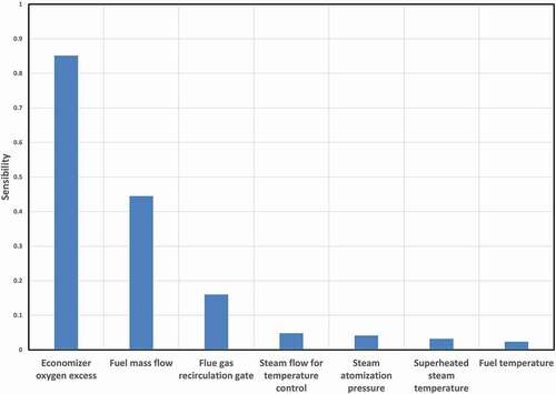
The steam flow for temperature control ($Q_a$), steam atomization pressure ($P_a$), superheated steam temperature ($T_s$), and fuel temperature ($T_f$) are the variables with the least sensitivity to NOx emissions. With the sensitivity analysis result, the number of input variables can be reduced by selecting only the three inputs with the highest sensitivity to the NOx emission model. Therefore, it was determined that the economizer oxygen excess ($O_2$), fuel mass flow ($Q_f$), and the flue gas recirculation (FGR) damper position are the most important variables with regard to NOx emissions.

Parametric test

Once the sensitivity analysis results had been determined, parametric tests were carried out at 50%, 75%, and 100% of the unit load to leave room for maneuver in the boiler process variables. There were 56 parametric tests including the baseline (BL) tests. For each test point, operational data was collected during at least 15 minutes intervals with 20 seconds sample time, once the stable operation was settled down. For data processing and test documentation, a data set from boiler data acquisition and the CEM system was collected automatically. The CEM system is installed in the boiler flue stack. Table 2 shows the 56 parametric tests used for NOx modeling.

Table 2. Parametric tests for NOx modeling

Test	O2	FGR	Qf	NOx ppm	Test	O2%	FGR%	Qft/h	NOx ppm
1BL	5.44	0	42.93	270.1	29	3.57	60	59.98	281.4
2	5.54	20	42.93	220.3	30	3.58	100	59.97	277.8
3	4.70	40	42.94	229.6	31	1.89	0	60.01	238.7
4	4.50	60	42.93	286.0	32	1.87	30	59.97	230.1
5	4.67	80	42.96	328.8	33	1.80	60	59.98	218.9
6	4.82	100	42.94	260.8	34	1.73	100	59.98	213.8
7	5.17	0	43.22	265.8	35BL	1.19	0	79.41	324.9
8	6.58	20	43.24	296.8	36	2.12	0	79.40	376.6
9	6.31	40	43.21	280.2	37	1.57	0	79.42	339.6
10	5.92	60	43.24	265.1	38	1.01	0	79.41	317.8
11	6.03	100	43.19	265.5	39	0.66	0	79.39	299.1
12	5.52	0	42.50	295.2	40	0.66	100	79.39	278.0
13	5.24	50	42.47	271.5	41	1.16	100	79.38	294.9
14	5.34	100	42.46	271.9	42	0.85	100	79.39	286.9
15	6.79	0	42.48	305.8	43	1.45	100	79.39	313.4
16	3.20	0	42.49	223.3	44	2.07	100	79.31	337.7
17	2.81	30	42.48	199.5	45	3.13	100	42.48	194.1
18	3.41	60	42.49	201.9	46	5.88	0	42.51	306.4
19	3.08	100	42.47	193.8	47	4.26	0	42.49	256.4
20	5.90	0	42.49	307.3	48	2.85	0	42.50	214.2
21	4.30	0	42.49	257.8	49	2.74	0	60.92	263.3
22	2.85	0	42.52	214.2	50	3.60	0	60.00	303.7
23BL	2.75	0	60.92	262.3	51	3.54	100	59.96	277.3
24	2.62	30	60.59	254.5	52	1.86	0	60.00	237.4
25	2.88	60	60.84	250.2	53	1.18	0	79.40	327.4
26	2.94	100	60.83	250.6	54	2.12	0	79.39	378.0
27	3.61	0	59.98	303.9	55	0.65	0	79.42	298.9
28	3.58	30	59.98	290.6	56	1.15	100	79.35	296.2

During the tests, different O₂ excess, FGR gate opening and unit load values were manipulated, while the other boiler parameters were adjusted according to the values established by the baseline.

The experimental data tests were divided into two subsets, one for the model development process (test 1–44) and the other for model evaluation (test 45–56). The test subset was selected considering include data from all the operation range of the input variables (O₂, FGR and O_f) 50%, 75% and 100% of the unit load.

Model selection

Model selection is a process where some model family is defined and in a second stage, the model structure is fixed. It is necessary to propose a candidate model family for the application. For NOx modeling, Bayesian-Gaussian, multilayer perceptron, and Volterra polynomial basis functions, ANNs were used as model families due to their capability to imitate nonlinear systems (Haykin 1999; Hornik, Stinchcombe, and White 1989).

A classical nonlinear system can be represented by

(2) $z_{t+1}=G\left(z_t,x_t\right),$(2)

(3) $y_t=h\left(z_t,x_t\right),$(3)

where $G\left(\cdot \right)$ is a vector of nonlinear functions, $h\left(\cdot \right)$ is a scalar nonlinear function, $z_t$ is the vector state, $y_t$ is the system output, and $x_t$ is the system input.

$ANN$ can uniformly approximate any continuous function including the nonlinear. The input-output $ANN$ model is presented in Figure 3, where $X_t$ is the input and the $o_t$ is the output.

Figure 3. Identification based on artificial neural networks.

The nonlinear system defined in (1) and (2) can be described by an equivalent nonlinear discrete system that can be characterized by a BG, an MLP, or a VPBF network model, that is,

(4) $o_t=f\left(X_t\right),$(4)

where $f\left(\cdot \right)$is a nonlinear function, ${\mathrm{X}}_{\mathrm{t}}=\left[x_1^t,x_2^t,\cdots ,x_n^t\right]$ the input vector and $y_t$ the output which represents a multiple-input single-output (MISO) system.

Bayesian-Gaussian ANN model

The Bayesian-Gaussian artificial neural network is a probabilistic model built with a neural network of five layers. The BG artificial neural network was proposed and developed in (Ye, Nicolai, and Reh 1998) under the Gaussian hypothesis and using Bayes’ theorem.

The BG model is built based mainly on the training data $\left(X_i,y_i\right),i=1,\cdots ,N$ set, where $N$ is the net order, $X_i$ is the sample input represented by a $n\times 1$ vector, and $y_i$ is the sample output. The BG model is based on the probability distribution of $Y\left(X\right)$ when the combined information sources $\left(X_i,y_i\right),i=1,\cdots ,N$ in known, details theory can be found in (Ye, Nicolai, and Reh 1998). The probability distribution of $Y\left(X\right)$ is approximately by

(5) $p\left(k\frac{1}{\sqrt{2\pi }\sigma \left(N\right)}{e}^{-\frac{1}{2}\frac{{\left(Y-o_B^t\left(N\right)\right)}^2}{\sigma {\left(N\right)}^2}}\right),$(5)

where $k$ is a normalizing constant independent of $Y$ and,

(6) $o_B^t\left(N\right)=\sigma {\left(N\right)}^2\sum _{i=1}^N{\sigma }_i^{-2}{y}_i,$(6)

(7) $\sigma {\left(N\right)}^{-2}=\sum _{i=1}^N{\sigma }_i^{-2}.$(7)

Assume that

(8) ${\sigma }_i^2={\sigma }_0^2{e}^{r_i},$(8)

where $r_i={\left(X_t-X_i\right)}^{T}D\left(X_t-X_i\right)$ and $D$ is input threshold matrix

(9) $D=\left[\begin{array}{ccc}{d}_{11}^{-2}& \cdots & 0\\ ⋮& \ddots & ⋮\\ 0& \cdots & d_{nn}^{-2}\end{array}\right],$(9)

and $d_{11},d_{22},\cdots ,d_{nn}$ are the parameters that have to be estimated.

The BG artificial neural network algorithm is built through Equations (5(5) $p\left(k\frac{1}{\sqrt{2\pi }\sigma \left(N\right)}{e}^{-\frac{1}{2}\frac{{\left(Y-o_B^t\left(N\right)\right)}^2}{\sigma {\left(N\right)}^2}}\right),$(5) –9(9) $D=\left[\begin{array}{ccc}{d}_{11}^{-2}& \cdots & 0\\ ⋮& \ddots & ⋮\\ 0& \cdots & d_{nn}^{-2}\end{array}\right],$(9) ) as shown in Figure 4, where the lines between layers without weight indication mean weight equal to one

Figure 4. The topology of Bayesian-Gaussian artificial neural networks.

The BG ANN can be naturally set with only the training data set. The network training is focused only on getting the adequate D matrix for some minimization error criteria.

Multilayer perceptron ANN model

MLPs are networks with one or more layers of artificial neurons between the input and output layers. MLP can be used for function approximation like the nonlinear system defined in Equation (4)(4) $o_t=f\left(X_t\right),$(4) . A three-layer MLP using the sigmoid activation function can approximate nonlinear function $f\left(\cdot \right)$. The structure of a three-layer MLP is shown in Figure 5, where $n$ is the neuron number in the input layer, $l$ the neuron number in the hidden layer, the weight matrices $W_t\in R^{n\times l}$ and $V_t\in R^l$, the input vector $X_t\in R^n$ and the output vector $o_M^t$.

Figure 5. MISO multilayer perceptron ANN.

Backpropagation (BP) learning is the most popular algorithm rule for performing supervised learning tasks. The optimization objective function is defined as the sum of the squared error $E_M^t$ between the actual network output $o_M^t$ and the desired output $y_t$ for all training pattern pairs $\left(X_t,y_t\right)$ for each $t=1,\cdots ,M$.

The $j$ neuron in the hidden layer is defined as the excitation function, corresponding to the $t$ sample

(10) $s_j^t=\sum _{i=1}^n{w}_{i,j}^t{x}_n^t+w_{n+1,j}^t,$(10)

each neuron has a sigmoidal activation function. The hidden layer output for the $j$ neuron is

(11) $h_j^t=\frac{1}{1+e^{-S_j^t}},$(11)

the neuron k excitation of the output layer is calculated analogously in the following form

(12) $r_M^t=\sum _{j=1}^l{v}_j^t{h}_j^t+v_{l+1}^t,$(12)

the output of the neuron k is expressed as

(13) $o_M^t=\frac{1}{1+e^{-r_M^t}},$(13)

finally, the criteria to be minimized in the sample $t$ is

(14) $E_M^t=\frac{1}{2}{\left(e_M^t\right)}^2=\frac{1}{2}{\left(y_t-o_M^t\right)}^2.$(14)

Volterra polynomial basis functions ANN model

The nonlinear system defined in Equation (4)(4) $o_t=f\left(X_t\right),$(4) can also be described by a VPBF model, which is an equivalent nonlinear discrete system.

It is assumed that the function $f\left(\cdot \right)$ is estimated by an ANN with only one layer (Wray and Green 1994) in the VPBF model, consisting of a linear combination of the basis functions.

(15) $o_V\left(X_t\right)=\sum _{i=1}^N{w}_i{\phi }_i\left(X_t\right),$(15)

where $X_t=\left[x_1^t,x_2^t,\cdots ,x_n^t\right]$, ${\phi }_k\left(X_t\right)$ is the basis function and $w_i$ the weight. Figure 6 shows a VPBF ANN structure.

Figure 6. Volterra polynomials basis function ANN.

There are a finite number of neurons in the network to guarantee some precision requirements (Haykin 1999). For this, it is necessary to implement a viable approach for selecting the best basis function set. The precision can be approximated by a tolerable neuron number, using Volterra polynomial functions. For $NOx$ modeling, $VPBF$ neural network is used. The nonlinear function $o_V\left(X_t\right)$ is

(16) $o_V\left(X_t\right)=w_1+w_2{x}_1^t+\cdots +w_{n+1}{x}_n^t+w_{n+2}{\left(x_1^t\right)}^2+w_{n+3}{x}_1^t{x}_2^t+\cdots +w_N{\left(x_n^t\right)}^k=\sum _{i=1}^N{w}_i{\phi }_i\left(X_t\right),$(16)

where $k$ is the polynomial order, and the set of the basis functions of the Volterra polynomial is

(17) $\left[{\phi }_1,{\phi }_2,\dots .,{\phi }_{n+1},{\phi }_{n+2},{\phi }_{n+3},\dots ,{\phi }_{N,}\right]\left(X_t\right)=\left[1,x_1^t,\dots ,x_n^t,{\left(x_1^t\right)}^2,x_1^t{x}_2^t,\dots .,{\left(x_n^t\right)}^k\right],$(17)

and the polynomial basis function number is given by

(18) $N=\frac{\left(n+k\right)!}{n!k!}.$(18)

Applying the VPBF ANN, the function $f\left(\cdot \right)$ is determined by

(19) $o_V\left(X_t\right)=\hat{f}\left(X_t\right)+e_V\left(X_t^k\right),$(19)

where $e_V\left(X_t^k\right)$ it is the approximation error.

When the order k increases$k$, the basis functions number $N$ increases exponentially. So, the aim is to determine the function $o_V\left(X_t\right)$ using an appropriate $ANN$, fitted to achieve that approximation precision is inside the required error limit. The model size and weights learning of the $ANN$ are also known as structure selection and parameter estimation, respectively.

Parameters estimation

Once the family and structure model are selected, the next step is parameter estimation to obtain the final model that best represents this family and structure model taking into account error minimization criteria. In this procedure stage, the error minimization criteria are proposed for the BG, MLP, and VPBF networks.

Bayesian-Gaussian ANN training

The BG network training is the updating of input threshold matrix $D$ where the $E_B$ in Equation (20)(20) $min{E}_B=mi{n}_D\frac{1}{2N}\sum _{i=1}^N{\left(y_i-o_B^i\right)}^2,$(20) is minimized,

(20) $min{E}_B=mi{n}_D\frac{1}{2N}\sum _{i=1}^N{\left(y_i-o_B^i\right)}^2,$(20)

where $y_i$ is the output training sample and $o_B^i$ is the network output sample.

The minimization method for BG ANN training selected is the Nelder-Mead simplex method (Nelder and Mead 1965).

Multilayer perceptron ANN training

The $E_M^t$ function can be minimized concerning the weight coefficient $w_{i,j}$ and $v_j$by applying the gradient-descent procedure. The $E_M^t$ gradient is,

(21) $\mathrm{\nabla }{E}_M^t=\left[\begin{array}{c}\frac{\mathrm{\partial }{E}_M^t}{\mathrm{\partial }{v}_j^t}\\ \frac{\mathrm{\partial }{E}_M^t}{\mathrm{\partial }{w}_{i,j}^t}\end{array}\right].$(21)

The gradient method consists of moving in the negative gradient direction, giving an update step of the weight coefficient values $w_{i,j}$ and $v_j$ with each training pattern pair $\left(X^t,y^t\right)$ i.e.

(22) $\left[\begin{array}{c}{v}_j^t\\ w_{i,j}^t\end{array}\right]=\left[\begin{array}{c}{v}_j^{t-1}\\ w_{i,j}^{t-1}\end{array}\right]-\eta \mathrm{\nabla }{E}_M^t,$(22)

where $\eta$ is a constant that is called the learning constant.

Volterra polynomial basis functions ANN training

To build a model for $NOx$ emissions with a given accuracy, it is first necessary to look for the basis functions that best represent (under some criteria) the nonlinear dynamics of $NOx$ emissions within a set of functions that is surely large due to the polynomial expansion nature and finally to estimate the model parameter for the reduced function set using some minimizing criteria.

The best basis function selection will be carried out offline applying the orthogonal least-squares approach (Billings, Korenberg, and Chen 1988) to define the more relevant VPBF set of basis functions for $NOx$ modeling.

Consider that disposes of a data set $\left(X_t,y_t,t=1,2,\cdots ,T\right)$ from system. Based on Equation (19)(19) $o_V\left(X_t\right)=\hat{f}\left(X_t\right)+e_V\left(X_t^k\right),$(19) , can be organized in vector form:

(23) $O_V\left(X\right)=\mathrm{\Phi }\left(X\right)W+E_V\left(X^k\right),$(23)

where $Y\in R^{T\ast 1}$is the output vector, is the weight vector, $W\in R^{T\ast 1}$ is the approximation error vector, and is the basis functions matrix

(24) $Y={\left[y_1{y}_2\cdots y_T\right]}^T,$(24)

(25) $W={\left[w_1{w}_2\cdots w_N\right]}^T,$(25)

(26) $E_V\left(X^k\right)={\left[e_V\left(x_1^k\right)e_V\left(x_2^k\right)\cdots e_V\left(x_T^k\right)\right]}^T,$(26)

(27) $\mathrm{\Phi }\left(X\right)=\left[\begin{array}{ccc}\begin{array}{c}{\phi }_1\left(x_1\right)\\ {\phi }_1\left(x_2\right)\\ \begin{array}{c}⋮\\ {\phi }_1\left(x_T\right)\end{array}\end{array}& \begin{array}{c}{\phi }_2\left(x_1\right)\\ {\phi }_2\left(x_2\right)\\ \begin{array}{c}⋮\\ {\phi }_2\left(x_T\right)\end{array}\end{array}& \begin{array}{cc}\begin{array}{c}\cdots \\ \cdots \\ \begin{array}{c}\ddots \\ \cdots \end{array}\end{array}& \begin{array}{c}{\phi }_N\left(x_1\right)\\ {\phi }_N\left(x_2\right)\\ \begin{array}{c}⋮\\ {\phi }_N\left(x_T\right)\end{array}\end{array}\end{array}\end{array}\right].$(27)

The weight vector $\mathrm{W}$ is generally getting with the minimum of the norm, that is,

(28) $\hat{W}=argmi{n}_{W}Y-\mathrm{\Phi }\left(X\right)W_2,$(28)

which is the least-squares solution.

The vector ${\mathrm{\Phi }}_i={\left[{\phi }_i\left(x_1\right),{\phi }_i\left(x_2\right),\cdots ,{\phi }_i\left(x_T\right)\right]}^T$, for $i=1,2,\cdots ,N$, form base vectors set, and the OLS solution $\hat{W}$, $\mathrm{\Phi }\left(X\right)\hat{W}$ is the projection of $\mathrm{Y}$ on the space generated by the basis functions $\left\{{\mathrm{\Phi }}_i\right\}$. The factorization of $\mathrm{\Phi }\left(X\right)$ matrix is:

(29) $\mathrm{\Phi }\left(X\right)=PQ,$(29)

where $P=\left[P_1,P_2,\cdots ,P_N\right]$ is a matrix of $T\times N$ and $P_1,P_2,\cdots ,P_N$ are orthogonal, and $Q$ is a unitary upper triangular matrix of $N\times N$.

The $P$ orthogonality property is useful for OLS solution, Equation (23)(23) $O_V\left(X\right)=\mathrm{\Phi }\left(X\right)W+E_V\left(X^k\right),$(23) can be written as

(30) $Y=PV+O_V\left(X\right),$(30)

(31) $W=Q^{-1}V,$(31)

where estimated $\hat{V}={\left[{\hat{v}}_1,{\hat{v}}_2,\cdots ,{\hat{v}}_N\right]}^T$ through

(32) ${\hat{v}}_i=\frac{Y^T{P}_i}{P_i^T{P}_i},parai=1,2,\cdots ,N.$(32)

So $Y-P{\hat{V}}_2$is minimal. The best W vector is

(33) $\hat{W}=Q^{-1}\hat{V}.$(33)

The classical Gram Schmidt method (Billings, Chen, and Korenberg 1989; Billings, Korenberg, and Chen 1988) is used to factorize the $\mathrm{\Phi }\left(X\right)$ matrix and estimating $\hat{W}$.

Note that $\sum _{i=1}^N{\hat{v}}_i^2{P}_i^T{P}_i/T$ is the variance of the basis function $i$, and $O^{T}O/T$ is the model error variance not included in $y_t$. Therefore, $v_i^2{P}_i^T{P}_i$ is the variance that corresponds to $P_i$ and the standardized error reduction due to $P_i$ is:

(34) $r_i=\frac{{\hat{v}}_i^2{P}_i^T{P}_i}{Y^{T}Y}.$(34)

This ratio is a simple algorithm to look for a relevant basis function subset.

Model evaluation

When models have been estimated or trained, they must be evaluated to determine whether or not they meet the requirements. In this work, the evaluation process is interactive and consists of estimating the model parameters with different model structures in BG, MLP, and VPBF networks families. For all three models, (BG, MLP, and VPBF) were developed 24 model structures varying the input number ($n$ in $X_t=\left[x_1^t,x_2^t,\cdots ,x_n^t\right]$ the input vector); and the neuron number in the hidden layer $l$ in the MLP networks and the order $k$ in VPBF networks.

The RMSE and the MAE (Chai and Draxler 2014) are the error metrics used to validate the models. These metrics were used for BG, MLP, and VPBF model validation.

The RMSE is defined by

(35) $RMSE=\sqrt{\frac{1}{n}\sum _{i=1}^n{e}_i^2,}$(35)

and the MAE is defined by

(36) $MAE=\frac{1}{n}\sum _{i=1}^n\left|e_i\right|,$(36)

$n$ is the sample number of model errors $e_i,i=1,2,\cdots ,n$.

The aim is to obtain a model that estimates $NOx$ emissions as accurately as possible according to RMSE and MAE error metrics criteria with a well-defined structure, easy implementation, and low computational cost.

Results

Considering that $NOx$ model is a system of multiple input single output (MISO) and due to the $NOx$ emissions being related to the $O_2$, $FGR$ and $Q_f$ boiler variables, the input vector is defined as

(37) $X_t=\left[x_1^t,\cdots ,x_1^{t-m_1},x_2^t,\cdots ,x_2^{t-m_2},x_3^t,\cdots ,x_3^{t-m_3}\right],$(37)

where $x_1=FGR$, $x_2=O_2$ and $x_3=Q_f$, $m_1$ is $x_1$ maximum delays, $m_2$ is $x_2$ maximum delays, $m_3$ is $x_3$ maximum delays and the output $y_t=NOx$ for BG, MLP, and VPBF models.

From Equation (4)(4) $o_t=f\left(X_t\right),$(4) the $NOx$ model can be represented by

(38) $y_t=f\left(x_1^t,\cdots ,x_1^{t-m_1},x_2^t,\cdots ,x_2^{t-m_2},x_3^t,\cdots ,x_3^{t-m_3}\right).$(38)

The model selection was made iteratively. Several model configurations were progressively developed and validated for BG, MLP, VPBF family models. The BG neural network was built using the experimental data training, the MLP ANN structure was settled with only one hidden layer, and the VPBF model was approximated by a single-layer neural network.

The data-based $NOx$ models were properly implemented taking into consideration 27 typical combinations of $m_1$, $m_2$ and $m_3$ with maximum delays from 0 to 2, each one in the input vector $\left[x_1^t,\cdots ,x_1^{t-m_1},x_2^t,\cdots ,x_2^{t-m_2},x_3^t,\cdots ,x_3^{t-m_3}\right]$ for BG, MLP, and VPBF models. The order of BG models was $N=2148$ which was defined based on the training sample number. The number of neurons in the hidden layer was $l=4,5,6$ in the MLP models. The VPBF models were tested for three different orders $k=2,3,4$. Because the polynomial expansion can grow intolerably, the VPBF models were reduced at the 20 most significant basis functions, using the criterion defined in Equation (34)(34) $r_i=\frac{{\hat{v}}_i^2{P}_i^T{P}_i}{Y^{T}Y}.$(34) , only when the number of basis functions $N$ was greater than 20.

For the development and validation of the models, the experimental samples were divided into two subsets. The first, called training data, contains 2148 samples, and the second, called validation data, contains 180 samples. The training data subset was used for parameter estimation of all model combinations, and the validation data subset was used to test the developed models using MAE and RMSE error metrics.

Table 3 shows the RMSE and MAE error metrics of the eight best BG models developed.

Table 3. The best BG model validation results

delays\metrics	MAE	RMSE
$m_1=0,m_2=0,m_3=2$	1.7318	2.5295
$m_1=1,m_2=1,m_3=2$	1.7783	2.5688
$m_1=0,m_2=1,m_3=2$	1.8055	2.6308
$m_1=2,m_2=1,m_3=2$	1.7941	2.6838
$m_1=1,m_2=0,m_3=2$	1.8535	3.1015
$m_1=2,m_2=1,m_3=2$	1.8727	3.1307
$m_1=0,m_2=0,m_3=1$	1.9731	3.6614
$m_1=0,m_2=0,m_3=0$	2.1310	3.9516

The BG model structure that provides the best $NOx$ prediction with $RMSE=2.5295$ and $MAE=1.7318$ was with $m_1=0$, $m_2=0$ and $m_3=2$, maximum delays in $x_1$, $x_2$ and $x_3$ respectively, which corresponds to the model input number $n=5$ whose input vector is $X_t=\left[x_1^t,x_2^{\mathrm{t}},x_3^{\mathrm{t}},x_3^{\mathrm{t}-1},x_3^{\mathrm{t}-2}\right]$. When $m_1,m_2=0,1$ and $m_3=2$ the errors are very close, but when $m_1,m_2=2$ and $m_3=0,1$ the error increases.

Table 4 shows the RMSE and MAE error metrics for the best-developed structures in the MLP models.

Table 4. The best MLP model validation results

delays\metrics	MAE	RMSE
$l=4,m_1=0,m_2=1,m_3=0$	12.5862	14.9220
$l=4,m_1=0,m_2=0,m_3=0$	12.7521	15.0319
$l=5,m_1=0,m_2=0,m_3=0$	12.7784	15.0764
$l=4,m_1=1,m_2=1,m_3=0$	12.7092	15.0909
$l=4,m_1=0,m_2=2,m_3=0$	12.7428	15.0915
$l=5,m_1=0,m_2=2,m_3=0$	12.7292	15.1188
$l=5,m_1=0,m_2=1,m_3=0$	12.8034	15.1529
$l=6,m_1=0,m_2=0,m_3=0$	12.8431	15.1556

The MLP model structure that provides the best $NOx$ prediction with $RMSE=14.9220$ and $MAE=12.5862$ was with $m_1=0$, $m_2=1$ and $m_3=0$ in $x_1$, $x_2$ and $x_3$ maximum delays, respectively, which corresponds to $n=4$ maximum size of $X_t=\left[x_1^t,x_2^{\mathrm{t}},x_2^{\mathrm{t}-1},x_3^t\right]$ input vector and $l=4$ four neurons in the hidden layer. However, when $l=4,6$ no large differences are observed in the metrics of the $NOx$ emissions prediction error, and in $m_1=m_2=m_3=0$ are good models.

Table 5 shows the RMSE and MAE error metrics for the best-defined structures for the VPBF models.

Table 5. VPBF model validation results

delays\metrics	MAE	RMSE
$k=4,m_1=0,m_2=0,m_3=0$	4.7878	6.6400
$k=3,m_1=2,m_2=0,m_3=0$	5.4737	6.8283
$k=4,m_1=0,m_2=1,m_3=0$	4.8961	6.8522
$k=4,m_1=2,m_2=0,m_3=0$	5.2456	6.8732
$k=4,m_1=2,m_2=1,m_3=0$	5.2864	6.9798
$k=3,m_1=0,m_2=2,m_3=0$	5.6431	7.0149
$k=3,m_1=0,m_2=1,m_3=1$	5.5755	7.0363
$k=3,m_1=0,m_2=0,m_3=0$	5.6123	7.0791

The VPBF model structure that provides the best $NOx$ prediction with $\mathrm{R}\mathrm{M}\mathrm{S}\mathrm{E}=6.64$ and $MAE=4.7878$ was with $m_1=0$, $m_2=0$ and $m_3=0$ without delays in $x_1$, $x_2$ and $x_3$, which corresponds to $n=3$ maximum size of $X_t=\left[x_1^t,x_2^t,x_3^{\mathrm{t}}\right]$ input vector and $k=4$ fourth-order system; whose maximum polynomial expansion number is $N=20$ basis functions.

In the results shown in Tables 3, 4, and 5, it is evident that the model family BG has better performance than the model family MLP and VPBF in NOx emission prediction. The predictions of NOx emissions, with validation data, of the best models achieved in the three structures BG, MLP, and VPBF are shown in Figure 7.

Figure 7. NOx measured and estimated in the model validation process.

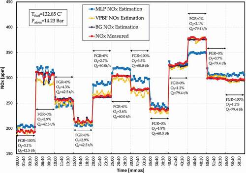
The three families of non-linear models BG, MLP, and VPBF can be used for modeling NOx emissions in an industrial boiler. The decision of which model structure is suitable for NOx modeling depends on specifications such as accuracy, computational cost, system variation over time, and so on.

Models with BG structure show the best precision but have a high computation cost because it depends on the number of samples in the training layer, which is usually large because the Gaussian hypothesis must be met. Models with VPBF structure would have a lower computation cost because the model is built with relatively few base functions. The structure and parameters of the BG and VPBF artificial neural networks can be modified relatively easily online, allowing the model to be adjusted and to compensate for potential deviations from the online model.

Conclusion

Currently, around the world, most energy is generated through fossil fuels, which generates large amounts of greenhouse gas. Polluting emissions are regulated, and it is necessary to measure them in order to control air pollution. An alternative approach was developed to predict NOx emissions from a utility boiler. A NOx model was built and evaluated using a data-based approach. The model structure proposed allows the estimation of NOx emissions caused by fossil fuel combustion, based on $O_2$ excess, fuel flue $Q_f$ and the FGR opening values, with good results. The NOx emission estimation can be improved by including other plant operation inputs correlated with NOx emissions and increasing the data training set. BG and VPBF neural networks are viable and cheap alternatives for emission quantification for prediction in industrial processes that pollute the environment. These algorithms can recycle plant operation data that contains valuable information about the internal operation of the boiler. This data has incalculable potential and is currently not exploited.

The black-box model approach does not require sophisticated algorithms or expensive equipment. It is the proper solution to the lack of emissions measurements and is a low-cost system for complete environmental monitoring of large pollution sources. Although these methods tend to produce lower-quality data, they can be used in a great number of localations, allowing an adequate pollution assessment in several places near power plants.

Disclosure statement

No potential conflict of interest was reported by the author(s).

Additional information

Notes on contributors

Guillermo Ronquillo-Lomeli

Guillermo Ronquillo-Lomeli was born in México City in 1968. He received the Ph.D. degree in Mechatronics from PICYT (interinstitutional postgraduate in science and technology), México in 2015, the M.S. in Automatic Control from the Autonomous University of Queretaro in 2002 and the B.S. degree in Electrical Engineering from Technological Institute of Queretaro in 1993. Guillermo has extensive experience in the design and manufacturing of special systems for the industry and is member of the National Mexican System of Research. His research interests include dynamic system modeling, control theory and system identification with application to energy.

Noé Amir Rodríguez-Olivares

Noé Amir Rodríguez-Olivares received the Ph.D. Degree in Mechatronics from PICYT (interinstitutional postgraduate in science and technology), Mexico in 2019, the Master Degree in Mechatronics also from the PICYT in 2014, and Mechatronics Engineering from the Technological Institute of Poza Rica, Veracruz, Mexico, in 2011. He works for CIDESI (Engineer Center and Industrial Development) and the Anahuac Queretaro University; he is a member of the National Mexican System of Research (SNI); his main area of interest is the algorithm in embedded systems for instrumentation and digital control.

Leonardo Barriga-Rodríguez

Leonardo Barriga-Rodríguez received the Ph.D. degree in Mechatronics from PICYT (interinstitutional postgraduate in science and technology), México in 2014, the Master Degree in Mechatronics also from the PICYT in 2009, and Computer Systems from the Technological Institute of Jiquilpan, Michoacán México in 2004. He works for CIDESI (Engineering Center and Industrial Development), as research professor in the Electrical and electronic engineering department; he is a member of the National Mexican System of Research; his research interests include development of algorithms in artificial intelligence and computer vision.

Antonio Ramírez-Martínez

Antonio Ramírez-Martínez received a Ph.D. degree in Mechatronics from PICYT (interinstitutional postgraduate in science and technology), México in 2015, the M.S. in mechanical Design in 2002 from PICYT and the B.S. degree in mechanics with a specialty in thermal from Technological Institute of Celaya in 1991. His research interest is on robotic inspection, particularly in Pipeline inspection with instrumented pigs, and participating in projects for thermal cycles of electricity generation.

Jorge Alberto Soto-Cajiga

Jorge Alberto Soto-Cajiga was born in Queretaro México in 1980. He received the Ph.D. degree in Mechatronics from PICYT (interinstitutional postgraduate in science and technology) in 2012, the M.S. in Mechatronics also from the PICYT in 2006 and the B.S. degree in Electrical Engineering from Technological Institute of Queretaro in 2003. Jorge has extensive experience in development of special electronics systems for the industry, actually is research professor at the center for engineering and industrial development, responsible for the instrumented equipment laboratory and his areas of interest are in the development of instrumented equipment for inspection, real-time signal processing implemented in hardware and development of electronic systems for specific application.

Luciano Nava-Balanzar

Luciano Nava-Balanzar received the Ph.D. Degree in Mechatronics from PICYT (interinstitutional postgraduate in science and technology), México in 2016, the Master Degree in Mechatronics also from the PICYT in 2010 and Control and Instrumentation Engineering from the Technological Institute of San Juan del Río, Querétaro, Mexico, in 2006. He works for CIDESI (Engineer Center and Industrial Development), as research professor in the area of Robotics and Instrumentation, and his research interests include; Electronics, design electronic, embedded system, signal processing algorithms and electronic architecture development for underwater robots.

References

- Billings, S. A., S. Chen, and M. J. Korenberg. 1989. Identification of MIMO non-linear systems using a forward-regression orthogonal estimator. Int. J. Control 49 (6):2157–89. doi:https://doi.org/10.1080/00207178908559767.
- Billings, S. A., M. J. Korenberg, and S. Chen. 1988. Identification of non-linear output-affine systems using an orthogonal least-squares algorithm. Int. J. Syst. Sci. 19 (8):1559–68. doi:https://doi.org/10.1080/00207728808964057.
- Bowman, C. T. 1992. Control of combustion-generated nitrogen oxide emissions: Technology driven by regulation. Symp. Int. Combust 24 (1):859–78. doi:https://doi.org/10.1016/S0082-0784(06)80104-9.
- Chai, T., and R. R. Draxler. 2014. Root mean square error (RMSE) or mean absolute error (MAE)? – Arguments against avoiding RMSE in the literature. Geosci. Model. Dev. 7 (3):1247–50. doi:https://doi.org/10.5194/gmd-7-1247-2014.
- Chen, S., Y. Ren, D. Friedrich, Z. Yu, and J. Yu. 2020. Sensitivity analysis to reduce duplicated features in ANN training for district heat demand prediction. Energy AI 2:100028. doi:https://doi.org/10.1016/j.egyai.2020.100028.
- Cheng, C. M., Z. K. Peng, W. M. Zhang, and G. Meng. 2017. Volterra-series-based nonlinear system modeling and its engineering applications: A state-of-the-art review. Mech. Syst. Signal Process 87:340–64. doi:https://doi.org/10.1016/j.ymssp.2016.10.029.
- Cybenko, G. 1989. Approximation by superpositions of a sigmoidal function. Math. Control Signals Syst. 2 (4):303–14. doi:https://doi.org/10.1007/BF02551274.
- Evaluation of measurement data-Guide to the expression of uncertainty in measurement. 1st ed. Joint Committee for Guides in Metrology. 2008. https://www.bipm.org/utils/common/documents/jcgm/JCGM_100_2008_E.pdf
- Funahashi, K.-I. 1989. On the approximate realization of continuous mappings by neural networks. Neural Networks 2:183–92. doi:https://doi.org/10.1016/0893-6080(89)90003-8.
- Han, H., Q. Chen, and J. Qiao. 2010. Research on an online self-organizing radial basis function neural network. Neural Comput. Appl. 19 (5):667–76. doi:https://doi.org/10.1007/s00521-009-0323-6.
- Haykin, S. 1999. Neural networks: A comprehensive foundation. Vol. 13, 2nd ed. New York: Prentice Hall International. doi:https://doi.org/10.1017/S0269888998214044.
- Hocking, W. R., R. Johnson, and P. T. Flowers. 2002. Application of advanced process control with neural networks to control power plant emissions. ISA TECH/EXPO Technol. Updat. 424–425:190–96.
- Hornik, K., M. Stinchcombe, and H. White. 1989. Multilayer feedforward networks are universal approximators. Neural Networks 2 (5):359–66. doi:https://doi.org/10.1016/0893-6080(89)90020-8.
- Ikonen, E., K. Najim, and U. Kortela. 2000. Neuro-fuzzy modelling of power plant flue-gas emissions. Eng. Appl. Artif. Intell. 13 (6):705–17. doi:https://doi.org/10.1016/S0952-1976(00)00054-3.
- Iliyas, S. A., M. Elshafei, M. A. Habib, and A. A. Adeniran. 2013. RBF neural network inferential sensor for process emission monitoring. Control Eng. Pract. 21 (7):962–70. doi:https://doi.org/10.1016/j.conengprac.2013.01.007.
- Kassam, S. A., and I. Cha. 1993. Radial basis function networks in nonlinear signal processing applications. Proc. 27th Asilomar Conf. Signals, Syst. Comput. 2:1021–25. IEEE Comput. Soc. Press. doi:https://doi.org/10.1109/ACSSC.1993.342415.
- Li, K., S. Thompson, and J. Peng. 2002. GA based neural network modeling of NOX emission in a coal-fired power generation plant. IFAC Proc. Vol. 35 (1):281–86. doi:https://doi.org/10.3182/20020721-6-ES-1901.01198.
- Liu, G. P. 2001. Nonlinear identification and control: A neural network approach. London; New York: Springer.
- Liu, Y., and C. Peng. 2009. Time-variation nonlinear system identification based on Bayesian-Gaussian neural network. Int. Conf. Nat. Comput. 1:353–57. IEEE. doi:https://doi.org/10.1109/ICNC.2009.187.
- Luo, W., and S. A. Billings. 1995. Adaptive model selection and estimation for nonlinear systems using a sliding data window. Signal Processing 46 (2):179–202. doi:https://doi.org/10.1016/0165-1684(95)00081-N.
- Luo, W., S. A. Billings, and K. M. Tsang. 1996. On-line structure detection and parameter estimation with exponential windowing for nonlinear systems. Eur. J. Control 2 (4):291–304. doi:https://doi.org/10.1016/S0947-3580(96)70054-7.
- Nelder, J. A., and R. Mead. 1965. A simplex method for function minimization. Comput. J. 7 (4):308–13. doi:https://doi.org/10.1093/comjnl/7.4.308.
- Ronquillo-Lomeli, G., G. Herrera-Ruiz, J. Ríos-Moreno, I. Ramirez-Maya, and M. Trejo-Perea. 2018. Total suspended particle emissions modelling in an industrial boiler. Energies 11 (11):3097. doi:https://doi.org/10.3390/en11113097.
- Safdarnejad, S. M., J. F. Tuttle, and K. M. Powell. 2019. Dynamic modeling and optimization of a coal-fired utility boiler to forecast and minimize NOx and CO emissions simultaneously. Comput. Chem. Eng. 124:62–79. doi:https://doi.org/10.1016/j.compchemeng.2019.02.001.
- Schmidt, C. A., S. I. Biagiola, J. E. Cousseau, and J. L. Figueroa. 2014. Volterra-type models for nonlinear systems identification. Appl. Math. Model. 38 (9–10):2414–21. doi:https://doi.org/10.1016/j.apm.2013.10.041.
- Shi, Y., W. Zhong, X. Chen, A. B. Yu, and J. Li. 2019. Combustion optimization of ultra supercritical boiler based on artificial intelligence. Energy 170:804–17. doi:https://doi.org/10.1016/j.energy.2018.12.172.
- Sjöberg, J., Q. Zhang, L. Ljung, A. Benveniste, B. Delyon, P.-Y. Glorennec, H. Hjalmarsson, and A. Juditsky. 1995. Nonlinear black-box modeling in system identification: A unified overview. Automatica 31 (12):1691–724. doi:https://doi.org/10.1016/0005-1098(95)00120-8.
- Smrekar, J., P. Potočnik, and A. Senegačnik. 2013. Multi-step-ahead prediction of NOx emissions for a coal-based boiler. Appl. Energy 106:89–99. doi:https://doi.org/10.1016/j.apenergy.2012.10.056.
- Song, J., C. E. Romero, Z. Yao, and B. He. 2017. A globally enhanced general regression neural network for on-line multiple emissions prediction of utility boiler. Knowledge-Based Syst. 118:4–14. doi:https://doi.org/10.1016/j.knosys.2016.11.003.
- Tuttle, J. F., L. D. Blackburn, K. Andersson, and K. M. Powell. 2021. A systematic comparison of machine learning methods for modeling of dynamic processes applied to combustion emission rate modeling. Appl. Energy 292:116886. doi:https://doi.org/10.1016/j.apenergy.2021.116886.
- Tuttle, J. F., L. D. Blackburn, and K. M. Powell. 2020. On-line classification of coal combustion quality using nonlinear SVM for improved neural network NOx emission rate prediction. Comput. Chem. Eng. 141:106990. doi:https://doi.org/10.1016/j.compchemeng.2020.106990.
- Tuttle, J. F., R. Vesel, S. Alagarsamy, L. D. Blackburn, and K. Powell. 2019. Sustainable NOx emission reduction at a coal-fired power station through the use of online neural network modeling and particle swarm optimization. Control Eng. Pract. 93:104167. doi:https://doi.org/10.1016/j.conengprac.2019.104167.
- Wray, J., and G. G. R. Green. 1994. Calculation of the Volterra kernels of non-linear dynamic systems using an artificial neural network. Biol. Cybern. 71 (3):187–95. doi:https://doi.org/10.1007/BF00202758.
- Ye, H., R. Nicolai, and L. Reh. 1998. A Bayesian–Gaussian neural network and its applications in process engineering. Chem. Eng. Process 37 (5):439–49. doi:https://doi.org/10.1016/S0255-2701(98)00051-8.
- Zeng, X., H. Zhao, and W. Jin. 2012. Nonlinear plant identifier using the multiple adaptive RBF network convex combinations. Adv. Comput. Sci. Inf. 2:185–91. Berlin Heidelberg: Springer Verlag. doi:https://doi.org/10.1007/978-3-642-30223-7_30.
- Zhou, H., and K. Cen. 2018. Combustion optimization based on computational intelligence. Singapore: Springer Singapore. doi:https://doi.org/10.1007/978-981-10-7875-0.