Computational modeling of woodstove pollutants in dilution tunnels

ABSTRACT

The computational modeling of the dilution tunnels used for experimental measurement of the woodstove pollution was presented. Two EPA-approved test labs for residential wood heat appliances, referred to as Lab-1 and Lab-2 dilution tunnels were simulated. The Ansys-Fluent software was enhanced with the addition of user-defined functions (UDF) and was used to simulate the airflow velocity, temperature, and particle concentration in the dilution tunnels. Particular attention was given to the variation of concentration profile at the test section and its uniformity. The simulation results suggested that roughly uniform or somewhat non-uniform particle concentrations entering from the woodstove stack into the dilution tunnel led to the uniform concentration at the outlet of the tunnel. This is particularly the case for the Lab-1 dilution tunnel. However, for the Lab-2 dilution tunnel, a highly non-uniform concentration at the woodstove stack outlet flowing at a high velocity into the dilution tunnel led to a non-uniform profile for the particle concentration at the test section. For this case, replacing the second elbow that is downstream from the mixing section with a tee reduced the nonuniformity of the concentration profile at the tunnel outlet.

Implications: This study numerically investigated two dilution tunnels used in EPA-approved test labs. The dilution tunnel is used to dilute and cool the exhaust flow of the woodstove’s stack. A properly working dilution tunnel provides a uniform concentration at the test section. Under different conditions, particulate matter (PM) laden turbulent flows in the tunnels are simulated to assess the dilution tunnel’s performance. The goal is to understand the conditions that the dilution tunnels provide uniform concentration at their test section. The presented results suggest that using a tee instead of an elbow would enhance mixing and the chance for generating uniform concentration at the test section.

Introduction

About 40% of the world’s population depends on biomass-based appliances for cooking and heating, and woodstoves are among the mostly used biomass-based appliances, especially in rural areas (Birol, 2010; Eilenberg et al. 2018). Studies on performances of residential wood combustion are of interest due to their effects on environmental air pollution and human health (Ochieng, Tonne, and Vardoulakis 2013; Sevault et al. 2017). For accessing the performance of woodstoves as an example of residential wood combustion, the exhaust particulate matter (PM) emission needs to be measured. Particulate matter (PM) emitted from the woodstove’s stack varies with time. Due to the transient nature of stack flow, emission measurements at the outlet of the woodstove’s stack are challenging (Boman et al. 2005). Accurate measurement is only possible when the exhaust flow of the stove is roughly uniform and diluted with lower temperature airflow. A dilution tunnel is typically used to dilute and cool the exhaust flow and generate a uniform condition in the test section by mixing exhaust gas with the ambient air, typically with a dilution factor of 10 to 25. The exhaust flow after the dilution tunnel reaches a lower temperature, with particle concentration in the measuring range and a dewpoint usually lower than ambient temperature. The PM concentrations can then be measured over a longer period, and the corresponding steady particle size distribution could be evaluated (Boman et al. 2005; Obaidullah, Svend, and Jacques 2018; Tissari et al. 2007). The dilution tunnel is used to dilute the airflow that enables constant volume sampling (CSV) (Boman et al. 2005). Dilution tunnel with CSV was first introduced to study the emission of the internal combustion engine under controlled conditions (Habibi 1970). For the PM emission measuring of woodstoves, the dilution tunnel that has been standardized by US Environmental Protection Agency (US EPA) as Method 5 G has been used (US Environmental Protection Agency 2000).

More recently, the US EPA updated the regulatory test method to use ASTM-E2515-11 (“2515”) (ASTM E2515-11 2017). Method 5 G tunnels use mixing baffles as shown in Figure 1, while 2515 does not; other than this, the two designs are similar. The US EPA and others have assumed that 2515 provides complete mixing of the stack flow and dilution air despite the lack of mixing baffles. However, to our knowledge, this has never been modeled or experimentally confirmed other than by the use of the “paired sample train” precision measurements required by the method, which requires the difference between the two measurements for an entire test run to be within 7.5%. In addition, recent work with real-time PM measurement methods (Allen et al. 2022) has shown that there can be transient non-uniform PM mixing events in a 2515 tunnel.

Figure 1. Method 5G dilution tunnel schematic (US Environmental Protection Agency 2000).

Figure 1 shows the schematic of a Method 5 G dilution tunnel (US Environmental Protection Agency 2000). The stove stack’s exhaust flow is mixed with the clean surrounding air in the collection hood and the mixing section of the tunnel. Note that the baffles shown here for EPA Method 5 G in Figure 1 are no longer used in the current EPA regulatory test method (ASTM2515). Here, the sampling system is implemented in the vertical testing section of the tunnel, where the flow is assumed to be uniformly mixed. An emission sampling system (PM measuring instruments) collects the aerosol concentration data in the test section of the dilution tunnel for an extended time and provides near-real-time data (Cong et al. 2017).

Some studies in the literature focus on the sampling system as an essential part of the dilution tunnel. Several studies have been done on the particle penetration in bent flows to evaluate the sampling system’s performance (Brockmann 2001; Peters and Leith 2004; Pui, Romay-Novas, and Liu 1987; Sun et al. 2013; Wilson et al. 2011). These studies investigated the effect of sampling tube configuration, including the bent angle and the characteristic aerosols-laden flow. Many of these studies mainly focused on the discrepancy between particle concentration at the inlet and outlet caused by particle deposition on the bend. In addition to the experimental studies, there are some numerical simulations for flow through bends (Breuer, Tarik Baytekin, and Matida 2006; Quek, Wang, and Ray 2005; Tsai and Pui 1990).

In the presented investigation, three specific configurations for the dilution tunnel are studied, based on existing installations at two EPA-certified residential wood heater appliance test laboratories. All the considered cases are full flow dilution (Obaidullah, Svend, and Jacques 2018), which means all the exhaust flow from the combustion appliance goes to the collection hood and is mixed with ambient air. The main focus of the study is on the pollutant particle concentration in the test section. As noted before, a dilution tunnel configuration that provides uniform concentration at the outlet (test section) is a suitable configuration for the experimental study. It should be noted that the considered dilution tunnels in this study do not have baffles in the mixing section shown in the schematic in Figure 1. As noted before, these baffles are no longer used in the new ASTM2515 testing standards.

Numerical simulation methods

In the present study, the volume flow rate of the tunnel is 0.2832 $\frac{m^3}{s}$ (600 CFM) which corresponds to the turbulent flow condition in the tunnel. The pollutant particle’s dimension is around 0.5 to 1 μm, and the mass fraction of the particles is typically low. Pollutants with low concentrations transported with airflow in the tunnel have negligible effects on the thermophysical properties of the turbulent airflow. Therefore, a one-way coupling between pollutants and turbulent airflow can be assumed. Among the several available methods to simulate two-phase particle-laden flows, in the present study, the pollutants are treated as a passive scalar that is transported by the mean airflow and diffuses by turbulence. The stove combustion products enter the dilution tunnel at the stack inlet, as shown in Figure 1. The Ansys-Fluent code is used in this study. The validation and limitation of the code were studied earlier (He and Ahmadi 1999; Mofakham and Ahmadi 2019, 2020; Tian and Ahmadi 2007). In addition, a 2D model of the tunnel mid-section is considered for the computational simulations. The three-equation transition k-kl-ω turbulence model (Walters and Cokljat 2008) was used for analyzing the turbulent flow condition in the tunnel. This model uses the Boussinesq eddy viscosity hypothesis to determine the Reynolds stress tensor (Walters and Cokljat 2008). The model solves three transport equations: turbulence kinetic energy, k, laminar kinetic energy, kl, and specific dissipation rate, ω. The simulations are performed using the coupled algorithm for pressure-velocity coupling. The momentum, scalar, and temperature equations were discretized with a second-order method. A user-defined function (UDF) for including the turbulence dispersion was developed and added to the code to solve the diffusion equation for the particle concentration in these simulations. The mesh is generated with ANSYS meshing. A minimum of 50,000 cell grids was used for all cases, which was refined near the walls to ensure $y^{+}$< 1.

Results

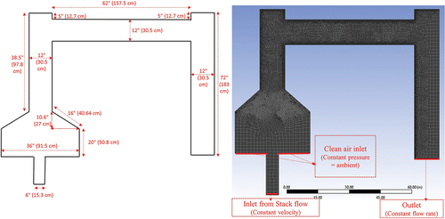
In this study, three different tunnel configurations are considered. First, for each case, the schematic of the domain and boundary conditions are presented, followed by the discussion of the simulation results. The high-temperature air and smoke enter from the stack inlet, mixes with the clean surrounding air, and enter the tunnel. Boundary conditions of ambient pressure and temperature are assumed for the surrounding air hood inlet. A constant velocity boundary condition is assumed for the stack inlet that varies for different cases. The outlet is assumed to have a constant volume flow rate of 0.2832 $\frac{m^3}{s}$ (600 CFM) that was used in the experimental study. The stack inlet has a constant temperature of T = 573 K, and the surrounding air hood inlet has a temperature of T = 300 K. All walls are assumed to be adiabatic.

The presented results include the velocity and concentration contours and concentration profile plots. For the study of the smoke particle concentration in the tunnel and, particularly, at the outlet of the tunnel, the passive scalar is considered a nondimensional parameter that is a fraction of the inlet concentration. Here, the user-defined scalar, which is the particle concentration, is prescribed at the tunnel inlet. The maximum value at the inlet is assumed to be 1, so that the results can be scaled easily to any other given inlet concentration.

Several simulations were performed for the baseline Lab-1 dilution tunnel. The simulation results indicated that the mixing was pretty good. A uniform or non-uniform concentration entering from the smokestack led to a uniform concentration profile at the dilution tunnel outlet (test section). Therefore, attention was given to the Lab-2 tunnel for which some non-uniform concentration profiles at the test section under certain conditions were experimentally observed.

Uniform concentration for the stack flow at the inlet

Two different dilution tunnel configurations are considered in this section. The stack flow entering the dilution tunnel is assumed to have a uniform concentration of particles with a uniform velocity of V = 1.5 m/s.

Lab-1 dilution tunnel with tees

Figure 2 shows the Lab-1 dilution tunnel configuration and the corresponding computational grids. Using the provided dimensions, the computational geometry was created in Ansys Geometry. Then domain meshing was carried out by the ANSYS meshing to generate the computational grids. For evaluating the performance of the tunnel, the contour of the airflow velocity, temperature, turbulence intensity, and particle concentration are presented and discussed in this section.

Figure 2. Lab-1 dilution tunnel configuration and computational grids.

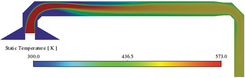
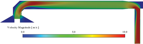
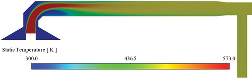
The temperature and velocity contours of the airflow throughout the tunnel are presented in Figure 3. Stove stack flow enters the tunnel with a temperature of T =573 k. The temperature at the outlet is uniform and is close to the temperature of the surrounding air at the inlet (300k).

Figure 3. Lab-1 Velocity magnitude contours (left) and the temperature contours (right) for stack inlet velocity and temperature of V=1.5 m/s and T=573K.

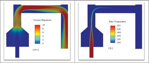
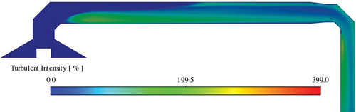
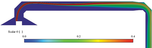
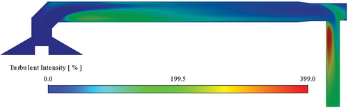
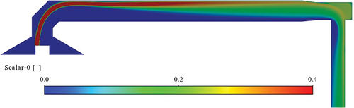
Figure 4 presents the contours of turbulent intensity and particle concentration. It is seen that the turbulent intensity increases after the 90-degree tee sections, and the flow, especially at the test section of the tunnel, has a high turbulent intensity, which implies good mixing. Figure 4 proves that, for this configuration and boundary condition, the particle concentration is uniform at the outlet of the Lab-1 dilution tunnel. Figure 5 shows the particle concentration profile at the outlet of the tunnel, further confirms this conclusion, and clearly shows that the outlet concentration is uniform. Here the average deviation from the mean value is 5%.

Figure 4. Lab-1 Turbulent intensity contours (left) and the particles concentration contours (right). Non-dimensional particle concentration at the stack inlet is assumed to equal one.

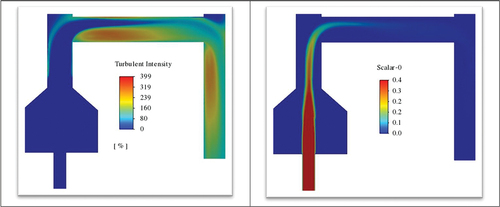
Figure 5. Lab-1 particle concentration profiles at the tunnel outlet. Non-dimensional particle concentration at the stack inlet is one.

Lab-2 dilution tunnel with elbows

Figures 6 and 7 show the Lab-2 dilution tunnel configuration with 90-degree elbows. Similar to Case 1 for Lab-1 dilution tunnel, the computational geometry was created in Ansys Geometry, and then domain meshing was carried out by the ANSYS meshing. For this case, a uniform concentration of particles with a stack flow velocity of V = 1.5 m/s is considered for the stove stack inlet boundary conditions into the dilution tunnel.

Figure 6. Lab-2 dilution tunnel configuration with elbows.

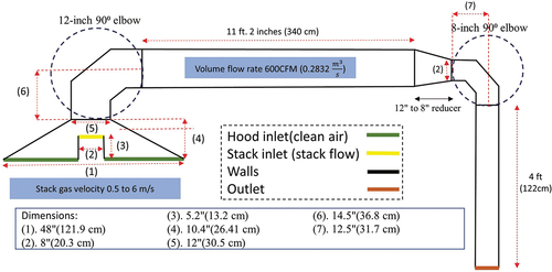
Figure 7. Lab-2 tunnel elbow and reducer dimensions.

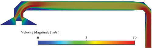
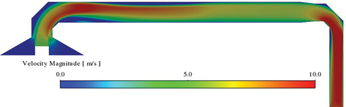
Figure 8 shows the airflow velocity contours in the Lab-2 dilution tunnel. It is seen that the velocity magnitude increases after the elbow as air enters the dilution tunnel. In addition, after the second elbow, the air velocity increase as the cross-section of the outlet pipe is smaller than the body of the dilution tunnel.

Figure 8. Lab-2 tunnel with elbows. Velocity magnitude contours at the midsection of dilution tunnel for V=1.5 m/s at stack inlet.

Figure 9 shows the particle concentration contours in the Lab-2 dilution tunnel. For this configuration, with an assumption of uniform smoke particle concentration at the inlet, it is seen that the particle enters the dilution tunnel in a uniform band and then disperse in the tunnel due to turbulent dispersion. The particle concentration becomes roughly uniform halfway through the tunnel and stays uniform through the outlet.

Figure 9. Lab-2 with elbows. Particle concentration contours at the midsection of the dilution tunnel. Here a uniform concentration at the stack inlet to the tunnel is assumed.

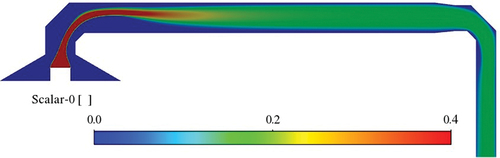
Figure 10 shows the particle concentration profile at the outlet of the tunnel. This figure clearly shows that the concentration is relatively uniform at the outlet. Here the average deviation from the mean value, not including the wall values, is 9%. That is, a uniform concentration entering the Lab-2 dilution tunnel would lead to a uniform concentration at the test section.

Figure 10. Lab-2 with elbows. Particle concentration profiles at the outlet. Here a uniform concentration at the stack inlet to the tunnel is assumed.

Non-uniform concentration at the stack inlet

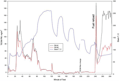
As noted before, simulation results showed that the uniform inlet concentration would result in uniform outlet concentration. However, the experimental data for the Lab-2 tunnel exhibited a non-uniform concentration at the test section under certain conditions. The sample measured data are shown in Figure 11. Here the red and black lines are the concentration measured by two probes at the test section. It is seen that most of the time, the two probes measure the same concentration indicating a uniform profile at the test section. However, for specific periods (between 35–50 and 245–290 minutes of testing), the concentration at the test section becomes highly non-uniform.

Figure 11. Experimental data for Lab-2 tunnel concentration and stack temperature.

The computer model predicts that if the concentration entering the dilution tunnel is roughly uniform, it stays uniform at the test section. Therefore, to provide insight into the reasons for the observed non-uniform concentrations at the test section in Figure 11, a series of simulations for the Lab-2 tunnel were performed. Here it is assumed that the concentration of the stack flow entering the dilution tunnel is highly non-uniform. In addition, two designs for the Lab-2 tunnel are studied. One design is with two 90 degree elbows (same configuration as the previously presented), and the other is with the elbow downstream of the mixing section replaced with a tee. Finally, both designs are simulated, and the results are compared.

Lab-2 dilution tunnel with two elbows

Similar to the previous case, Figures 6 and 7 show the Lab-2 dilution tunnel configuration with two 90 degree elbows. In this simulation, the stack flow’s inlet velocity is assumed to be 6 m/s to examine the high particle concentration situation. Large firebox capacity heater appliances like the indoor wood furnace used in Figure 11 have higher maximum burn rates than wood stoves and thus higher stack velocities for the same stack diameter.

For assessing the potential for non-uniform concentration profile at the test section, the particle concentration distribution at the stack inlet to the tunnel is assumed to be non-uniform. To provide a sharp contrast, the concentration at the left corner of the stack flow was assumed to be the highest at 1 and zero on the rest of the section.

Figure 12 shows the velocity magnitude contours in the dilution tunnel. Again, it is seen that the high-velocity flow from the stack penetrates the dilution tunnel, and the speed increases in the outlet pipe due to its smaller size.

Figure 12. Lab-2 configuration with two elbows. Velocity magnitude contours at the midsection of the dilution tunnel. Here the stack inlet velocity is V=6m/s.

Figure 13 shows the contours of the turbulence intensity in the dilution tunnel. As expected, it proves that the turbulence intensity increases after the bend in the dilution tunnel, especially after sharp edges, which provide good mixing.

Figure 13. Lab-2 configuration with two elbows. Turbulence intensity contours at the midsection of the dilution tunnel.

Figure 14 shows the temperature contours in the tunnel. The stove’s exhaust flow enters the tunnel with a temperature of T = 573k. Surrounding air enters the tunnel with T = 300k. From the temperature contours, it is concluded that the flow at the test section is at a uniform temperature of T = 490k. This observation suggests that if the concentration at the stack outlet is uniform, the concentration at the tunnel test section also becomes uniform even for this high stack velocity.

Figure 14. Lab-2 configuration with two elbows. Temperature contours at the midsection of the dilution tunnel. Here the stack inlet temperature is T=573k.

The most critical parameter of interest is the particle concentration in the dilution tunnel, mainly in the test section. Figure 15 shows the concentration contours in the tunnel. Here it is assumed that the concentration at the stack inlet to the tunnel is highly non-uniform. The concentration near the outer edge of the stack is highest and negligible in the rest of the section. Figure 15 shows that, although the mixing in the dilution tunnel is reasonably strong, the flow at the test section (at the outlet of the tunnel) is not fully mixed, and the concentration profile is non-uniform.

Figure 15. Lab-2 configuration with two elbows. Particle concentration contours at the midsection of the dilution tunnel. Here a highly non-uniform concentration at the stack inlet to the tunnel is assumed.

To improve the performance of the tunnel, enhance mixing and provide a more uniform concentration at the test section, the turbulence intensity in the flow should be increased with a modification of the tunnel. Here the influence of a tee connection downstream of the mixing section instead of the right elbow is explored.

Lab-2 dilution tunnel with a tee

Here the Lab-2 tunnel is modified by replacing the elbow on the right side of the tunnel with a tee. The geometry of the tee is shown in Figure 16.

Figure 16. Lab-2 tee configuration.

Figure 17 shows the velocity magnitude contours in the Lab-2 tunnel with a tee. The velocity contours are comparable to those shown in Figure 12.

Figure 17. Lab-2 configuration with elbow and tee. Velocity magnitude contours at the midsection of the dilution tunnel. Here the stack inlet velocity is V=6m/s.

Figure 18 shows the turbulence intensity contours in the modified Lab-2 tunnel. Again, it is seen that the turbulence intensity markedly increases after the tee section.

Figure 18. Lab-2 configuration with elbow and tee. Turbulence intensity at the midsection of the dilution tunnel.

Figure 19 shows the temperature contours in the tunnel. Accordingly, the temperature at the test section is uniform and even slightly more uniform compared to the case with the elbow shown in Figure 14 (case A.1).

Figure 19. Lab-2 configuration with elbow and tee. Temperature contours for at the midsection of the dilution tunnel. Here the stack inlet temperature is T=573k.

Figure 20 shows the concentration contours in the Lab-2 tunnel with the tee. It is seen that the concentration near the outlet of the tunnel is still non-uniform. However, comparing this figure with Figure 15 for the tunnel with elbows suggests that the use of a tee instead of an elbow enhances the mixing and provides a more uniform concentration at the test section.

Figure 20. Lab-2 configuration with elbow and tee. Particle concentration contours at the midsection of the dilution tunnel. Concentration at the stack inlet to the tunnel is highly non-uniform.

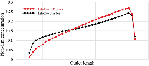
In Figure 21, the concentration profiles at the outlet of the tunnels with the elbow and tee downstream of the mixing section are compared. It is seen that the case with an elbow has a more non-uniform concentration profile. The average deviation from the mean value, not including the wall values, is 20% for the case with a Tee and 33% for the case with an elbow. The dilution tunnel with the tee provides a more uniform profile. As mentioned before, a dilution tunnel should have good mixing and a more uniform concentration at the outlet. Figure 21 proves that replacing the right elbow with a tee makes the concentration at the outflow more uniform.

Figure 21. Comparison of particle concentration profiles at the tunnel outlet for the Lab-2 tunnels with elbow and tee. Red dots present the Lab-2 tunnel with two elbows (case 1), and the black line represents the Lab-2 tunnel with elbow and tee (case 2).

Summary and conclusion

Particle concentration in turbulent flows in the dilution tunnels compliant with US EPA test methods was studied. The simulation results suggest that the Lab-1 tunnel with two tee joints generally provides more uniform concentrations at the test section. The Lab-2 dilution tunnel with 2 two-part elbows is simulated. It was found that under the normal operating conditions, when the stack flow concentration is uniform, the concentration profile also becomes uniform. To provide insight into the occasionally observed non-uniform concentration at the test section of the Lab-2 dilution tunnel, additional simulations were performed. Attention was given to the Lab-2 tunnel with elbow and tee joints with the highly non-uniform concentration entering from stack flow. Simulations were performed for identical boundary conditions. The only difference between the two configurations was the connection of the dilution section and pipe after the mixing section, leading to the test section. This connection was an elbow for the first case, and for the second case, it was a tee. The simulation results showed that the Lab-2 dilution tunnel with elbows for the case that the high-velocity stack flow concentration is highly non-uniform leads to a non-uniform concentration profile at the tunnel outlet. When the second elbow is replaced with a tee, the nonuniformity at the test section is markedly reduced. Comparison of the outlet particle concentration profiles shows that the use of the tee joint provides a more uniform concentration compared to the case that the elbow is used. This finding indicates that using a single tee increases the turbulence intensity, provides better mixing, and enhances the performance of dilution tunnels. For the tunnel designs specified by both ASTM-E2515 and EPA Method 5 G, the drawings label both turns as elbows and show the turns as smooth bends, not the 90-degree two-part elbows, as shown in Figure 7. However, other than using the term “elbow,” the method text is silent on this tunnel design element and does not explicitly state if two-part elbows or tees can also be used. This analysis shows that if mixing is a concern, the additional turbulence from the use of tees instead of two-part elbows can enhance mixing. The use of smooth elbows, as shown in the dilution tunnel method drawings, was not evaluated.

There are some limitations to this analysis. First, input parameters to the models such as stack flow and temperature use approximate values and assume steady-state conditions. However, these parameters can vary rapidly and widely during a multi-hour test run. Second, only 2D simulations were performed. Third, it is assumed that the stack is precisely centered under the hood when it may not have been. Fourth, while the potential for the spatial nonuniformity of the particle concentrations coming out of the woodstove stack is included in these simulations, the transient variation of concentration was not considered, which may be significant. These limitations may explain the differences between the well-mixed model output at normal stack flows and observations of transient poor mixing events.

Future studies are to consider the transient variations of stack flow, temperature, and concentration and fully 3D simulations of the dilution tunnels. In addition, assessing the influence of misalignment of the stack and hood on generating nonuniformity is part of future studies.

Data availability

The data that support the findings of this study are available from the corresponding author upon reasonable request.

Acknowledgment

The financial support of the New York State Energy Research Development Authority under contract #164575 to NESCAUM, Dr. Ellen Burkhard, Project manager, is gratefully acknowledged.

Disclosure statement

No potential conflict of interest was reported by the author(s).

Additional information

Funding

This work was supported by the New York State Energy Research and Development Authority [NYSERDA Agreement #164575].

Notes on contributors

Farid Rousta

Farid Rousta is a PhD student of Mechanical and Aeronautical Engineering at Clarkson University.

Goodarz Ahmadi

Goodarz Ahmadi is a Clarkson Distinguished Professor and Robert R. Hill Professor of Mechanical and Aeronautical Engineering at Clarkson University.

George Allen

George Allen is the Chief Scientist at NESCAUM.

References

- Allen, G., B. Morin, M. Ahmadi, and L. Rector. 2022. Online measurement of PM from residential wood heaters in a dilution tunnel. J. Air Waste Manage. Assoc.
- ASTM E2515-11. 2017. Standard test method for determination of particulate matter emissions collected by a dilution tunnel. West Conshohocken, PA: ASTM International. doi:10.1520/E2515-11R17.
- Birol, F. 2010. World energy outlook. Int. Energy Agency 1. https://scholar.google.com/scholar_lookup?title=World%20energy%20outlook%202010&publication_year=2010&author=F%20Birol
- Boman, C., A. Nordin, R. Westerholm, and E. Pettersson. 2005. Evaluation of a constant volume sampling setup for residential biomass fired appliances—influence of dilution conditions on particulate and PAH emissions. Biomass Bioenergy 29 (4):258–68. doi:10.1016/j.biombioe.2005.03.003.
- Breuer, M., H. Tarik Baytekin, and E. A. Matida. 2006. Prediction of aerosol deposition in 90∘ bends using LES and an efficient Lagrangian tracking method. J. Aerosol Sci. 37 (11):1407–28.
- Brockmann, J. E. 2001. Sampling and transport of aerosols. Aerosol Meas. 2:143–95.
- Cong, X. C., G. S. Yang, J. H. Qu, J. J. Zhao, et al. 2017. A model for evaluating the particle penetration efficiency in a ninety-degree Bend with a circular-cross section in laminar and turbulent flow regions. Powder Technol. 305:771–81. doi:10.1016/j.powtec.2016.10.074.
- Eilenberg, S. R., K. R. Bilsback, M. Johnson, J. K. Kodros, E. M. Lipsky, A. Naluwagga, K. M. Fedak, M. Benka-Coker, B. Reynolds, J. Peel, et al. 2018. Field measurements of solid-fuel cookstove emissions from uncontrolled cooking in China, Honduras, Uganda, and India. Atmos. Environ. 190:, 116–125. doi:10.1016/j.atmosenv.2018.06.041.
- Habibi, K. 1970. Characterization of particulate lead in vehicle exhaust-experimental techniques. Environ. Sci. Technol. 4 (3):239–48. doi:10.1021/es60038a001.
- He, C., and G. Ahmadi. 1999. Particle deposition in a nearly developed turbulent duct flow with electrophoresis. Journal of Aerosol Science 30 (6):813–31. doi:10.1016/S0021-8502(98)00760-5.
- Mofakham, A. A., and G. Ahmadi. 2019. Particles dispersion and deposition in inhomogeneous turbulent flows using continuous random walk models. Phys. Fluids 31 (8):083301–13. doi:10.1063/1.5095629.
- Mofakham, A. A., and G. Ahmadi. 2020. On random walk models for simulation of particle-laden turbulent flows. Int. J. Multiphase Flow 122:103157. doi:10.1016/j.ijmultiphaseflow.2019.103157.
- Obaidullah, M., B. Svend, and D. R. Jacques. 2018. Investigation of optimal dilution ratio from a dilution tunnel using in particulate matter measurement. Int. J. Eng. Sci. Technol. 5 (1):17–33. doi:10.15282/ijets.v5i1.2802.
- Ochieng, C. A., C. Tonne, and S. Vardoulakis. 2013. A comparison of fuel use between a low cost, improved wood stove and traditional three-stone stove in rural Kenya. Biomass Bioenergy 58:258–66. doi:10.1016/j.biombioe.2013.07.017.
- Peters, T. M., and D. Leith. 2004. Particle deposition in industrial duct bends. Ann. Occup. Hyg. 48 (5):483–90.
- Pui, D. Y. H., F. Romay-Novas, and B. Y. H. Liu. 1987. Experimental study of particle deposition in bends of circular cross section. Aerosol Sci. Technol. 7 (3):301–15. doi:10.1080/02786828708959166.
- Quek, T. Y., C.-H. Wang, and M. B. Ray. 2005. Dilute gas− solid flows in horizontal and vertical bends. Ind. Eng. Chem. Res. 44 (7):2301–15. doi:10.1021/ie040123i.
- Sevault, A., R. A. Khalil, B. C. Enger, Ø. Skreiberg, F. Goile, L. Wang, M. Seljeskog, and R. Kempegowda. 2017. Performance evaluation of a modern wood stove using charcoal. Energy Procedia 142:192–97. doi:10.1016/j.egypro.2017.12.031.
- Sun, K., L. Lu, H. Jiang, H. Jin, et al. 2013. Experimental study of solid particle deposition in 90 ventilated bends of rectangular cross section with turbulent flow. Aerosol Sci. Technol. 47 (2):115–24. doi:10.1080/02786826.2012.731094.
- Tian, L., and G. Ahmadi. 2007. Particle deposition in turbulent duct flows - Comparisons of different model predictions. Journal of Aerosol Science 38 (4):377–97. doi:10.1016/j.jaerosci.2006.12.003.
- Tissari, J., K. Hytönen, J. Lyyränen, and J. Jokiniemi. 2007. A novel field measurement method for determining fine particle and gas emissions from residential wood combustion. Atmos. Environ. 41 (37):8330–44. doi:10.1016/j.atmosenv.2007.06.018.
- Tsai, C.-J., and D. Y. H. Pui. 1990. Numerical study of particle deposition in bends of a circular cross-section-laminar flow regime. Aerosol Sci. Technol. 12 (4):813–31. doi:10.1080/02786829008959395.
- US Environmental Protection Agency. 2000. Method 5G determination of particulate matter emissions from wood heaters (dilution tunnel sampling location). Fed. Regist. 65 (201):61867–76.
- Walters, K., and D. Cokljat. 2008. A three-equation eddy-viscosity model for reynolds-averaged navier–stokes simulations of transitional flow. Journal of Fluids Engineering 130 (12):121401-1-14. doi:10.1115/1.2979230.
- Wilson, S. R., Y. Liu, E. A. Matida, M. R. Johnson, et al. 2011. Aerosol deposition measurements as a function of Reynolds number for turbulent flow in a ninety-degree pipe Bend. Aerosol Sci. Technol. 45 (3):364–75. doi:10.1080/02786826.2010.538092.