Observational-based assessment of contributions to maximum ozone concentrations in the western United States

ABSTRACT

Archived Ozone Design Values (ODVs) provide smoothed temporal records of maximum ozone concentrations impacting monitoring sites throughout the US. Utilizing time series of ODVs recorded at sites along the US West Coast, we separately estimate ODV contributions from US background ozone and from production driven by US anthropogenic precursor emissions. Sondes launched from Trinidad Head in northern California measure the vertical distribution of baseline ozone transported ashore from the Pacific; this profile is reflected in the increase of the US background ODV contribution with monitoring site elevation in both rural and urban areas. The ODVs that would result from US background ozone alone are small at coastal, sea level locations (average ~45 ppb), but increase with altitude; above 1 km US background ODVs can exceed 60 ppb. US background ozone contributions now constitute the majority of the maximum ODVs throughout the US west coast region, including the Los Angeles urban area, which records the country’s highest ODVs. US anthropogenic emissions presently cause enhancements of 35 to 55 ppb to the maximum ODVs in the Los Angeles area; thus, local emission controls can further reduce ozone even though the background contribution is larger. In other US west coast urban areas ODV enhancements from US anthropogenic emissions are much smaller than the US background ODV contribution. The past decrease in US anthropogenic ODV enhancements from emission controls is larger than generally realized – a factor of more than 6 from 1980 to 2020, while US background ODV contributions varied to only a small extent over those four decades. Wildfire impacts on ODVs are significant in urban areas of the Pacific Northwest, but not over the vast northern US rural region. There is an indication that agricultural emissions of nitrogen oxides in California’s Salinas Valley increase downwind maximum ODVs by 5–10 ppb.

Implications: In 2020 the ozone design values (ODVs) resulting from transported background ozone alone are now larger than the ODV enhancements from US anthropogenic precursor emissions, even in the Los Angeles urban area, where the nation’s highest ODVs are recorded. The US anthropogenic ODV enhancements have been reduced by more than a factor of 6 from 1980 to 2020. The maximum US background ODV contributions have varied somewhat, but in each of the US west coast urban areas it was 60 ppb or larger in 2000. These contributions are so large that reducing maximum urban ODVs to the 70 ppb required by the 2015 ozone NAAQS is very difficult. There remains relatively little room for further reducing ODVs through domestic emission controls alone. From this perspective, degraded US ozone air quality in the western US is primarily due to the US background ozone contribution, with the US anthropogenic enhancement making a significant, but smaller contribution. Notably, the US background ODV has slowly decreased (~1 ppb decade⁻¹; Parrish, Derwent, and Faloona 2021) since the mid-2000s; cooperative, international emission control efforts aimed at continuing or even accelerating this background ozone decrease may be an effective approach to further ODV reductions, since the US background ODV is largely due to a hemisphere-wide, transported reservoir of ozone with contributions from all northern midlatitude continents. Given the major contribution of background ozone to observed ODVs, future reviews of the ozone NAAQS will be better informed if observational-based estimates of background ODV contributions are considered, in addition to model-derived estimates upon which past reviews have solely relied.

Introduction

Since at least the 1940s, elevated ozone concentrations have degraded air quality in urban areas of the United States (Haagen-Smit 1954; National Research Council, 1991). Through extensive reductions of anthropogenic emissions of photochemical ozone precursors, great improvement has been made, but several areas of the country still exceed the 2015 National Ambient Air Quality Standard (NAAQS) for ozone (see US EPA Green Book 8-h Ozone 2015 Area Information; last accessed 11 July 2021). The NAAQS requires that the Ozone Design Value (ODV) not exceed 70 parts-per-billion (ppb, defined as nmole ozone/mole air). The ODV is defined as the 3-year running mean of the annual fourth-highest maximum daily 8-h average (MDA8) ozone concentration; it thus represents ~98^th percentile of MDA8 values observed in the warm half of the year, when those four highest values generally occur. A time series of ODVs observed at a particular monitoring station is thus a smoothed measure of the temporal evolution of the maximum ozone concentrations that impact that location. This work focuses on ODV time series recorded in the west coastal region of the US.

Early measurements of baseline ozone concentrations on the northwestern US coast (e.g., Singh, Ludwig, and Johnson 1978) show that air transported ashore from the Pacific marine environment carried ozone concentrations varying from about 20 to 60 ppb. At that time, these concentrations represented only a small fraction of maximum observed 1-hr average urban ozone concentrations, which exceeded 500 ppb in the mid-1960s in Los Angeles (Parrish and Stockwell 2015). Nevertheless, these transported concentrations can constitute a large fraction of the current NAAQS; thus, accurate estimates of the contribution of baseline ozone to ODVs are critical for informing US air quality policies. Baseline ozone is defined here as the ozone concentration in air transported to a location without recent local anthropogenic or continental influence [e.g., see discussion in Chapter 1 of HTAP (2010)]. For our purposes in this paper, this is air transported to a measurement location without significant perturbation of the marine ozone concentrations by continental influences.

A conceptual model is important for understanding US ambient ozone contributions from both scientific and air quality policy perspectives. First, it is important to recognize that both urban and rural ozone concentrations have important contributions from both natural and anthropogenic sources. Anthropogenic sources include local and regional photochemical production from US anthropogenic precursor emissions, as well as transport from more distant, potentially hemisphere-wide anthropogenic emissions. Natural sources include input from the stratosphere and photochemical production from natural precursor emissions such as oxides of nitrogen (NO_X) from lightning and soils, biogenic volatile organic carbon species (VOCs) from vegetation, and methane. Importantly, ambiguities arise because sources generally classified as natural may also have anthropogenic contributions, such as those associated with agriculture (soil NO_X emissions and methane), land use (biogenic VOCs), and oil and gas development (methane). In this work we view each ODV recorded at a particular site as having two distinct contributions: the first is the natural and anthropogenic ozone transported from outside the country, plus any ozone produced within the US from naturally emitted precursors – we refer to this contribution as the “US background ODV” – and the second is the enhancement of the recorded ODV above the US background ODV, which is due to photochemical production from US anthropogenic emissions of ozone precursors – we refer to this contribution as the “US anthropogenic ODV enhancement.” In the absence of US anthropogenic emissions, the US anthropogenic ODV enhancement would be zero, and the recorded ODV would simply be the US background ODV. These definitions are consistent with EPA’s definition of background ozone, referred to as US background ozone, which is designed to represent the influence of all sources other than US anthropogenic emissions (e.g., Dolwick et al. 2015). Section S4 of the Supporting Information presents an example analysis, based on synthetic data, that illustrates the significance of these two distinct ODV contributions. The text box below collects the important terms from above with their definitions; parameters introduced later are also included.

Table

Important quantitative terms and parameters with definitions MDA8 – Maximum daily 8-h average ozone concentration at a site on a particular day. Ozone Design Value (ODV) – 3-year running mean of the annual fourth-highest MDA8 ozone concentration at a site. US background ozone – The ozone concentration that would exist at a time and US location from all sources, except that produced from US anthropogenic emissions. Baseline ozone – The ozone concentration measured in air transported to a location without recent local or regional anthropogenic or continental influences. US background ODV – The ODV that would be recorded at a site in the absence of any contribution from US anthropogenic emissions. US anthropogenic ODV enhancement – The enhancement of an actual ODV above the US background ODV due to contributions from US anthropogenic emissions. a – Fit parameter of equation 3(3) $\mathrm{O}\mathrm{D}\mathrm{V}=a+0.20\ast \mathrm{t}-0.018\ast {\mathrm{t}}^2+A\mathrm{e}\mathrm{x}\mathrm{p}(-\mathrm{t}/\tau )$(3) that estimates the US background ODV in year 2000. A – Fit parameter of equation 3 that estimates the US anthropogenic ODV in year 2000. τ – Fit parameter of equation 3 that estimates the exponential rate of decrease of US anthropogenic ODV enhancement with time.

The categorization of ozone contributions from wildfires is somewhat ambiguous within this conceptual model. Wildfires have both natural and anthropogenic origins, and due to anthropogenic caused climate change, the wildfire ozone contributions that could possibly be classified as anthropogenic are believed to be increasing (e.g., Westerling 2016; Westerling et al. 2006). Notably, our analysis does not include any wildfire ozone contributions in the anthropogenic category, thus implicitly considering them to be natural. The ozone and precursors from wildfires can originate within the US or be transported from other countries. In this analysis, all wildfire contributions to an ODV are included in the US background ODV.

Formulation of ozone air quality control policies within the US has relied exclusively on photochemical grid models to provide estimates of US background ODVs (e.g., Dolwick et al. 2015), but those estimates have large uncertainties. An assessment of US background ozone determinations (Jaffe et al. 2018) estimate the uncertainty in modeled seasonal mean US background ozone as about ±10 ppb, with greater uncertainty for individual days. Since estimating the US background ODV at a particular site requires quantification of the background ozone concentrations on the individual days when the maximum MDA8 ozone concentrations were observed, the uncertainty associated with model-derived estimates of the background contribution to a specific ODV is likely greater than ±10 ppb. Another study (Guo et al. 2018) found even larger model biases of 0–19 ppb in seasonal mean MDA8 ozone; these were highest in summer, and the highest ozone events were simulated too late in the season. Thunis et al. (2021) evaluate source apportionment techniques that have been implemented within photochemical grid models, and find that they can underestimate local contributions compared that of the background. The presence of large model uncertainty is supported by comparisons of ODVs between different model simulations and between model- and observational-derived estimates. Parrish et al. (2017) show that six different model simulations gave US background ODV estimates for southern California that spanned the range from about 45 to 65 ppb, with a seventh simulation giving an outlier value of ~92 ppb; these model results can be compared to their observational-based result of 62 ± 2 ppb. Also, Parrish and Ennis (2019) show that three different model simulations gave US background ODV estimates that averaged 5 to 13 ppb lower than observational-based estimates at 4 locations across the northern US.

Comparison of model estimates with independent, observational-based estimates provides an approach to reduce the uncertainty of US background ODV quantification. Parrish et al. (2017) and Parrish and Ennis (2019) developed and utilized an observational-based analysis approach, which we apply here to separately quantify the US background ODV and the US anthropogenic ODV enhancement. This analysis is based on the very different temporal evolution of the two ODV contributions. Decreases of US anthropogenic ODV enhancements have been large and rapid; for example in the South Coast Air Basin (SoCAB), which contains the Los Angeles urban area, the maximum US anthropogenic ODV enhancements decreased by a factor of ~5 (i.e., from ~200 to ~40 ppb) at an approximately exponential rate from 1980 to 2015 (Parrish et al. 2017). This reduction has been driven by large decreases in anthropogenic precursor emissions; e.g., from 1960 to 2010 in the Los Angeles urban area, ambient concentrations of the two most important classes of anthropogenic ozone precursors, VOCs and NO_X, were reduced by factors of ~50 (Warneke et al. 2012) and ~4 (Pollack et al. 2013), respectively. In contrast, the US background ODVs, which can be considered to be due to the baseline ozone transported into the US, augmented by natural sources within North America, are expected to have changed relatively little. Baseline ozone concentrations have exhibited only small (a few ppb) systematic changes (Parrish, Derwent, and Faloona 2021) over recent decades, and natural ozone sources over North America are also not expected to have changed markedly. The very different temporal behaviors of the two ODV contributions allow us to estimate each component separately.

The observational-based approach applied here also has uncertainties. A fundamental assumption is that the ODV contributions from all US anthropogenic sources have decreased together over the past three to four decades. Without additional analysis, any anthropogenic ozone contribution that has not decreased would be interpreted as part of the US background ODV, rather than properly identified as a contribution to the US anthropogenic ODV enhancement. Two such confounding situations have been identified in previous work. Parrish et al. (2017) found a US background ODV in the Salton Sea Air Basin that was ~12 ppb larger than those in nearby air basins; a suggested cause of this difference is ozone contributions from large precursor emissions from the intense agricultural activities in the Imperial Valley (located in the Salton Sea Air Basin). Parrish and Ennis (2019) noted that recently recorded ODVs in the most densely populated areas of the northeastern US (i.e., New York City urban area) are a few ppb larger than the sum of the US background ODV plus the US anthropogenic ODV enhancement expected for that area based on results for the entire region. This disagreement has been tentatively attributed to ozone contributions from volatile chemical products (VCPs; McDonald et al. 2018), which are concentrated in densely populated areas. Precursor emissions from agricultural activities and VCP sources have not been controlled, at least to the same extent as other emission sectors, giving rise to these uncertainties. Importantly, biases arising from these uncertainties are relatively small, and examination of the spatial and temporal distributions of the derived ODV contributions can identify such uncertainties in the observational-based approach as discussed in Section 5.2.

The goal of this work is two-fold. We apply our observational-based approach to the west coastal region of the US, including the Pacific coastal air basins of southern California (CA), portions of northern CA, and the entire states of Oregon (OR), Washington (WA) and Idaho (ID). It is in this coastal region that we expect to most easily distinguish the US anthropogenic contribution from that of baseline ozone and other contributions to the US background ODV. Our first goal is to improve our scientific understanding of the contribution that US background ozone makes to maximum ozone concentrations observed in this region. Our second goal is to provide improved guidance for US air quality policy formulation. In this regard, additional analysis is included of ODVs recorded further inland in Montana, North Dakota and South Dakota. The recent 2020 policy assessment of the ozone NAAQS (US EPA 2020a, 2020b) did not consider the available observational-based quantifications of the US background ODVs, instead relying solely on model-derived estimates. We aim to expand the breadth of observational-based analyses so that future assessments can have a more robust scientific foundation, which is critical to setting NAAQS that not only maximize human health protection, but also are achievable through practical emission control strategies. In the following, Section 2 introduces the data sets analyzed and Section 3 discusses the analysis approach that allows separate quantification of the US background ODV and the US anthropogenic ODV enhancement. Section 4 describes the analysis results, which quantify the spatial variation of these two ODV contributions throughout this coastal region; Section 5 discusses the results and presents conclusions.

Data sets analyzed

This work examines ODVs reported from the beginning of US ozone monitoring in the mid-1970s through 2020 at coastal and nearby inland locations in California, and in the states of Oregon, Washington, Idaho, Montana and North and South Dakota. The ODVs are computed and published annually on EPA’s AQS data archive (https://www.epa.gov/aqs; last accessed 11 October 2021) by EPA’s Office of Air Quality Planning and Standards. A value is calculated each year for each ozone monitoring station in the US, if the measurements achieve the specified completeness criteria. The ODVs reported for all years at all sites in the regions of interest were downloaded from this archive; only the ODVs marked as valid were retained for analysis. The California Air Resources Board maintains a separate archive of ODVs (https://www.arb.ca.gov/adam/index.html; last accessed 7 July 2021), which contains ODVs from some sites not reported to EPA’s AQS data archive; we have included sites from this archive to supplement the primary set of ODVs. It should be noted that very few if any sites have continuous measurements over the full monitoring period, and that many sites operated for only short time periods. Generally, all reported ODVs are included in this analysis, even if only a single ODV was reported for a particular site. It is implicitly assumed that the temporal discontinuities associated with initiation or termination of individual sites do not prevent an accurate quantification of temporal trends of ODVs within the regions selected for analysis.

Networks of ozone monitoring sites have operated in the largest coastal urban areas in the region of focus – Los Angeles, San Francisco and Seattle; the ODVs from these networks are examined in detail. Rural regions and smaller urban areas are much less extensively sampled, but ODVs recorded at these sites provide valuable comparisons and contrasts to the three large urban centers.

We use the tabulated ODVs for two purposes – quantification of maximum ozone concentrations impacting surface locations, and as an indication of whether a particular measurement site is approaching or exceeding the NAAQS. There are air quality policy considerations that could potentially bias the applications of archived ODVs for these purposes. If the EPA concurs that certain data are influenced by exceptional events, such as wildfires or stratospheric ozone intrusions, and therefore not subject to comparison with the NAAQS, then the ODVs in EPA’s AQS data archive are changed from the value directly derived from the observational data. (More details of the Exceptional Events Rule can be found on the US EPA website: https://www.epa.gov/air-quality-analysis/treatment-air-quality-data-influenced-exceptional-events-homepage-exceptional). Thus, any ODVs that have been reduced through exceptional event concurrence from the US EPA are included in our analysis, and our ODV comparisons to the NAAQS are unaffected. However, if the EPA were to concur with a significant number of exceptional events, then the tabulated ODVs would underestimate the maximum ozone concentrations at any site affected by EPA’s concurrences. Fortunately for our purposes, such EPA concurrences have been rare. As far as we can determine through contact with state officials and an internet search, since the implementation of the 2016 Exceptional Events Rule EPA has not concurred with any exceptional event demonstrations in the region considered in this study. However, it should be noted that ODVs can be reduced, not only by precursor emission reductions, but also by EPA exceptional event concurrences, but to date no concurrence has been made that affects our analysis.

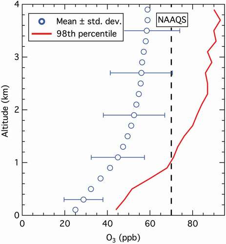
The Global Monitoring Laboratory of NOAA has measured vertical profiles of ozone with balloon-borne sondes launched from Trinidad Head on the northern California coast since 1997 (Oltmans et al. 2008; Sterling et al. 2018), generally on a weekly basis. This location is indicated in a later figure. Here, we consider the 533 sondes launched from 1997 to 2017 during the months of May through September (data available from https://esrl.noaa.gov/gmd/dv/data/index.php?category=Ozone&site=THD; last accessed 3 April 2018). Means with standard deviations and 98^th percentile values for 200 m altitude intervals of the combined data set are derived; Figure 1 shows these results.

Figure 1. Vertical profile of ozone mixing ratios measured by sondes launched from Trinidad Head CA (located on the northern California coast) from May through September, 1997–2017. Means with standard deviations and 98th percentiles are plotted for 200 m altitude increments.

Quantification of long-term O₃ changes

Our analysis is based on the quantification of long-term (i.e., time periods of a decade or more) changes in time series of tabulated ODVs from the many ozone measurement sites near the US west coast. Since ODVs are based on the fourth highest MDA8 ozone concentration in a given year, ODV time series have no variation on periods shorter than 1 year, but there are sources of ozone variability (i.e., sub-decadal interannual variability, or intense short-term events such as wildfires or stratospheric intrusions) that can obscure the systematic, long-term changes on which we focus. Our approach is to fit a continuous functional form to an ODV time series in order to objectively quantify the average long-term changes, even in the presence of significant, shorter-term variability. The parameter values derived from the fits are then interpreted to quantify the US background ODV and the US anthropogenic ODV enhancement for that particular time series.

ODVs recorded in major US urban areas have decreased rapidly over the past decades. Parrish et al. (2017) used a simple functional form to quantify the long-term changes in the maximum ODVs recorded in southern California,

(1) $\mathrm{O}\mathrm{D}\mathrm{V}=y_0+A\mathrm{e}\mathrm{x}\mathrm{p}(-\mathrm{t}/\tau )$(1)

The physical picture underlying Equation 1(1) $\mathrm{O}\mathrm{D}\mathrm{V}=y_0+A\mathrm{e}\mathrm{x}\mathrm{p}(-\mathrm{t}/\tau )$(1) is the conceptual picture discussed in the introduction; a constant background contribution, y₀, represents the US background ODV, and an exponentially decreasing second term corresponds to the US anthropogenic ODV enhancement. The parameter A is the magnitude of US anthropogenic ODV in the year 2000, and τ is the time constant of the exponential decrease; t = year – 2000 is the time in years referenced to the year 2000. A fit of Equation 1(1) $\mathrm{O}\mathrm{D}\mathrm{V}=y_0+A\mathrm{e}\mathrm{x}\mathrm{p}(-\mathrm{t}/\tau )$(1) captured a large fraction of the ODV variability (r² = 0.984) in seven southern CA air basins over the 1980–2015 period (Parrish et al. 2017). Parrish and Ennis (2019) demonstrate that Equation 1(1) $\mathrm{O}\mathrm{D}\mathrm{V}=y_0+A\mathrm{e}\mathrm{x}\mathrm{p}(-\mathrm{t}/\tau )$(1) also quantifies the long-term changes of ODVs in the northeastern US over the shorter 2000–2017 period, and give an extended justification for the selection of this particular functional form.

Long-term changes of baseline ozone concentrations at northern midlatitudes have been the subject of many analyses; these documented changes can inform us regarding changes in the US background ODV, since these quantities are related. European baseline ozone data sets are most extensive; Logan et al. (2012) analyzed several of those data sets to show that ozone increased by 6.5–10 ppb in 1978–1989 and 2.5–4.5 ppb in the 1990s, with that increase ending and a maximum reached in the 2000s, followed by decreasing concentrations, at least in summer. Parrish et al. (2020) analyzed those same data sets, which by then extended through 2018, plus additional European and North American data sets; in total 8 baseline data sets from surface sites, sondes and aircraft over western Europe and western North America were considered. These measurements covered altitudes from sea level to 9 km. An important conclusion of this analysis is that, within statistical confidence limits, the same long-term baseline ozone change has occurred throughout northern midlatitudes at all altitudes from the surface through the mid-troposphere. Parrish, Derwent, and Faloona (2021) show that this common northern midlatitude, long-term baseline ozone concentration change is consistent with 28 linear trend analyses that have been reported for baseline representative data sets collected in the western US, the region that is our focus in this work. This quantification utilizes a quadratic polynomial fit to multiple data sets

(2) ${\mathrm{O}}_{3\mathrm{b}\mathrm{a}\mathrm{s}\mathrm{e}\mathrm{l}\mathrm{i}\mathrm{n}\mathrm{e}}=a+bt+c{t}^2$(2)

where b = 0.20 ± 0.06 ppb yr⁻¹ and c = −(18 ± 6) × 10⁻³ ppb yr⁻², and a varies with location, primarily determined by altitude. Baseline ozone increased from the beginning of measurements in the 1970s, with that rate of increase slowing until maximum concentrations were reached in the year 2005.7 ± 2.5, followed by a slow decrease. It should be noted the temporal variation given by Equation 2(2) ${\mathrm{O}}_{3\mathrm{b}\mathrm{a}\mathrm{s}\mathrm{e}\mathrm{l}\mathrm{i}\mathrm{n}\mathrm{e}}=a+bt+c{t}^2$(2) is small; since 1990 the standard deviation of the 14 2-year means over the 1990–2017 period is 1.5 ppb (Parrish et al. 2020); generally, ODV interannual variability is as large as this standard deviation of baseline ozone concentrations.

For the analysis in this paper, we use Equation 2(2) ${\mathrm{O}}_{3\mathrm{b}\mathrm{a}\mathrm{s}\mathrm{e}\mathrm{l}\mathrm{i}\mathrm{n}\mathrm{e}}=a+bt+c{t}^2$(2) to estimate a time-varying US background ODV to replace y₀, which modifies Equation 1(1) $\mathrm{O}\mathrm{D}\mathrm{V}=y_0+A\mathrm{e}\mathrm{x}\mathrm{p}(-\mathrm{t}/\tau )$(1) to give Equation 3(3) $\mathrm{O}\mathrm{D}\mathrm{V}=a+0.20\ast \mathrm{t}-0.018\ast {\mathrm{t}}^2+A\mathrm{e}\mathrm{x}\mathrm{p}(-\mathrm{t}/\tau )$(3) :

(3) $\mathrm{O}\mathrm{D}\mathrm{V}=a+0.20\ast \mathrm{t}-0.018\ast {\mathrm{t}}^2+A\mathrm{e}\mathrm{x}\mathrm{p}(-\mathrm{t}/\tau )$(3)

Equation 3(3) $\mathrm{O}\mathrm{D}\mathrm{V}=a+0.20\ast \mathrm{t}-0.018\ast {\mathrm{t}}^2+A\mathrm{e}\mathrm{x}\mathrm{p}(-\mathrm{t}/\tau )$(3) explicitly equates the time dependence of the US background ODV with that of the transported baseline ozone concentrations. This is justified because the only other contribution to the US background ODV besides baseline ozone is natural ozone sources within the US, which are expected to have remained relatively constant. Equation 3(3) $\mathrm{O}\mathrm{D}\mathrm{V}=a+0.20\ast \mathrm{t}-0.018\ast {\mathrm{t}}^2+A\mathrm{e}\mathrm{x}\mathrm{p}(-\mathrm{t}/\tau )$(3) has three unknown parameters (a, A and τ), since values of b and c are taken from Parrish et al. (2020). The analysis presented in this paper is based on determining the three parameters in Equation 3(3) $\mathrm{O}\mathrm{D}\mathrm{V}=a+0.20\ast \mathrm{t}-0.018\ast {\mathrm{t}}^2+A\mathrm{e}\mathrm{x}\mathrm{p}(-\mathrm{t}/\tau )$(3) through least-squares regression fits of Equation 3(3) $\mathrm{O}\mathrm{D}\mathrm{V}=a+0.20\ast \mathrm{t}-0.018\ast {\mathrm{t}}^2+A\mathrm{e}\mathrm{x}\mathrm{p}(-\mathrm{t}/\tau )$(3) to time series of ODVs recorded within selected regions. Figure S1 illustrates example fits for different A parameter values, parameter a = 0, and τ = 21.8 years (value derived later in this analysis). Fits derived in analyses of actual ODV time series are positively offset by non-zero values of parameter a. Once these parameter values are derived from the fit of Equation 3(3) $\mathrm{O}\mathrm{D}\mathrm{V}=a+0.20\ast \mathrm{t}-0.018\ast {\mathrm{t}}^2+A\mathrm{e}\mathrm{x}\mathrm{p}(-\mathrm{t}/\tau )$(3) to an ODV time series, the time-dependent US background ODV and US anthropogenic ODV enhancement are given by the first three terms and the last term, respectively, of Equation 3(3) $\mathrm{O}\mathrm{D}\mathrm{V}=a+0.20\ast \mathrm{t}-0.018\ast {\mathrm{t}}^2+A\mathrm{e}\mathrm{x}\mathrm{p}(-\mathrm{t}/\tau )$(3) .

Quantified uncertainties of all derived parameter values are important in the following discussion; we consistently give 95% confidence limits, unless indicated otherwise. These confidence limits are derived from the least-squares routines utilized to fit the ODV time series to Equation 3(3) $\mathrm{O}\mathrm{D}\mathrm{V}=a+0.20\ast \mathrm{t}-0.018\ast {\mathrm{t}}^2+A\mathrm{e}\mathrm{x}\mathrm{p}(-\mathrm{t}/\tau )$(3) . Each ODV is a three-year running mean, so only every third ODV is independent from the others reported for a given site. Consequently, the number of independent ODVs in each fit is approximately a factor of three smaller than the number of reported ODVs, and the fitting routines therefore underestimate the true confidence limits of the derived parameters. To account for this autocorrelation in the ODV time series all reported confidence limits have been increased by a factor of 3^1/2. There likely are additional sources of covariance between the ODVs included in any particular fit. The ODVs from different sites within a region can co-vary due to regionally coherent interannual variability, and temporal interannual variability may possibly lead to covariance between ozone concentrations measured in successive years at a site. We are not able to account for the effect of this additional covariance; thus the derived confidence limits are lower limits for the true confidence limits of the derived parameters.

Results

As air masses come ashore from over the Pacific Ocean, the ozone vertical profile characteristic of the marine environment (cf. Figure 1) interacts with the convective boundary layer and coastal topography to begin mixing ozone through the lower levels of the troposphere. Section 4.1 quantifies the vertical profile of ozone concentrations transported ashore, and the following sections 1) investigate how that marine ozone distribution is modified by interactions with the continental environment to define the US background ODV, and 2) quantify the US anthropogenic ODV enhancement to produce the observed ODVs over the past 4 decades, within selected regions along the US west coast.

Vertical distribution of ozone in the Pacific marine environment

Ozone profiles measured by balloon-borne sondes released from Trinidad Head on the northern California coast allow quantification of the vertical distribution of baseline ozone concentrations transported ashore. Figure 1 shows results for the 535 vertical profiles measured in May through September from 1997 to 2017. Means with standard deviations and 98^th percentiles are shown; as noted in the Introduction, these 98^th percentiles are representative of the ODVs that would be recorded at a site at the corresponding altitude. Ozone varies significantly at all altitudes; below 4 km altitude standard deviations average 28% of the means, and the 98^th percentiles average 58% larger than the means.

Spatial distribution of ODV contributions in southern California air basins

Maximum ozone concentrations in southern California coastal urban areas reached very large enhancements by at least the 1950s, but have been substantially reduced over the past 4 to 5 decades, as shown in Figures 2, 3 and S2. The red curves in Figures 2 and 3 indicate a simultaneous fit of Equation 3(3) $\mathrm{O}\mathrm{D}\mathrm{V}=a+0.20\ast \mathrm{t}-0.018\ast {\mathrm{t}}^2+A\mathrm{e}\mathrm{x}\mathrm{p}(-\mathrm{t}/\tau )$(3) to the maximum ODVs from seven southern California air basins (Supplement Section S1 gives details). This fit allows precise determination of the value of the τ parameter = 21.8 ± 0.8 years, which provides an estimate for the e-folding time for the decrease in the US anthropogenic ODV enhancement. This value is used in the analyses of all ODV time series in this work.

Figure 2. (left) Topographical map showing locations of all sites in four southern California air basins reporting ODVs for 1975-2020. Violet diamonds are sites reporting air basin maximum ODVs and light blue circles indicate selected near-coastal sites. (right) Time series of ODVs recorded at sites in the South Coast Air Basin. Curves show fits to maximum ODVs (red squares and curve - see Table S1 for curve fit parameters), all ODVs (grey circles and black curve), and ODVs from the coastal sites (blue circles and curve).

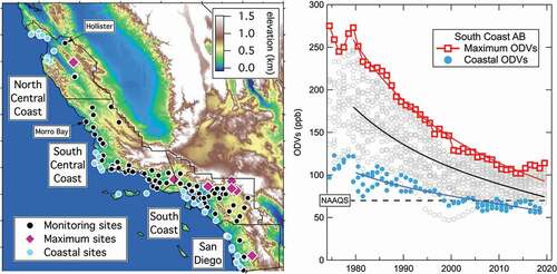
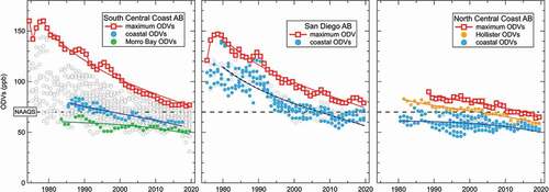
Figure 3. Time series of ODVs recorded at sites in three southern California air basins; note expanded y-axis range compared to Figure 2. Red squares and curves show maximum ODVs, and respective fits (see Table S1 for curve fit parameters). Blue circles and curves show results for coastal sites. Annotations identify symbols and fits for ODVs from two additional sites. Grey circles indicate ODVs from other sites.

Each of the coastal air basins contains many monitoring sites, some located near the Pacific Coast that have reported ODVs significantly smaller than the maximum ODVs analyzed in Section S1. Fitting Equation 3(3) $\mathrm{O}\mathrm{D}\mathrm{V}=a+0.20\ast \mathrm{t}-0.018\ast {\mathrm{t}}^2+A\mathrm{e}\mathrm{x}\mathrm{p}(-\mathrm{t}/\tau )$(3) to ODVs recorded at single sites or selected groups of sites allows an analysis of the broad features of the spatial distribution of the ODV contributions. Figures 2 and 3 include a total of eleven such fits in the four southern California air basins. Table S2 of the Supplement gives the derived parameter values, as well as other statistical details of the fits discussed in Sections 4.2–4.5; many of the parameter values in this table are also given in tables included in later figures. Table S3 lists the AQS site IDs for all ODVs included in those fits.

All four air basins in Figures 2 and 3 exhibit similarities in behavior. In each air basin, a set of selected near-coastal sites (blue symbols in map and graphs) record the smallest ODVs. In general, the widths of the ODV distributions in each air basin have decreased over time, with a tendency for all ODVs to converge toward the coastal ODVs. Table 1 compares the parameter values derived from ODV fits for coastal sites to those derived from the maximum ODVs. The A parameter values from the coastal sites are generally smaller by a factor of at least ~2 compared to the values from the maximum ODVs; one exception is the San Diego Air Basin, where the coastal A parameter value is only ~14% smaller than that for the maximum ODVs.

Table 1. Summary of spatial distribution of year 2000 maximum ODV contributions in four southern California air basins

Air Basin	a (ppb) ^1 coastal	A (ppb) ^1 coastal	a (ppb) ^2 maximum	A (ppb) ^2 maximum
South Coast	50 ± 6	26 ± 4	63 ± 1	82 ± 3
San Diego	47 ± 5	32 ± 3	“	37 ± 2
South Central Coast	50 ± 4	19 ± 3	“	40 ± 2
North Central Coast	50 ± 2	9 ± 2	“	17 ± 2

¹Parameter values derived from fits of Equation (3)(3) $\mathrm{O}\mathrm{D}\mathrm{V}=a+0.20\ast \mathrm{t}-0.018\ast {\mathrm{t}}^2+A\mathrm{e}\mathrm{x}\mathrm{p}(-\mathrm{t}/\tau )$(3) to ODVs recorded at selected coastal sites in respective air basins.

²Parameter values derived from the simultaneous fit of Equation (3)(3) $\mathrm{O}\mathrm{D}\mathrm{V}=a+0.20\ast \mathrm{t}-0.018\ast {\mathrm{t}}^2+A\mathrm{e}\mathrm{x}\mathrm{p}(-\mathrm{t}/\tau )$(3) to the maximum ODVs recorded in seven southern California air basins, as described in Section S1 of the Supplement.

ODVs recorded at sites inland from the coast (gray, red and gold symbols in Figures 2 and 3) generally are larger than those at the coastal sites, indicating increasing anthropogenic impact inland from coastal areas. For example, in the SoCAB the A parameter derived from the fit to all 1057 ODVs recorded at all sites from 1980 to 2020 is 54 ± 5 ppb, which is approximately two-thirds of the value derived from the fit to the maximum ODVs (82 ± 3 ppb) in the basin.

ODV contributions in rural northern California

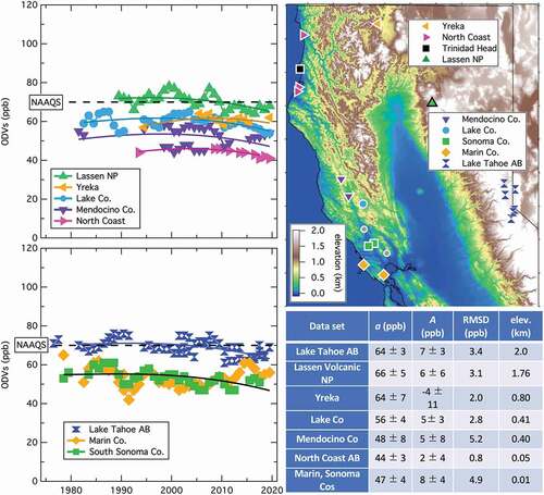
A number of monitoring sites have operated in the predominately rural region of California north of San Francisco (see map in Figure 4). The two graphs in Figure 4 show seven time series of ODVs recorded at single or multiple sites near the Pacific Coast and at more inland sites north of California’s urban areas. The Table in Figure 4 gives the parameter values derived from the fits of Equation 3(3) $\mathrm{O}\mathrm{D}\mathrm{V}=a+0.20\ast \mathrm{t}-0.018\ast {\mathrm{t}}^2+A\mathrm{e}\mathrm{x}\mathrm{p}(-\mathrm{t}/\tau )$(3) to those seven ODV time series. The derived A parameters (−4 to 8 ppb) indicate that US anthropogenic ODV enhancements are small at all of these rural sites; evidently observed ozone concentrations throughout this region are determined primarily by ozone transported ashore from the Pacific marine environment. Notably, larger a parameter values (i.e., US background ODV values) are derived from the fits to the ODV time series collected at higher elevations (see Table in Figure 4), consistent with the vertical gradient of baseline ozone concentrations, as shown in Figure 1.

Figure 4. Temporal evolution of ODVs recorded at single sites or groups of sites in rural northern California; note the expanded y-axis range in the graphs compared to those of Figures 2 and 3. The map shows site locations, with symbol colors and shapes identifying sites, which are the same in the graphs and the map. Curves indicate fits of Equation 3 with derived parameter values given in table. The location of the Trinidad Head ozone sonde launch site is also indicated.

Spatial distribution of ODV contributions in the San Francisco bay area air basin

The San Francisco Bay Area Air Basin (SFAB) includes the largest urban area in northern California, but the ODVs recorded here over the past 45 years have seldom exceeded 100 ppb. Figure 5 includes separate fits of Equation 3(3) $\mathrm{O}\mathrm{D}\mathrm{V}=a+0.20\ast \mathrm{t}-0.018\ast {\mathrm{t}}^2+A\mathrm{e}\mathrm{x}\mathrm{p}(-\mathrm{t}/\tau )$(3) to the time series of all recorded ODVs and to the maximum ODVs in SFAB. The US background ODVs derived from the all-site fit (a = 51 ± 3 ppb) agrees with the values derived from coastal locations throughout California, as expected for the near sea-level location of San Francisco. In contrast the fit to the maximum ODVs gives a significantly larger value for the a parameter (65 ± 5 ppb); importantly the A parameter value from this fit (i.e., the estimated maximum US anthropogenic ODV enhancement in 2000) is 19 ± 4 ppb in SFAB, much smaller than the 82 ± 3 ppb value derived in SoCAB. It is notable that 2020 was the first year that all ODVs reported for the SFAB were below the ozone NAAQS.

Figure 5. Temporal evolution of ODVs in the San Francisco Bay Area Air Basin; map shows locations of the sites. Symbol colors and shapes identify sites that record the maximum ODVs in the air basin and two sites showing evidence of reduced ozone due to ozone titration by fresh NO emissions. Curves indicate fits of Equation 3 with derived parameter values given in table.

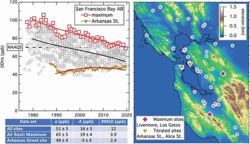
An interesting feature of the ODVs in SFAB is that, while the maximum and mean ODVs decrease over the measurement record, the smallest observed ODVs show a tendency to increase. The ODVs recorded at the Arkansas St. site (the most centrally located San Francisco site; Figure 5) were smaller than the estimated US background ODV for the area; similar behavior is seen at the most centrally located Oakland site (Alice Street Site), also indicated in the map.

Spatial distribution of ODV contributions in the Pacific Northwest

In the Pacific Northwest, we consider the ODVs recorded in three states (Figure 6); Seattle (Figure 7), another large US metropolitan area, is in this region. Generally, the entire region is characterized by lower ODVs than the regions further south. Only one ODV above 90 ppb has ever been recorded, and very few ODVs have exceeded the 70 ppb NAAQS during the past decade. Vast areas of this region (interior sites – green circles in Figure 6) are predominately rural; remarkably little variation is seen in the ODVs recorded at these sites, with only small US anthropogenic ODV contributions (A = 8 ± 4 ppb). The longest ODV time series in this rural region was collected in Medford OR, a small metropolitan area (population ~ 286,000 in 2010) near the California border that sits astride Interstate Highway 5. The US anthropogenic ODV enhancement in Medford (A = 9 ± 3 ppb) is similar to that of the entire region. These inland areas are at, or at least downwind of, higher elevation topography, and record higher US background ODVs (a = 62 ± 4 ppb and 60 ± 3 ppb for Medford and the entire region, respectively) than derived at coastal sites. Further north, Interstate Highway 5 passes through larger cites (Eugene, Salem and Portland – red diamond symbols), which lie at lower elevations; consequently, the fit to Equation 3(3) $\mathrm{O}\mathrm{D}\mathrm{V}=a+0.20\ast \mathrm{t}-0.018\ast {\mathrm{t}}^2+A\mathrm{e}\mathrm{x}\mathrm{p}(-\mathrm{t}/\tau )$(3) gives a slightly larger A parameter (13 ± 2 ppb), but a smaller a parameter (54 ± 3 ppb), compared to the interior sites.

Figure 6. Temporal evolution of ODVs in the three northwestern US states. Map shows locations of the ozone monitoring sites. Symbol colors and shapes identify two groups of sites, plus a single site. The parameters derived from fits of Equation 3 to those data sets are given in the table.

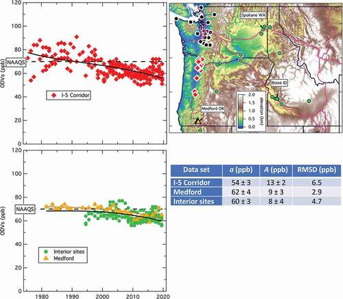
Figure 7. Temporal evolution of ODVs in northwest Washington, with map showing locations of the sites; the map is the expanded upper left portion of the map in Figure 6. Symbol colors and shapes identify two groups of sites, plus three single sites. For Seattle, each site that recorded the maximum ODV in any year is indicated in the map by a black outline. The parameters derived from fits of Equation 3 to three of those data sets are given in the table, along with averages with standard deviations (given as a values) of the limited ODV time series available from two of the single sites.

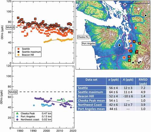
The fit to the ODVs at low elevation sites in the Seattle urban area (dark orange squares in Figure 7) gives a US anthropogenic ODV enhancement (A = 12 ± 3 ppb) and US background ODV (a = 56 ± 4 ppb) that are similar to those in the Interstate 5 corridor discussed above. In the group of sites on the northwest coast (purple diamonds in Figure 7) the fit gives a US anthropogenic ODV enhancement (A = 12 ± 7 ppb) that is similar to that in Seattle, but the US background ODV (a = 42 ± 6 ppb) is smaller than estimated for other coastal sites.

Only one site in Seattle shows significantly different behavior – the ODV time series at Beacon Hill (the most centrally located Seattle site – gold diamond in Figure 7). This time series behaves similarly to that of the Arkansas St. and Alice St. sites in SFAB, with a negative US anthropogenic ODV enhancement (A = −10 ± 6 ppb). The derived US background ODV at Beacon Hill (a = 52 ± 4 ppb) is consistent with that derived from the fit to all Seattle sites (56 ± 4 ppb). We attribute the behavior at these central urban sites to net destruction of US background ODVs by fresh NO emissions, particularly from vehicle emissions, which react with ozone and reduce ozone concentrations, including the ODVs, to below the baseline concentrations transported into the urban areas.

ODV variance

The ODVs considered in this work vary widely, from greater than 270 ppb in the SoCAB in 1980 (Figure 2) to ~40 ppb at both low elevation coastal sites and central urban sites in San Francisco and Seattle (Figures 4, 5 and 7). The fits of Equation 3(3) $\mathrm{O}\mathrm{D}\mathrm{V}=a+0.20\ast \mathrm{t}-0.018\ast {\mathrm{t}}^2+A\mathrm{e}\mathrm{x}\mathrm{p}(-\mathrm{t}/\tau )$(3) to the ODV time series capture a large fraction of this variability. The root-mean-square deviations (RMSDs) between the observed ODVs and the derived fits are given for each selected time series in annotations in Figures 4–7 and/or Table S2. The majority of these RMSDs are in the range of 2 to 5 ppb; exceptions are a larger RMSD (7.4 ppb) for the maximum ODV time series in SoCAB, and for time series that include a large number of sites in urban areas (fits to all sites in SoCAB, SFAB, the I-5 corridor and Seattle, and coastal sites in SoCAB and San Diego Air Basin). The cause of these larger RMSDs is attributed to spatial variability in the US anthropogenic ODV enhancement among the multiple sites included in these data sets. Overall, Sections S1 and S2 show that the fits of Equation 3(3) $\mathrm{O}\mathrm{D}\mathrm{V}=a+0.20\ast \mathrm{t}-0.018\ast {\mathrm{t}}^2+A\mathrm{e}\mathrm{x}\mathrm{p}(-\mathrm{t}/\tau )$(3) capture more than 97% of the variance of the maximum ODVs in seven southern California air basins, and 84% of the variance of the 22 ODV series discussed in Section S2. In later discussion, the small fractions of remaining variance are examined to provide additional information regarding processes contributing to variation of ODVs in these regions.

Discussion and conclusion

Long-term changes of US background ODVs have been very different from the long-term changes of US anthropogenic ODV enhancements within the country. Section 3 develops Equation 3(3) $\mathrm{O}\mathrm{D}\mathrm{V}=a+0.20\ast \mathrm{t}-0.018\ast {\mathrm{t}}^2+A\mathrm{e}\mathrm{x}\mathrm{p}(-\mathrm{t}/\tau )$(3) , which explicitly includes these different temporal changes; fits of this equation to time series of ODVs thereby provides separate estimates for these two contributions to recorded ODVs. Section 4 derives separate estimates for these two contributions in selected regions that encompass the entire US West Coast region. Here we discuss these results, provide additional investigation of the ODV variability, and discuss the implications for US air quality policy.

Systematic variability of ODV contributions in western US

Southern California coastal urban areas have consistently recorded the largest ozone concentrations in the US. The maximum ODVs recorded in four southern California air basins (Figures 2, 3 and S2) document the substantial reductions in these concentrations that have been accomplished over the past 4 to 5 decades. Importantly, the overall temporal changes of these maximum ODVs are much larger than the change of the baseline ozone concentrations; for comparison, the black curve in Figure S2 shows an estimate of the temporal evolution of maximum US background ODVs (the first three terms of Equation 3)(3) $\mathrm{O}\mathrm{D}\mathrm{V}=a+0.20\ast \mathrm{t}-0.018\ast {\mathrm{t}}^2+A\mathrm{e}\mathrm{x}\mathrm{p}(-\mathrm{t}/\tau )$(3) for southern California. A fit of Equation 3(3) $\mathrm{O}\mathrm{D}\mathrm{V}=a+0.20\ast \mathrm{t}-0.018\ast {\mathrm{t}}^2+A\mathrm{e}\mathrm{x}\mathrm{p}(-\mathrm{t}/\tau )$(3) to an ODV time series requires determination of three parameter values: a, A and τ. Only in southern California, where there have been such large temporal changes in ODVs, is it possible to derive precise values for all three parameters (see extensive discussion in Parrish et al. 2017). The red curves in Figures 2 and 3 (also included as colored curves in Figure S2) indicate a simultaneous fit of Equation 3(3) $\mathrm{O}\mathrm{D}\mathrm{V}=a+0.20\ast \mathrm{t}-0.018\ast {\mathrm{t}}^2+A\mathrm{e}\mathrm{x}\mathrm{p}(-\mathrm{t}/\tau )$(3) to the maximum ODVs from seven southern California air basins (Supplement Section S1 gives details of this fit). The parameter values derived for 1980–2020 are generally consistent with the results of Parrish et al. (2017), who fit shorter (1980–2015) time series. The τ parameter value derived in the present analysis (21.8 ± 0.8 years) provides an estimate for the e-folding time of the decrease in the US anthropogenic ODV enhancement. This value is used in the analysis of all ODV time series in this work; it agrees closely with the earlier estimate (21.9 ± 1.2 years) derived by both Parrish et al. (2017) for southern California, and used by Parrish and Ennis (2019) in their analyses of northeastern US ODVs.

The a parameter values derived from fits of Equation 3(3) $\mathrm{O}\mathrm{D}\mathrm{V}=a+0.20\ast \mathrm{t}-0.018\ast {\mathrm{t}}^2+A\mathrm{e}\mathrm{x}\mathrm{p}(-\mathrm{t}/\tau )$(3) to time series of ODVs from selected near-coastal, low elevation sites provide an estimate of the systematic spatial variability of the US background ODV near sea level along the entire US Pacific Coast. In the four southern California air basins (Figures 2 and 3), each fit to the five sets of coastal ODVs (including the single Morro Bay site, where a 37-year ODV time series has been collected at a location more removed from the southern California urban areas) gives an a parameter value that is consistent with their average of 49 ± 1 ppb. Values derived from fits to three time series collected at near-coastal sites (a = 46 ± 3 ppb) in northern California (Figure 4) are not significantly different from the southern California result. In northwest Oregon, two coastal data sets (Northwest Coast and Port Angeles, Figure 7) give somewhat smaller values (42 ± 6 ppb and 44 ± 1 ppb, respectively). These results demonstrate that the US background ODV near sea level has little spatial variability; this is expected, since these sites receive baseline ozone inflow from the marine boundary layer over the relatively uniform Pacific environment. Overall, the average a parameter value over the entire coast is about 45 ppb, with an indication of a small gradient, decreasing south (49 ± 1 ppb) to north (~43 ppb). This gradient is qualitatively consistent with earlier results, including modeled annual zonal mean ozone (c.f., Figure 2 of Crutzen, Lawrence, and Pöschl 1999) and median, near-surface US Pacific Coast ozone in May–June 2010 (Figure 5 of Cooper et al. 2011). The fits to all recorded ODVs in the SoCAB (Figure 2), SFAB (Figure 5) and Seattle (Figure 7) areas give a parameter values of (56 ± 6 ppb, 51 ± 3 ppb and 56 ± 4 ppb, respectively); these estimates are in accord with their near sea-level locations that also include sites at somewhat higher elevations.

Baseline ozone over the Pacific Ocean increases rapidly with altitude, particularly from the surface to above the marine boundary layer. Section 4.1 quantifies the marine ozone altitude profile (Figure 1) based on balloon-borne sonde measurements conducted at Trinidad Head on the northern California coast (location shown on map in Figure 4). Mean ozone mixing ratios are relatively small (~25 ppb) near the ocean surface, but increase rapidly with altitude, approaching ~60 ppb at 4 km. The 98^th percentiles shown in Figure 1 are approximately equivalent to ODVs, since an ODV is based on the fourth-highest daily MDA8, which corresponds to ~98^th percentile of the days in the photochemical ozone season. Notably, above an altitude of ~1 km the 98^th percentile exceeds 70 ppb, which corresponds to the NAAQS; thus a hypothetical inland surface site at 1 km or higher elevation that received only unperturbed marine air from that altitude would be expected to record ODVs exceeding the NAAQS due to transported baseline ozone alone.

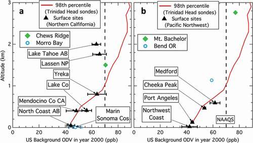
The altitude dependence of baseline ozone concentrations is reflected in the US background ODV values estimated by the a parameters derived in the fits to ODVs from surface sites at varying elevation. Figure 8a shows the dependence of US background ODVs on the elevation of the rural sites in northern California (Section 4.3), and compares that dependence to the 98^th percentile of marine ozone concentrations measured by the Trinidad Head sondes (Section 4.1). Also included in Figure 8a are the results from Morro Bay (Figure 3) and ODV estimates derived from ozone monitoring at Chews Ridge (Faloona et al. 2020), a baseline site in the coastal mountains south of San Francisco (Asher et al. 2018). Figure 8b shows the analogous plot for the Pacific Northwest, where similar dependence on site elevation is found. This figure includes the ODV estimates of Jaffe et al. (2018) for Bend OR and Mt. Bachelor, two rural Oregon sites. These US background ODV estimates approximately agree with those expected at the site elevations from the measured 98^th percentile marine ozone concentrations, at least up to ~1 km elevation. At higher elevations the US background ODVs are smaller than expected from transported marine air at that altitude. This difference may indicate that deposition to continental vegetation, combined with orographically forced vertical mixing, reduces ozone concentrations aloft as air moves inland from the Pacific coast. A similar process has been described for the gradual reduction of hemispheric baseline ozone mixing ratios during passage of air across the UK (Jenkin 2014).

Figure 8. Vertical profile of US background ODV estimates in year 2000 from surface sites in a) California (seven data sets from Figure 4 and Morro Bay from Figure 3) and b) the Pacific Northwest (four data sets from the lower graphs in Figures 6 and 7) compared to the 98th percentile of baseline ozone mixing ratios measured by Trinidad Head sondes (Figure 1). Black symbols are the a parameter values derived from the respective fits. Chews Ridge in a) and two sites in b) are from literature reports.

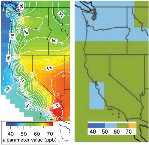
The contour map in Figure 9 gives a semi-quantitative representation of the spatial distribution of US background ODVs over the western US based on the a parameter values derived from the ODV time series fits summarized in Table S2, augmented by preliminary results from three additional southwestern US states. This map emphasizes the relatively small coastal values with increases inland in approximate agreement with the elevation of the underlying topography, as well as the decreasing south-to-north gradient along the coast.

Figure 9. Two estimates of the spatial variability of US background ODVs. (Left) Contour map developed from a parameter values determined in this work (with inclusion of preliminary results from ODV time series fits in Nevada, Arizona and Utah), augmented by extrapolation over the Pacific and into southern Canada. Symbols indicate individual monitoring sites included in the analysis with the same color coding. (Right) Annual 4th highest MDA8 ozone concentration averaged over 2010–2014, from a GFDL-AM3 model simulation with North American anthropogenic emissions zeroed out (figure reproduced from a section of Figure 3 of Jaffe et al. 2018).

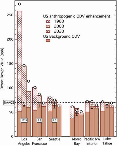
The derived US anthropogenic ODV enhancements, as quantified by the derived A parameter values, have a very different spatial distribution from that of the a values – the A parameter magnitudes are closely related to the urban population in or near the ODV measurement sites. For example, the SFAB (Figure 5) includes the largest urban area in northern California, but the ODVs recorded here over the past 45 years have seldom exceeded 100 ppb, much smaller than those recorded in the Los Angeles urban area, (> 270 ppb in 1980, Figure 2). These marked differences between the two largest California metropolitan areas reflect the different populations, emissions, meteorology and topography of the two cities. Figure 10 compares the ODV contributions derived from the maximum ODVs recorded in the three largest US west coast urban areas with those derived from the ODVs recorded in three rural areas. The populations of the urban areas (https://en.wikipedia.org/wiki/Combined_statistical_area) are annotated. A correlation between the US anthropogenic ODV enhancement and the urban population is clear. In the three rural areas, the A parameters are smaller than in the closest urban area, but are still significant, presumably due to ozone transport from nearby urban areas and/or ozone production from local and regional precursor emissions. Notably, the contrasting spatial distribution of the derived US background ODVs and the US anthropogenic ODV enhancements, support the conceptual picture that underlies our analysis.

Figure 10. Temporal evolution of ODVs recorded in six US West Coast areas over four decades. The bars indicate the US background ODV (solid area, showing the first 3 terms of Equation 3)(3) $\mathrm{O}\mathrm{D}\mathrm{V}=a+0.20\ast \mathrm{t}-0.018\ast {\mathrm{t}}^2+A\mathrm{e}\mathrm{x}\mathrm{p}(-\mathrm{t}/\tau )$(3) and the US anthropogenic ODV enhancement (hatched area, showing the exponential term of Equation 3)(3) $\mathrm{O}\mathrm{D}\mathrm{V}=a+0.20\ast \mathrm{t}-0.018\ast {\mathrm{t}}^2+A\mathrm{e}\mathrm{x}\mathrm{p}(-\mathrm{t}/\tau )$(3) in 1980, 2000 and 2020, as estimated from substitution of the respective fit parameters (Table S2) into Equation 3(3) $\mathrm{O}\mathrm{D}\mathrm{V}=a+0.20\ast \mathrm{t}-0.018\ast {\mathrm{t}}^2+A\mathrm{e}\mathrm{x}\mathrm{p}(-\mathrm{t}/\tau )$(3) . The three sets of bars on the left represent the maximum ODVs recorded in three major coastal urban areas (populations annotated in millions), and the three sets of bars on the right represent all ODVs recorded in three rural areas discussed in the text. The circles indicate the actual ODVs recorded in the respective years in each area or site. The error bars indicate the confidence limits of the a parameter values (Table S2), which are the estimated US background ODVs in the year 2000.

Biases in derived US background ODVs

The analysis in this paper is based on separately estimating the two ODV contributions based upon their very different temporal dependence; this is an indirect analysis, and potential systematic ambiguities remain in some of the derived estimates. Most importantly, in the 6 regions including the largest urban populations (SoCAB, San Diego, South Central Coast AB, North Central Coast AB, SFAB and the Seattle area) the a parameters derived from the maximum ODVs in each region are in the range of 60 to 65 ppb, while the values derived from fits to all of the ODVs in these same regions are in the range of 50 to 56 ppb. This difference implies that in each of these regions there are one or more sites that record ODVs that are consistently larger than those recorded at other sites in that region. Further, these ODV differences do not vary significantly over the ODV record. As a consequence fits of Equation 3(3) $\mathrm{O}\mathrm{D}\mathrm{V}=a+0.20\ast \mathrm{t}-0.018\ast {\mathrm{t}}^2+A\mathrm{e}\mathrm{x}\mathrm{p}(-\mathrm{t}/\tau )$(3) to the time series of maximum ODVs give larger a parameter values, compared to fits to the time series of all ODVs. Since similar US background ODV values are expected for all similar sites in a region, we interpret these systematically larger a values as due either to larger impacts from background ozone at those particular sites or to ODV contributions from precursor sources whose emissions have not been effectively controlled. Previous work suggested that three such emission sectors can cause such ODV biases – agricultural emissions (Parrish et al. 2017), wildfire emissions (Jaffe et al. 2020) and volatile chemical products (VCPs; Parrish and Ennis 2019). In this section we approximately quantify influences from agriculture and wildfires, and in Section S5 of the Supplement we present evidence indicating little influence from oil and gas production and other less well-controlled emissions in the western US region studied here.

In addition to potential systematic biases, there is chaotic variability in the ODV time series not captured by the analysis based on Equation 3(3) $\mathrm{O}\mathrm{D}\mathrm{V}=a+0.20\ast \mathrm{t}-0.018\ast {\mathrm{t}}^2+A\mathrm{e}\mathrm{x}\mathrm{p}(-\mathrm{t}/\tau )$(3) . As discussed in Section 4.6, the fits of Equation 3(3) $\mathrm{O}\mathrm{D}\mathrm{V}=a+0.20\ast \mathrm{t}-0.018\ast {\mathrm{t}}^2+A\mathrm{e}\mathrm{x}\mathrm{p}(-\mathrm{t}/\tau )$(3) to ODV time series do capture a large fraction of the ODV variance – more than 97% of the variance of the maximum ODVs in seven southern California air basins (Section S1), and 84% of the variance of the 22 ODV time series discussed in Section S2. The remaining variance (< 3% and 16%, respectively) are reflected in the RMSD deviations about the fits (generally 2 to 5 ppb as discussed in Section 4.6). This more chaotic, interannual variability is believed to arise from a variety of processes that have been shown to affect ambient ozone concentrations on a time scales of days to a few years; these processes include sporadic wildfire occurrence (Jaffe et al. 2008, 2020; McKeen et al. 2002; Pfister, Wiedinmyer, and Emmons 2008), stratospheric intrusions (Langford et al. 2015; Lin et al. 2012), and meteorological conditions that vary over sub-decadal time scales (Lin et al. 2015; Wang et al. 2016). Here we consider possible influences from these processes, with a particular focus on the impact of wildfire emissions.

Agricultural emissions, particularly NO_X emissions from fertilized crops (e.g., Almaraz et al. 2018) and agricultural equipment, can contribute to elevated ozone concentrations (e.g., Hall, Matson, and Roth 1996). Controls of such emissions have not been implemented over the past decades, certainly not as extensively as for other anthropogenic emissions. The Salton Sea Air Basin contains the Imperial Valley, one of the most intensely farmed regions of the country. The a parameter value estimated for this area (including Yuma AZ) is 70.5 ± 2.4 ppb (see detailed discussion in Supplement Section S3), which is significantly larger than for the other southern California air basins; the agricultural emissions in the Imperial Valley have been suggested (Parrish et al. 2017) as the cause of this large parameter value. In the North Central Coast air basin (Figure 3), the a parameter values derived from the time series of maximum ODVs (62 ± 4 ppb; all recorded at the Pinnacles NP site) and the ODVs from the Hollister site (56 ± 2 ppb) are 6 to 12 ppb (Table S2) larger than expected from their rural, relatively low elevation, near coastal locations and the fit to the ODVs recorded from other sites in the air basin (50 ± 2 ppb). This difference may reflect the influence of strong agricultural emissions biasing the derived a parameter values above the true US background ODV at these two sites, which are downwind of the Salinas Valley, an intensively farmed area where a large majority of the salad greens consumed in the U.S. are grown (https://en.wikipedia.org/wiki/Salinas_Valley). However, it should also be noted that Guo et al. (2020) find soils to be a small source of NO_X, and emission rates remain highly uncertain. Further investigation of the air quality impacts of agricultural activities in CA is recommended; we plan to undertake such work.

The northwestern US has been identified as a region of particularly strong air quality impacts from wildfire emissions (e.g., McClure and Jaffe 2018). The predominant impacts are elevated PM_2.5 concentrations, but elevated ozone concentrations have also been attributed to wildfire emissions (e.g., Buysse et al. 2019). These emissions have not decreased as have most anthropogenic emissions, so any wildfire impact on measured ODVs would be included in our estimate of the US background ODV. Rather than decreasing, Jaffe et al. (2020) find that wildfire frequency has increased; a significant impact from wildfire emissions would then cause an increasing trend in recorded ODVs. However, wildfire emissions are by their very nature sporadic in their temporal and spatial occurrence, which provides a means to identify their impact. Time series of ODVs recorded in the rural areas of the three Pacific Northwest states (OR, WA and ID) considered in this work, and in the three northern rural states (Montana and North and South Dakota) investigated by Parrish and Ennis (2019) that lie further inland, indicate that wildfire impacts on maximum ozone concentrations are not discernable in this vast rural region. This conclusion follows from two observations. First, the recorded ODVs exhibit remarkably little sporadic variability either in space or time; all ODVs recorded in this rural region covering six states over 40 years are well fit by Equation 3(3) $\mathrm{O}\mathrm{D}\mathrm{V}=a+0.20\ast \mathrm{t}-0.018\ast {\mathrm{t}}^2+A\mathrm{e}\mathrm{x}\mathrm{p}(-\mathrm{t}/\tau )$(3) with RMSDs of 1.3 to 4.3 ppb (see Figure S5), and the standard deviations of the means of the ODVs recorded at all sites throughout the measurement record in each of the three more easterly states (Montana and North and South Dakota) are 2.6 to 4.3 ppb. Second, the ODVs in this region are in general decreasing, not increasing as are estimated wildfire emissions. Detailed discussion of this analysis is given in Section S3 of the Supplement. A firm conclusion emerges – wildfires simply do not have a discernable impact on ODVs recorded throughout this rural northern US region.

In contrast to this rural region, significant wildfire impacts on the maximum ODVs recorded in the Seattle urban area (Figure 7) and in the I-5 corridor to the south (Figure 6) are evident. McKeen et al. (2002) found that wildfire plumes transported to areas with local NO_X sources, such as urban areas, produce more ozone compared to such plumes transported to regions without NO_X sources. Jaffe et al. (2020) describe an analysis showing that wildfires in the western US in 2017 and 2018 led to anomalously high MDA8 ozone concentrations at sites in the Seattle area and in Portland OR, which is included within the I-5 corridor. These high MDA8 ozone concentrations are evidently reflected in the recent (2017–2019) ODVs in these regions (Figures 6 and 7), which are elevated by ~10-15 ppb above the trend expected from the curves fitted to the Seattle and I-5 corridor ODV time series. Wildfire impacts in these areas with large NO_X emissions also likely account for the relatively large spatial and temporal variability of the ODVs in both the Seattle area and the I-5 corridor. In contrast to the other urban areas discussed in this work, a variety of different stations in the Seattle area report the maximum ODVs; most of the monitoring stations south and east of central Seattle have recorded the maximum Seattle area ODV (Figure 7) in at least 1 year. These wildfire impacts may well account for the large a parameter value (64 ± 6 ppb) and large RMSD (4.9 ppb) derived from the fit of Equation 3(3) $\mathrm{O}\mathrm{D}\mathrm{V}=a+0.20\ast \mathrm{t}-0.018\ast {\mathrm{t}}^2+A\mathrm{e}\mathrm{x}\mathrm{p}(-\mathrm{t}/\tau )$(3) to the Seattle area maximum ODVs. The difference between this a parameter value and the other values derived for this northwest coastal region suggests that wildfire emissions may enhance ODVs recorded in large urban areas by ~10-15 ppb. Notably, transport of wildfire plumes to urban areas can be the basis of exceptional event demonstrations; however, the analysis reported here suggests that ozone impacts from wildfire emissions can be reduced through controls of local NO_X emissions.

A recent study of wildfire impacts on air quality in California’s Central Valley (Pan and Faloona, submitted, 2021) found that over 40% of ozone NAAQS exceedance days in June–September from 2016 to 2020 were influenced by wildfire emissions, with an average enhancement of ~5 ppb across the region. Evidently wildfire emissions can impact ozone air quality in predominately rural regions with significant NO_X emissions from smaller cities and other sources, such as agricultural activity (Almaraz et al. 2018). Since that study focused on the five most recent years, and noting that the area burned in California has rapidly increased (Williams et al. 2019), the influence of wildfires on future ozone concentration may be more significant than the retrospective focus of the present analysis indicates.

There are sites in SoCAB and SFAB that experience either higher influences from transported baseline ozone than expected for their elevations, or are influenced by additional contributions from US anthropogenic emissions that have not been controlled as effectively as most anthropogenic emissions. The sites where those ODVs were recorded (see map in Figures 2 and 5) are located in regions without intense agricultural activity. In the SoCAB the Crestline site is at an elevation of 1.4 km, so the derived US background ODV value does correspond with the vertical profiles shown in Figure 8. Other sites recording SoCAB maximum ODVs are at lower elevations (<0.5 km), but are located near elevated terrain, which may facilitate mixing of higher baseline ozone concentrations aloft to those lower elevation sites. In SFAB, the two sites recording the maximum ODVs are at low elevations, but are downwind from more elevated terrain. Ozone enhancements from VCP emissions (Coggon et al. 2021), nonroad, and other area sources (see Section S5 of the Supplement), as well as wildfire emissions may possibly contribute to larger than expected maximum ODVs in these urban areas. Finally, no cause has been definitively determined for the anomalously high ODVs recorded over the past 5 years in some southern California air basins (South Coast, San Diego – see Figure 2 – and Mojave Desert), but not clearly discernable in the other air basins in the region. The influences of wildfire emissions and particularly pronounced heat waves have been suggested as causes. It will be of interest to determine whether these higher ODVs continue into the future, or if the maximum ODV temporal trends return to the curves fitted to the SoCAB and San Diego Air Basin ODVs.

Implications for US air quality policy

The summary of results in Figure 10 illustrates important conclusions. Comparison of the a and A parameter values indicate that in the year 2000 the a parameter (i.e., an estimate of the US background ODV) was larger than the A parameter (i.e., the US anthropogenic ODV enhancement) in all air basins, except at the sites recording the maximum ODVs in the SoCAB. The derived τ parameter value implies that in 1980 the US anthropogenic ODV enhancements were larger by factor of 2.5 and by 2020 had decreased by that same factor for a total decrease from 1980 to 2020 by a factor of more than 6; over that same period, the US background ODVs had minimal changes – an increase of ~11 ppb from 1980 to 2000, followed by a decrease of ~3 ppb by 2020. During the entire four decades, the ODVs recorded throughout the US west coast were generally dominated by the US background ODV contribution, with the US anthropogenic ODV enhancements everywhere making significant, but smaller contributions; the one exception is in the urban areas of southern California. However, by 2020, the US background ODV is larger than the US anthropogenic ODV enhancement even in the Los Angeles urban area, where the nation’s highest ODVs are recorded. As discussed in the preceding section, there are small biases in these estimates, but they are not large enough to affect these conclusions.

The maximum US background ODV contributions in each of the urban areas was 60 ppb or larger in 2020 (Figure 10). These contributions are so large that reducing urban maximum ODVs to the 70 ppb required by the 2015 ozone NAAQS is very difficult. The US anthropogenic ODV enhancements have been reduced by more than a factor of 6 from 1980 to 2020. There remains relatively little room for further reducing US anthropogenic ODV enhancements. From this perspective, degraded US ozone air quality in the western US is primarily due to the US background ozone contribution, with the US anthropogenic enhancement making a significantly smaller contribution. As a consequence, proposals to reduce the NAAQS to 60 ppb, as was suggested by health and environmental groups during the 2020 ozone NAAQS review (e.g., Reuters 2020), would require efforts to reduce the US background ODV. Notably, the US background ODV has slowly decreased (~1 ppb decade⁻¹; Parrish, Derwent, and Faloona 2021) since the mid-2000s; cooperative, international emission control efforts aimed at continuing or even accelerating this US background ozone decrease may be an effective approach to further ODV reductions, since the US background ODV is largely due to a hemisphere-wide, transported reservoir of ozone with contributions from all northern midlatitude continents. It should also be recognized that frequent demonstrations of exceptional events through the US EPA Exceptional Events Rule can, in effect, also reduce the US background ODV through removal of ODVs on days when the observed ozone concentrations are elevated by wildfires or particularly strong stratospheric ozone influence.

Past reviews of the ozone NAAQS, including the recently completed 2020 review, have relied solely upon model-based estimates of the impact of US background ozone on ODVs. Figure 9 compares a recent model estimate (Jaffe et al. 2018) of the spatial distribution of US background ODVs with our observational-based estimate. Overall, the two estimates agree; all of the observationally derived a parameter values (with the exception of the narrow coastal band) fall within the 50 to 70 ppb range (with a quoted uncertainty of at least 10 ppb) of the model results. Both results show a general south-to-north decrease of inland US background ODVs. However, it is apparent that the observational-based estimate has substantially greater precision and spatial resolution than the model estimate. Future reviews of the ozone NAAQS will be better informed if observational-based estimates are considered in addition to model estimates.

Finally, it is important to note that even though further control of US anthropogenic precursor emissions can have only relatively small additional effects on reported ODVs, such control efforts can still provide significant human health benefits. The ozone NAAQS is primarily based on evidence from controlled studies showing that relatively short-term exposure (i.e., a few hours) of human volunteers to ozone above 70 ppb showed clinically relevant health effects (US EPA 2020b). At the Los Angeles area sites recording the largest ODVs in the country, further ODV improvement of 35 to 55 ppb would be possible by eliminating all US anthropogenic emissions. However, recent studies (Berger et al. 2017; Di et al. 2017; Turner et al. 2016) indicate that long-term ozone exposure over several years also has significant human health impacts. Domestic emission controls reduce the entire distribution of urban ozone concentrations (e.g., Parrish et al. 2016), and thus provide human health benefits regardless of whether or not ODVs can be reduced below the present or a future NAAQS. The time evolution of the ODV statistic, upon which the entire analysis in this work is based, may not faithfully represent all health benefits. The ODV statistic is also the central target of our air quality regulatory system; it could possibly be revised to more faithfully reflect health impacts.

Acknowledgment

I.C. Faloona’s effort was supported by the USDA National Institute of Food and Agriculture, (Hatch project CA-D-LAW-2481-H, “Understanding Background Atmospheric Composition, Regional Emissions, and Transport Patterns Across California”). David Parrish also works as an independent consultant (David.D.Parrish, LLC); he has had contracts with several US state and federal agencies, including two that supported earlier analyses of US background ozone. There are no real or perceived financial conflicts of interests for the authors. The authors are particularly grateful to the Ozone and Water Vapor Group of NOAA’s Global Monitoring Laboratory who have maintained the ozone sonde program at Trinidad Head for more than two decades, and to Detlev Helmig of Boulder A.I.R. LLC, who provided a critical reading of the manuscript.

Data availability statement

All data used in this analysis are available from the data archive of the US EPA, the California Air Resources Board, and the Global Monitoring Laboratory of NOAA; links to these sites are included in Section 2.

Disclosure statement

No potential conflict of interest was reported by the author(s).

Supplementary material

Supplemental data for this paper can be accessed on the publisher’s website.

Additional information

Funding

This work was supported by the USDA National Institute of Food and Agriculture [Hatch project CA-D-LAW-2481-H].

Notes on contributors

David D. Parrish

David D. Parrish is an atmospheric chemist who now focuses on tropospheric ozone analyses. He has worked in atmospheric research in Boulder Colorado for more than 40 years, and currently is an independent scientist and consultant at David.D.Parrish, LLC.

Ian C. Faloona

Ian C. Faloona is a professor of atmospheric science at the University of California Davis, and a Bio-micrometeorologist with the Agricultural Experiment Station. He studied physical chemistry at the University of California Santa Cruz, spent 5 years as an air quality consultant with SECOR, Inc. in Fort Collins, Colorado, and then earned a Ph.D. in Meteorology at the Pennsylvania State University. His research interests include the airborne investigation of vertical mixing and near-field pollutant dispersion, observational emission estimates, planetary boundary layer dynamics, biogeochemical cycling, and atmosphere/ocean photochemistry.

Richard G. Derwent

Richard G. Derwent is an independent scientist and consultant on air pollution and atmospheric chemistry with rdscientific, Newbury, United Kingdom.

References

- Almaraz, M., E. Bai, C. Wang, J. Trousdell, S. Conley, I. Faloona, and B. Z. Houlton. 2018. Agriculture is a major source of NOX pollution in California. Sci. Adv 4 (1):eaao3477. doi:https://doi.org/10.1126/sciadv.aao3477.
- Asher, E. C., Christensen, J. N., Post, A., Perry, K., S. S., Cliff, Zhao, Y., Trousdell, J., and Faloona, I. 2018. The transport of Asian dust and combustion aerosols and associated ozone to North America as observed from a mountaintop monitoring site in the California coast range. Journal of Geophysical Research: Atmospheres 123 (10):5667–80. doi:https://doi.org/10.1126/sciadv.aao3477.
- Berger, R. E., R. Ramaswami, O. G. Solomon, and J. M. Drazen. 2017. Air pollution still kills. N. Engl. J. Med 376 (26):2591–92. doi:https://doi.org/10.1056/NEJMe1706865.
- Buysse, C. E., A. Kaulfus, U. Nair, and D. A. Jaffe. 2019. Relationships between particulate matter, Ozone, and Nitrogen Oxides during Urban Smoke Events in the Western US. Environ. Sci. Technol. 53 (21):12519–28. doi:https://doi.org/10.1021/acs.est.9b05241.
- Coggon, M. M., Gkatzelis, G. I., McDonald, B. C., Gilman, J. B., Schwantes, R. H., Abuhassan, N., Aikin, K. C., Arend, M. F., Berkofff, T. A., Brown, S. S., et al. 2021. Volatile chemical product emissions enhance ozone and modulate urban chemistry, Proceedings of the National Academy of Sciences 118 (32):e2026653118. doi:https://doi.org/10.1073/pnas.2026653118,
- Cooper, O. R., Oltmans, S. J., Johnson, B. J., Brioude, J., Angevine, W., Trainer, M., Parrish, D. D., Ryerson, T. R., Pollack, I., Cullis, P. D., et al. 2011. Measurement of western U.S. baseline ozone from the surface to the tropopause and assessment of downwind impact regions. J. Geophys. Res 116:D00V03. doi:https://doi.org/10.1029/2011JD016095.
- Crutzen, P. J., M. G. Lawrence, and U. Pöschl. 1999. On the background photochemistry of tropospheric ozone. Tellus A.: Dyn. Meteorol. Oceanogr 51 (1):123–46. doi:https://doi.org/10.3402/tellusa.v51i1.12310.
- Di, Q., Y. Wang, A. Zanobetti, Y. Wang, P. Koutrakis, C. Choirat, F. Dominici, and J. D. Schwartz . 2017. Air pollution and mortality in the medicare population. N. Engl. J. Med 386(26):2513–22. doi:https://doi.org/10.1056/NEJMoa1702747.
- Dolwick, P., F. Akhtar, K. R. Baker, N. Possiel, H. Simon, and G. Tonnesen. 2015. Comparison of background ozone estimates over the western United States based on two separate model methodologies. Atmos. Environ. 109:282–96. doi:https://doi.org/10.1016/j.atmosenv.2015.01.005.
- Faloona, I. C., S. Chiao, A. J. Eiserloh, R. J. Alvarez, G. Kirgis, A. O. Langford, C. J. Senff, D. Caputi, A. Hu, L. T. Iraci, et al. 2020. The California baseline ozone transport study (CABOTS). Bull. Amer. Meteor. Soc 101 (4):E427–E445. doi:https://doi.org/10.1175/BAMS-D-18-0302.1.
- Guo, L., J. Chen, D. Luo, S. Liu, H. J. Lee, N. Motallebi, A. Fong, J. Deng, Q. Z. Rasool, J. C. Avise, et al. 2020. Assessment of nitrogen oxide emissions and San Joaquin Valley PM2.5 impacts from soils in California. J. Geophys. Res.: Atmos 125 (24):e2020JD033304. doi:https://doi.org/10.1029/2020JD033304.
- Guo, J. J., A. M. Fiore, L. T. Murray, D. A. Jaffe, J. L. Schnell, C. T. Moore, and G. P. Milly. 2018. Average versus high surface ozone levels over the continental USA: Model bias, background influences, and interannual variability. Atmos. Chem. Phys 18 (16):12123–40. doi:https://doi.org/10.5194/acp-18-12123-2018.
- Haagen-Smit, A. J. 1954. The control of air pollution in Los Angeles. Eng Sci 18:11–16.
- Hall, S. J., P. A. Matson, and P. M. Roth. 1996. NOX emissions from soil: Implications for air quality modeling in agricultural regions. Annu. Rev. Energy Environ 21 (1):311–46. doi:https://doi.org/10.1146/annurev.energy.21.1.311.
- HTAP. 2010. Hemispheric transport of air pollution 2010, Part A: Ozone and particulate matter, air pollution studies No. 17. edited by, F. Dentener, T. Keating, and H. Akimoto. United Nations, New York and Geneva.
- Jaffe, D., D. Chand, W. Hafner, A. Westerling, and D. Spracklen. 2008. Influence of fires on ozone concentrations in the western US. Environ. Sci. Technol 42 (16):5885–91. doi:https://doi.org/10.1021/es800084k.
- Jaffe, D. A., O. R. Cooper, A. M. Fiore, B. H. Henderson, G. S. Tonnesen, A. G. Russell, D. K. Henze, A. O. Langford, M. Lin, T. Moore, et al. 2018. Scientific assessment of background ozone over the U.S.: Implications for air quality management. Elem. Sci. Anth 6:56. doi:https://doi.org/10.1525/elementa.309.
- Jaffe, D. A., S. M. O’Neill, N. K. Larkin, A. L. Holder, D. L. Peterson, J. E. Halofsky, and A. G. Rappold. 2020. Wildfire and prescribed burning impacts on air quality in the United States. J. Air Waste Manage. Assoc 70 (6):583–615. doi:https://doi.org/10.1080/10962247.2020.1749731.
- Jenkin, M. E. 2014. Investigation of an oxidant-based methodology for AOT40 exposure assessment in the UK. Atmos. Environ 94:332–40. doi:https://doi.org/10.1016/j.atmosenv.2014.05.028.
- Langford, A. O., Senff, C. J., Alvarez II, R. J., Brioude, J., Cooper, O. R., Holloway, J. S., Lin, M. Y., Marchbanks, R. D., Pierce, R. B., and Sandberg, S. P. 2015. An overview of the 2013 Las Vegas Ozone Study (LVOS): Impact of stratospheric intrusions and long-range transport on surface air quality. Atmos. Environ 109:305–22. doi:https://doi.org/10.1016/j.atmosenv.2014.08.040.
- Lin, M., Fiore, A. M., Cooper, O. R., Horowitz, L. W., Langford, A. O., Levy II, H., Johnson, B. J., Naik, V., Oltmans, S. J., and Senff, C. J. 2012. Springtime high surface ozone events over the western United States: Quantifying the role of stratospheric intrusions. J. Geophys. Res 117:D00V22.
- Lin, M., A. M. Fiore, L. W. Horowitz, A. O. Langford, S. J. Oltmans, D. Tarasick, and H. E. Rieder . 2015. Climate variability modulates western US ozone air quality in spring via deep stratospheric intrusions. Nat. Commun 6(1):7105. doi:https://doi.org/10.1038/ncomms8105.
- Logan, J. A., Staehelin, J., Megretskaia, I. A., Cammas, J.-P., Thouret, V., Claude, H., De Backer, H., Steinbacher, M., Scheel, H.-E., Stübi, R., et al. 2012. Changes in ozone over Europe: Analysis of ozone measurements from sondes, regular aircraft (MOZAIC) and alpine surface sites. J. Geophys. Res 117:D09301. doi:https://doi.org/10.1029/2011JD016952.
- McClure, C. D., and D. A. Jaffe. 2018. US particulate matter air quality improves except in wildfire-prone areas. Proc. Natl. Acad. Sci. Unit. States Am 115 (31):7901–06. doi:https://doi.org/10.1073/pnas.1804353115.
- McDonald, B. C., J. A. de Gouw, J. B. Gilman, S. H. Jathar, A. Akherati, C. D. Cappa, J. L. Jimenez, J. Lee-Taylor, P. L. Hayes, S. A. McKeen, et al. 2018. Volatile chemical products emerging as largest petrochemical source of urban organic emissions. Sci 359(6377):760–64. doi:https://doi.org/10.1126/science.aaq0524.
- McKeen, S. A., G. Wotawa, D. D. Parrish, M. P. B. Holloway, G. Hübler, F. C. Fehsenfeld, and J. F. Meagher. 2002. Ozone production from Canadian wildfires during June and July of 1995. J. Geophys. Res 107 (D14):4192. doi:https://doi.org/10.1029/2001JD000697.
- National Research Council (NRC). 1991. Rethinking the ozone problem in urban and regional air pollution. Washington, DC: National Academy Press.
- Oltmans, S. J., A. S. Lefohn, J. M. Harris, and D. S. Shadwick. 2008. Background ozone levels of air entering the west coast of the U.S. and assessment of longer-term changes. Atmos. Environ 42 (24):6020–38. doi:https://doi.org/10.1016/j.atmosenv.2008.03.034.
- Parrish, D. D., R. G. Derwent, and I. C. Faloona. 2021. Long-term baseline ozone changes in the Western US: A synthesis of analyses. J. Air Waste Manage. Assoc. 71 (11):1397–406. doi:https://doi.org/10.1080/10962247.2021.1945706.
- Parrish, D. D., R. G. Derwent, W. Steinbrecht, R. Stübi, R. Van Malderen, M. Steinbacher, T. Trickl, L. Ries, and X. Xu . 2020. Zonal similarity of long-term changes and seasonal cycles of baseline ozone at northern midlatitudes. J. Geophys. Res.: Atmos 125 (13). doi: https://doi.org/10.1029/2019JD031908.
- Parrish, D. D., and C. A. Ennis. 2019. Estimating background contributions and US anthropogenic enhancements to maximum ozone concentrations in the northern US. Atmos. Chem. Phys 19 (19):12587–605. doi:https://doi.org/10.5194/acp-19-12587-2019.
- Parrish, D. D., and W. R. Stockwell. 2015. Urbanization and air pollution: Then and now. Eos: Earth & Space Science News 96:10–15.
- Parrish, D. D., J. Xu, B. Croes, and M. Shao. 2016. Air quality improvement in Los Angeles - perspectives for developing cities. Fron. Environ. Sci. Eng 10 (5):11. doi:https://doi.org/10.1007/s11783-016-0859-5.
- Parrish, D. D., L. M. Young, M. H. Newman, K. C. Aikin, and T. B. Ryerson. 2017. Ozone design values in southern California’s air basins: Temporal evolution and U.S. background contribution. J. Geophys. Res 122 (11):166–11,182. doi:https://doi.org/10.1002/2016JD026329.
- Pfister, G. G., C. Wiedinmyer, and L. K. Emmons. 2008. Impacts of the fall 2007 California wildfires on surface ozone: Integrating local observations with global model simulations. Geophys. Res. Lttrs 35 (19):L19814. doi:https://doi.org/10.1029/2008GL034747.
- Pollack, I. B., T. B. Ryerson, M. Trainer, J. A. Neuman, J. M. Roberts, and D. D. Parrish. 2013. Trends in ozone, its precursors, and related secondary oxidation products in Los Angeles, California: A synthesis of measurements from 1960 to 2010. J. Geophys. Res.: Atmos 118 (11):5893–911. doi:https://doi.org/10.1002/jgrd.50472.
- Reuters (2020), U.S. EPA retains air quality standards for ozone. Accessed 11 July 2021. https://www.reuters.com/article/us-usa-environment-ozone/u-s-epa-retains-air-quality-standards-for-ozone-idUSKCN24E2O0
- Singh, H. B., F. L. Ludwig, and W. B. Johnson. 1978. Tropospheric ozone: Concentrations and variabilities in clean remote atmospheres. Atmos. Environ 12 (11):2185–96. doi:https://doi.org/10.1016/0004-6981(78)90174-9.
- Sterling, C. W., B. J. Johnson, S. J. Oltmans, H. G. J. Smit, A. F. Jordan, P. D. Cullis, Hall, E. G., Thompson, A. M., and Witte, J. C. 2018. Homogenizing and estimating the uncertainty in NOAA’s long-term vertical ozone profile records measured with the electrochemical concentration cell ozonesonde. Atmos. Meas. Tech 11 (6):3661–87. doi:https://doi.org/10.5194/amt-11-3661-2018.
- Thunis, P., A. Clappier, A. de Meij, E. Pisoni, B. Bessagnet, and L. Tarrason. 2021. Are cities responsible for their air pollution? Atmos. Chem. Phys. Discuss doi:https://doi.org/10.5194/acp-2021-739. in review.
- Turner, M. C., M. Jerrett, C. A. Pope, D. Krewski, S. M. Gapstur, W. R. Diver, B. S. Beckerman, J. D. Marshall, J. Su, D. L. Crouse, et al. 2016. Long-term ozone exposure and mortality in a large prospective study. Am. J. Respir. Crit. Care Med 193(10):1134–42. doi:https://doi.org/10.1164/rccm.201508-1633OC.
- US EPA (2020a), Integrated science assessment (ISA) for ozone and related photochemical oxidants (Final Report, April 2020a). U.S. Environmental Protection Agency, Washington, DC, EPA/600/R–20/012.
- US EPA (2020b), Policy assessment for the review of the ozone national ambient air quality standards (Final Report, May 2020b). U.S. Environmental Protection Agency, Washington, DC, EPA-452/R-20-001.
- Wang, Y., Jia, B., Wang, S.-C., Estes, M., Shen, L., and Xie, Y. 2016. Influence of the Bermuda High on interannual variability of summertime ozone in the Houston–Galveston–Brazoria region. Atmos. Chem. Phys 16 (23):15265–76. doi:https://doi.org/10.5194/acp-16-15265-2016.
- Warneke, C., de Gouw, J. A., Holloway, J. S., Peischl, J., Ryerson, T. B., Atlas, E., Blake, D., Trainer, M., and Parrish, D. D. 2012. Multiyear trends in volatile organic compounds in Los Angeles, California: Five decades of decreasing emissions. J. Geophys. Res. 117 (D21):D00V17. doi:https://doi.org/10.1029/2012JD017899.
- Westerling, A. L. 2016. Increasing western US forest wildfire activity: Sensitivity to changes in the timing of spring. Philos. Trans. R. Soc. Lond., B, Biol. Sci. 371(1696):20150178. 2016 June 5. doi:https://doi.org/10.1098/rstb.2015.0178.
- Westerling, A. L., H. G. Hidalgo, D. R. Cayan, and T. W. Swetnam. 2006. Warming and earlierspring increase western US forest wildfire activity. Sci 313 (5789):940–43. doi:https://doi.org/10.1126/science.1128834.
- Williams, A. P., J. T. Abatzoglou, A. Gershunov, J. Guzman‐Morales, D. A. Bishop, J. K. Balch, and D. P. Lettenmaier. 2019. Observed impacts of anthropogenic climate change on wildfire in California. Earth’s Future 7 (8):892–910. doi:https://doi.org/10.1029/2019EF001210.