Spatio-temporal trajectory evolution and cause analysis of air pollution in Chengdu, China

ABSTRACT

This study comprehensively analyzed air pollution in Chengdu (CD), a megacity in southwest China, evaluated the Variation Characteristics of air quality during 2015–2018, and conducted Random Forest classification of air pollution data of 2017. The classification results showed three pollution periods: severe (December, January and February), ozone (May‒August), and slight (March and November). These features were combined with potential source contribution function (PSCF), concentration weighted trajectory (CWT) and backward trajectory model (HYSPLIT) for simulating spatio-temporal trajectory of air polluted during each pollution periods. The results show that PM_2.5 mainly comes from CD and surrounding cities, and some may be from India, Myanmar and Chongqing; PM₁₀ mainly comes from CD and surrounding cities and some may be from India and Myanmar; NO₂ mainly comes from CD and surrounding cities and cities and Some of the pollution may come from the input of India, Myanmar, Chongqing and Inner Mongolia; O₃ mainly comes from the urban agglomeration of Sichuan Basin and some areas from Chongqing, Sichuan Liangshan and Yunnan Guizhou. Combined with the meteorological data of temperature, relative humidity and wind speed, aerosol optical depth, planetary boundary layer height and thermal anomaly data, the Monthly, daily and hourly spatio-temporal characteristics and the possible occurred cause of the main air pollution during each pollution period in CD were revealed detail. The research in this paper is critical for pollution control and prevention and provides a scientific basis for studying the spatio-temporal characteristics and sources of pollution in megacities in terrain such as basins and mountains.

Implications: Air pollution has a significant impact on human and ecological health. In 2013, Chengdu was one of the five cities with the most serious PM_2.5 pollution in the world. In the previous study of air pollution in Chengdu, it was only for a short period of pollution. It is impossible to fully understand the spatio-temporal trajectory and cause of air pollution. Chengdu is surrounded by mountains, and the meteorological conditions have been stagnant for a long time. The research on the spatio-temporal evolution of the main air pollution trajectories in each pollution period in Chengdu is particularly important. Quantifying the pollution trajectory and air pollution concentration is helpful to fully understand the air quality in Chengdu. The comprehensive analysis of multi-source data such as air pollution and meteorology has focused on strengthening the in-depth research on the transmission law of air pollution, the spatio-temporal change trend of air pollution, the sources of air pollution and the causes of air pollution, so as to help people fully understand the sources and causes of pollution in Chengdu. Aiming at the trajectory law, causes and occurrence time of air pollution, it is conducive for the government to formulate corresponding policies, carry out regional emission reduction and joint prevention and control, improve air quality and minimize the harm of air pollution to the public.

Introduction

With the rapid development of modern cities, the industrialization process is constantly improving, energy consumption is increasing, and air pollution is becoming increasingly serious. Serious air pollution affects human health, causes respiratory diseases, and increases mortality (Burnett et al. 2018; Hou et al. 2019; Tiwari et al. 2015).

In recent years, with rapid economic development, an increase in emissions, unfavorable diffusion conditions, and unique meteorological conditions in the region, pollution in Chengdu (CD), China, has become increasingly serious (Qiao et al. 2015). Previous studies have shown that urban air pollution is related not only to local emissions but also to trans-regional pollutant transport (Liu et al. 2017; Song et al. 2019; Wu et al. 2016). Therefore, identifying pollution characteristics and sources and analyzing potential sources are conducive to pollution control and air quality improvement in CD.

The majority of domestic pollution research has been concentrated in the main economic center cities, and pollution research on megacities surrounded by mountains and basins is relatively lacking. Research on the analysis of potential sources of pollution in CD has attracted the attention of some scholars (Huang et al. 2018; Li et al. 2017; Liao et al. 2017; Zhao et al. 2018); however, most studies have focused on a certain period or a certain type of pollution. Air pollution in CD and its spatio-temporal characteristics, potential sources, and pollution trajectory remain unclear. In Western Europe and North America, a few studies have been conducted in cities with terrains such as basins and mountains, including Salt Lake City, Mexico City, and Los Angeles(Calderon-garciduenas et al. 2015; Langford et al. 2010; Whiteman et al. 2014), and major cities in the Mediterranean Basin (Kanakidou et al. 2011). In addition, It has been widely believed that highly industrialized and/or urbanized cities with terrain such as basins and mountains often experience severe air pollution, for instance Chengdu in China.As a result of the particular geographical and topographical characteristics, the air pollution can easily accumulate in the basin, causing serious air pollution. Therefore, the mechanism of regional pollutant migration can be different from other heavily polluted areas.The research of the source, diffusion, and transportation of air pollution in this region is of great significance to the prevention and control of air pollution in China (Li et al. 2021).

In this study, we analyzed the variation characteristics of the air pollutants in CD from 2015 to 2018, and adopted Random Forest (RF) to classify six kinds of air pollution data of 2017 for further analyzing the main pollutant gases during different pollution periods in CD. We also analyzed the spatio-temporal characteristics of air flow trajectory and pollution trajectory in CD, and used the potential source contribution function (PSCF) (Cheng, Hopke, and Zeng 1993; Zeng and Hopke 1989) and concentration weighted trajectory (CWT) (Seibert et al. 1994) to explore the main potential pollution sources during different pollution periods in CD in 2017. We used the multivariate big data (the hourly and daily pollution monitoring data, temperature, relative humidity (RH), wind speed (WS), aerosol optical depth (AOD), planetary boundary layer height (PBLH) and thermal anomaly data) of CD in 2017 to study the monthly, daily and hourly spatio-temporal characteristics of the main air pollution and analyze the possible causes that they occurred during each pollution period. The purpose of this study is to scientifically analyze the spatio-temporal characteristics and potential sources of air pollution in CD, provide scientific basis for other countries or regions to study the air pollution of similar megacities around mountains and basins, provide scientific basis for improving air quality, and help decision makers effectively control air pollution.

Methods and data

Study area

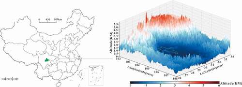
CD is a megacity in China. It is located in the west of the Sichuan Basin and the eastern edge of the Qinghai Tibet Plateau (29°31′N–31°50′ N, 103°00′E–104°42′ E) (Tao et al. 2013). It covers an area of 14,335 km2 and has an average altitude of 500 m. CD is surrounded by mountains with a maximum altitude of > 4 km (Figure 1). At the end of 2018, CD had a population of > 16 million and > 4.8 million vehicles (Sichuan Statistical Yearbook 2019).

Figure 1. Location of the Chengdu in China and three-dimensional terrain in the Chengdu and its surrounding areas.

Data sources and data processing

The meteorological data used in the backward trajectory were GDAS data (ftp://gus.arlhq.noaa.gov/pub/archives/) provided by the National Environmental Prediction Center (NCEP) in 2017, with spatial resolution of 0.5° × 0.5° and time resolution of 6 h. Meteorological data mainly included WS, RH, and temperature and were obtained from Atmospheric Administration (NOAA) and National Centers for Environmental Information (NCEI) (https://www.ncei.noaa.gov), with 2 stations in CD and time resolution of 1 h. The air quality index (AQI) values and standard atmospheric pollutant (i.e., particulate matter with an aerodynamic diameter ≤ 10 µm [PM₁₀], particulate matter with an aerodynamic diameter ≤ 2.5 µm [PM_2.5], O₃, SO₂, NO₂, and CO) concentrations were obtained from the National Urban Air Quality Real-time Publishing Platform (http://106.37.208.233:20035/), with 7 monitoring sites for atmospheric pollutants in CD and time resolution of 1 h.

The AOD is the main indicator of air pollution, and PBLH is an important physical parameter of the atmospheric numerical model and atmospheric environmental assessments (Li et al. 2018). PBLH reflects the movement of air flow and is negatively associated with the AOD. A high PBLH value usually reflects frequent air movement and good air quality (Guo et al. 2016). The AOD data were obtained from the National Aeronautics and Space Administration (NASA) (https://disc.gsfc.nasa.gov), with spatial resolution of 0. 5° × 0. 5° and time resolution of 3 h. The PBLH data were obtained from the European Center for Medium-Range Weather Forecasts (ECMWF) (https://apps.ecmwf.int/datasets),with spatial resolution of 0. 5° × 0. 5° and time resolution of 3 h. Visible Infrared Imaging Radiometer Suite (VIIRS) Nightfire products can detect thermal anomalies in heavy industrial sectors and reflect industrial energy consumption intensity, thus providing a new method for evaluating the effect of urban industrial pollution emissions on air quality (Deetz and Vogel 2017; Franklin et al. 2019; Sun et al. 2020). The National Aeronautics and Space Administration (NASA) Earth Observation Data System (https://earthdata.nasa.gov/earth-observation-data) provides data on VIIRS thermal anomalies at night.

The missing data problem is inevitable in multivariate spatio-temporal big data. For the missing spatio-temporal data, this paper used the Bayesian Gaussian CANDECOMP/PARAFAC (BGCP) tensor decomposition model (Chen, He, and Sun 2019b) to impute missing entries efficiently. Multivariate spatio-temporal big data obtained from different data sources have different spatial and temporal resolutions, and Python was used for processing. For the different spatial resolution data, the first step was region clipping; the array data were then masked using polygons in Python, and the statistical values of the polygons were obtained using the masked array in Python to calculate the average value of CD. The data of time resolution of 3 h were converted into time resolution of 1 h by BGCP. Finally, the hourly, daily, and monthly average values of the corresponding data were calculated.

Random forest algorithm

Random Forest (RF) algorithm is a fusion algorithm based on decision tree classifier proposed by Breiman (Breiman 2001). Random forests (RF) is a new and powerful statistical classifier (Cutler et al. 2007).Advantages of RF compared to other statistical classifiers include (1) very high classification accuracy; (2) flexibility to perform several types of statistical data analysis; (3) processing high-dimensional data without feature selection; (4) easy to implement and parallelize. It has been successfully applied to many fields (Stafoggia et al. 2019; Sun et al. 2016; Wei et al. 2019).

Backward trajectory model

HYSPLIT is a model established by the Air Resources Laboratory in the NOAA (Draxler and Hess 1998). Trajectory cluster analysis is a multivariate statistical analysis technology that is used to divide trajectory data into several categories or clusters. In this study, backward trajectory and trajectory cluster analyses were used. Trajstat, a plug-in of meteoinfo (Wang, Zhang, and Draxler 2009), was used to simulate the backward transport trajectory in CD during the pollution period.

The PSCF method

The PSCF model calculates the potential pollution sources by analyzing the airflow trajectory and pollution threshold. The PSCF value can be interpreted as conditional probability, i.e., the concentration of a given pollutant is greater than the standard level; the unit with a high PSCF value is a region with high potential contribution. The specific calculation is as follows:

(1) $PSC{F}_{ij}=\frac{m_{ij}}{n_{ij}}$(1)

where i and j denote the latitude and longitude, respectively; n_ij represents the total number of air trajectory endpoints passing through the ij cell; and m_ij is defined as the total number of air trajectory endpoints with pollution concentrations exceeding a given criterion value in the same cell (Hsu, Holsen, and Hopke 2003).

To reduce the effect of small n_ij values, the PSCF values were multiplied by an arbitrary weight function W_ij to effectively reflect the uncertainty in the values for these cells (Polissar et al. 1999). WPSCF_ij and W_ij are defined as follows:

(2) $WPSC{F}_{ij}=W_{ij}\times PSC{F}_{ij}$(2)

(3) $W_{ij}=\left\{\begin{array}{c}1.0080<n_{ij}\\ 0.7020<n_{ij}\le 80\\ 0.4210<n_{ij}\le 20\\ 0.05n_{ij}\le 10\end{array}\right\}$(3)

The CWT method

The limitation of the PSCF method is that when the sample concentration is only slightly higher or slightly higher than the standard, the grid cells can have the same PSCF value. As a result, it may be difficult to distinguish between the moderate and intensive sources. In the CWT method (Hsu, Holsen, and Hopke 2003), each grid cell is assigned a weighted concentration by averaging the sample pollutant concentrations that have associated trajectories crossing the grid cell as follows:

(4) $C_{ij}=\frac{1}{{\sum }_{l=1}^M{\tau }_{ijl}}\sum _{l=1}^M{c}_l{\tau }_{ijl}$(4)

where C_ij is the mean weighted concentration in the ij^th cell, l is the index of the trajectory, C_l is the pollutant concentration measured on the arrival of trajectory l, M is the total number of trajectories, and τ_ijl is the time spent in the ij^th cell by trajectory l. In the CWT analysis, the above arbitrary weighting function is also used to reduce the influence of the small n_ij value in the PSCF model.

Previous studies have shown that differences in the trajectory arrival height can have a significant effect on the calculated transport pathway (Jorba et al. 2004; Lyamani, Olmo, and Alados-Arboledas 2005). Furthermore, selection of lower arrival heights may have led to less accurate trajectory calculations due to the incomplete resolution of frictional and turbulent effects near the ground (Sapkota et al. 2005). In this study, 3-day backward trajectories arriving at the Chengdu site with a starting height of 500, 1,000, and 1,500 m were calculated using HYSPLIT model in Trajstat for different pollution periods.PSCF and CWT Require upwind/downwind trajectories, so PSCF and CWT used in combination with HYSPLIT (Hsu, Holsen, and Hopke 2003).

Results

Air quality variation characteristics

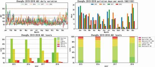
The AQI data for CD were analyzed according to the national environmental quality standard(MEP, 2012a). Figure 2 shows the changes in the daily average concentration, monthly pollution peak episodes, and annual air quality level proportion in CD during 2015‒2018. From the daily change in AQI, it can be seen that the change was generally U-shaped and that the AQI values during January‒February and November‒December were larger. From the change in monthly pollution days, it can be seen that pollution mainly occurred in January, February, March, May, July, August, November, and December (in last 2 years, the polluted days are > 10 d). From the change in the annual air quality level proportion, it can be seen that, since 2016, the air quality has improved, the proportion of fine weather has gradually increased, and the proportion of pollution has gradually decreased.

Figure 2. Variation Characteristics of daily average AQI concentration, distribution of pollution days and proportion of AQI grade in Chengdu from 2015 to 2018.

Random forest classification

Air pollution data of CD in 2017 were evaluated using RF classification, and the results are shown in Table 1.

Table 1. Random forest classification of air pollutants in Chengdu 2017.

Cluster		PM2.5(μg·m^−3)	PM10(μg·m^−3)	SO2(μg·m^−3)	NO2(μg·m^−3)	CO(μg·m^−3)	O3(μg·m^−3)
1	average	129.24 ± 29.08	185.34 ± 39.05	16.11 ± 4.29	75.39 ± 13.00	1.56 ± 0.25	50.37 ± 31.15
	days	38	38	38	38	38	38
2	average	65.41 ± 20.65	102.45 ± 28.85	13.00 ± 3.65	60.48 ± 9.52	1.07 ± 0.17	57.67 ± 37.41
	days	92	92	92	92	92	92
3	average	26.72 ± 12.69	45.96 ± 18.45	8.96 ± 1.55	40.02 ± 8.75	0.78 ± 0.15	79.49 ± 34.05
	days	135	135	135	135	135	135
4	average	36.08 ± 16.17	63.38 ± 25.26	10.09 ± 2.87	48.58 ± 12.59	0.83 ± 0.13	172.66 ± 31.79
	days	89	89	89	89	89	89
5	average	214.45 ± 41.86	320.55 ± 67.29	18.55 ± 4.66	93.55 ± 19.23	2.19 ± 0.30	39.27 ± 24.92
	days	11	11	11	11	11	11

According to the national environmental quality standard (MEP, 2012b) (Table 2), the air pollution in CD was mainly due to PM_2.5, PM₁₀, NO₂, and O₃. The results of classification were divided into five categories: cluster 5, serious pollution; cluster 1, moderate pollution; cluster 4, moderate pollution (mainly ozone pollution); cluster 2, slight pollution; and cluster 3, excellent air quality.

Table 2. Basic concentration limit of ambient air pollutants.

		Concentration Limit (μg·m-3)
Pollutant	Mean time	level I	level II
SO2	24 hour	50	150
NO2	24 hour	80	80
CO	24 hour	4	4
O3	8 hour	100	160
PM10	24 hour	50	150
PM2.5	24 hour	35	75

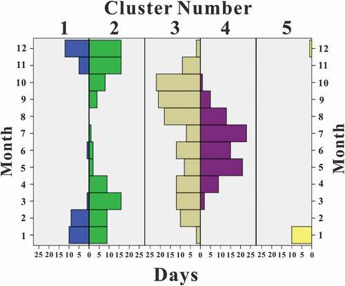
The monthly cluster classification frequency chart and specific distribution data are shown in Figure 3. Cluster 5 showed that serious pollution occurred mainly in January and December 2017, mainly because PM_2.5, PM₁₀, and NO₂ far exceeded the secondary standard (Table 2). Cluster 1 showed that moderate pollution occurred mainly in January, February, December, and November and to a small degree in March and June, which was mainly reflected in PM_2.5 and PM₁₀ concentrations that exceeded the secondary standard. Cluster 4 showed ozone pollution, which exceeded the secondary standard, mainly in (May‒August). Cluster 3 indicated the air quality was excellent, mainly during August‒October. Cluster 2 showed that slight pollution mainly occurred in March, November, and December, which showed that PM_2.5 and PM₁₀, approached the secondary standard. According to the similarity principle, the 2017 pollution analysis was divided into four periods; the serious pollution period was January, February and December, the ozone pollution period was May‒August, and the light pollution period was March and November. April, September, and October were periods with good air quality.

Figure 3. Classification frequency chart of air pollutants in Chengdu 2017.

Spatio-temporal trajectories analysis of pollutant

We calculated 72 h air mass back trajectories arriving at the CD (Figure 4).The method used in trajectory clustering was based on the GIS-based software TrajStat.The duration of the back trajectories of each pollution periods in 2017 were from November 29 to February 28, from April 29 to August 31, from February 27 to March 31, and from October 30 to November 30 respectively. To further study the spatio-temporal trajectories of various types of air pollutant in the each pollution period, the PM_2.5, NO₂, and PM₁₀ thresholds were set at 75 μg·m⁻³, 80 μg·m⁻³, and 150 μg·m⁻³, respectively. During the ozone pollution period, the threshold value of O₃ was 160 μg·m⁻³. In the light pollution period, the PM_2.5 and PM₁₀ thresholds were set to 75 μg·m⁻³ and 150 μg·m⁻³, respectively. The trajectories of each period were statistically analyzed, and the average concentration of the main pollutants, main passing areas, probability of occurrence, and characteristics of pollution trajectories corresponding to various trajectories were calculated based on the GIS-based software TrajStat (Figure 5, Figure 6, and Figure 7).

Figure 4. The air spatio-temporal trajectories of each pollution period in Chengdu 2017.

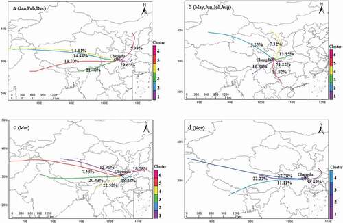
Figure 5. The pollutants (PM_2.5, PM₁₀ and NO₂) of occurrence probability and corresponding concentration of each air trajectory during serious pollution period in Chengdu 2017.

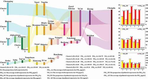
Figure 6. The O₃ of occurrence probability and corresponding concentration of each air trajectory during O₃ pollution period in Chengdu 2017.

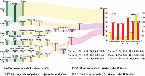
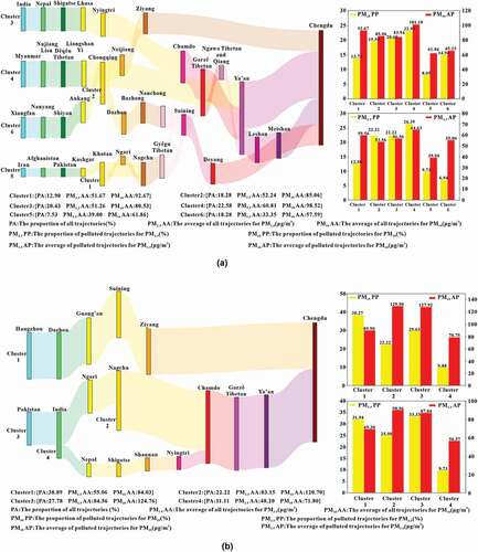
Figure 7. The pollutants (PM_2.5, PM₁₀) of occurrence probability and corresponding concentration of each air trajectory during slight pollution period in Chengdu 2017.

Serious pollution period

Six trajectory types affected air quality in CD during the study period. As can be seen from Figures 4a and 5, clusters 2, 4, and 5 were from India, etc., and were introduced into CD via Tibet, Sichuan Garzê Tibetan, and Ya’an, accounting for 14.44%, 14.81%, and 13.70%, respectively; cluster 3 came from Bhutan, India, and Myanmar, which was introduced into CD via Yunnan Dêqên Tibetan, Sichuan Garzê Tibetan, and Ya’an, accounting for 21.48%; cluster 1 came from Chongqing, accounting for the highest proportion (29.63%), and cluster 6 came from Inner Mongolia and Shaanxi, accounting for 5.93%. In the statistical analysis of pollution trajectories, the air quality of cluster 3 had the highest PM_2.5, PM₁₀, and NO₂ concentrations, with averages of 167.91 μg·m⁻³, 272.55 μg·m⁻³, and 298.26 μg·m^−3, respectively; cluster 1 and cluster 3 air quality pollution trajectories accounted for > 20%; the proportion of pollution trajectories in cluster 6 was negligible, and the proportion of air quality pollution in clusters 2, 4, and 5 was 10%–20%.

Ozone pollution period

Ozone pollution mainly occurred during May‒August. As can be seen from Figures 4b and 6, the trajectory of cluster 6 accounted for the largest proportion, reaching 51.22%, and the pollution trajectory also accounted for the largest proportion, reaching 52.27%, which mainly came from Guang’an, Chongqing, and Ziyang. The pollution trajectories of cluster 4 had the highest average O₃ concentration of 249.25 μg·m⁻³, most of which came from Inner Mongolia and entered CD through Ningxia Province, Gansu Province, Guangyuan, Mianyang, and Deyang, accounting for only 6.06%. The pollution trajectories of cluster 1 came from Myanmar and entered CD through Yunnan Province, Sichuan Liangshan, Sichuan Garzê Tibetan, Ya’an, Leshan, and Meishan, accounting for 15.91%; The pollution trajectories of cluster 2 came from Xinjiang Aksu, passed through Qinghai Province and Sichuan Ngawa Tibetan, and Qiang, and entered CD, accounting for 3.79%. The pollution trajectories of cluster 3 came from Hubei Shiyan, and entered CD through Chongqing, Dazhou, Nanchong, Suining, and Deyang, accounting for 6.06%. The pollution trajectories of cluster 5 came from Guangxi Baise, via Guizhou Province, Yunnan Zhaotong, Yibin, Leshan, Zigong, and Meishan, and entered CD, accounting for 15.91%.

Slight pollution period

Slight pollution mainly occurred in March and November, and the main pollution components were PM_2.5 and PM₁₀. According to Figures 4c and 7a, the pollution trajectories were mainly concentrated in clusters 2, 3, and 4 in March. The pollution trajectories of cluster 4 had the highest average PM_2.5 and PM₁₀ concentrations, reaching 64.63 μg·m⁻³ and 101.10 μg·m⁻³, respectively (accounting for 26.39% and 22.99% respectively), which mainly came from Myanmar, through Yunnan Province, Sichuan Liangshan, Ya’an, Leshan, and Meishan, and entered CD. Cluster 2 came from Chongqing and entered CD through Neijiang and Ziyang, and the pollution trajectories of PM_2.5 and PM₁₀ accounted for 22.22% and 19.54%, respectively. Cluster 3 came from India and entered CD through Nepal, Tibet, Sichuan Garzê Tibetan, and Ya’an, and the pollution trajectories of PM_2.5 and PM₁₀ accounted for 22.22% and 20.69% respectively.

According to Figures 4d and 7b, the pollution trajectories in November were mainly concentrated in clusters 1, 2, and 3, and the proportions of the pollution trajectories were > 20%. Cluster 1 came from Shangxi Hanzhong, entered CD via Dazhou, Guang’an, Suining, and Ziyang, and had the highest pollution trajectory proportions of PM_2.5 and PM₁₀, accounting for 31.94% and 38.27%, respectively. The pollution trajectories of cluster 2 had the highest average PM_2.5 and PM₁₀ concentrations, reaching 90.06 μg·m⁻³ and 129.50 μg·m⁻³, respectively (accounting for 25.00% and 22.22%, respectively) which mainly came from Tibet Nagchu, through Sichuan Chamdo and Sichuan Garzê Tibetan, and entered CD. The pollution trajectories of cluster 3 had the highest average PM_2.5, and PM₁₀ concentrations, reaching 87.04 μg·m⁻³ and 127.92 μg·m⁻³, respectively, and mainly came from Pakistan, India, Tibet, and Ya’an, and entered CD.

Spatio-temporal distribution of pollution sources

Serious pollution period

The PM_2.5, PM₁₀, and NO₂ threshold values were set to 75 μg·m⁻³, 150 μg·m⁻³, and 80 μg·m⁻³, respectively, to calculate the pollution trajectories. The results of the potential sources of pollution trajectories and the distribution of pollution concentration contributions are shown in Figure 8.

Figure 8. Spatial distribution of WPSCF and WCWT values of PM_2.5, PM₁₀ and NO₂ of serious pollution period in Chengdu 2017.

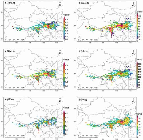
When the WPSCF of PM_2.5 was > 0.6, it indicated that the region contributed significantly to PM_2.5 pollution and that is was the main potential source area. It can be seen from Figure 8a that it was mainly concentrated in CD and its surrounding areas, such as Sichuan Garzê Tibetan, Ya’an, Meishan, Leshan, Yibin, and Ziyang, with sporadic high values in India, Nepal, Myanmar, and Tibet. The WCWT can more clearly reflect the concentration contributions of different potential source areas, whereby the greater the WCWT value, the greater the contribution of the area to the PM_2.5 concentration. As can be seen from Figure 8b, it was mainly concentrated in two areas: the area of CD and its surrounding areas (including Sichuan Garzê Tibetan, Ya’an, Meishan, Leshan, Yibin, Ziyang, Neijiang, Zigong, Luzhou, and Chongqing); and India, Myanmar, and southern Tibet. In conclusion, the air trajectories from India, Myanmar, and Chongqing may have had a certain impact on PM_2.5 pollution during this period.

When the WPSCF of PM₁₀ was > 0.4, it indicated that the contribution of pollution in this area was larger and that it was the most important potential source area. From the Figure 8c, the distribution was similar to PM_2.5, and was mainly concentrated in Sichuan Garzê Tibetan, CD, Ya’an, Meishan, Leshan, Yibin, and Luzhou. Sporadic high values appeared in Chongqing, southern Tibet, Myanmar, India, and Nepal. The potential sources of high pollution concentrations of WCWT were mainly reflected in two areas: (1) India, Myanmar, southern Tibet, Yunnan Dêqên Tibetan, and (2) CD and its surroundings, including Sichuan Garzê Tibetan, Ya’an, Meishan, and Neijiang. From the analysis of trajectory and concentration distribution, the air trajectories from India and Myanmar may have had a certain impact on PM₁₀ pollution during this period (Figure 8d).

The WPSCF of NO₂ was > 0.4, which was the main potential source area. As shown in Figure 8e, high values were found in CD, Meishan, Yibin, Leshan, and Zigong, with sporadic high values in Hanzhoung, Ankang, Chongqing, Xiangxi, Tongren, Burma, southern Tibet, and Nepal. The areas with high pollution concentration reflected by WCWT were mainly concentrated in two regions: (1) India, Myanmar, and southern Tibet; and (2) CD and its surrounding areas, including Sichuan Garzê Tibetan, Ya’an, Meishan, Leshan, Zigong, Neijiang, Ziyang, Yibin, Luzhou, Suining, and Guang’an (Figure 8f). From the analysis of trajectories and concentration distribution, the air trajectories from India and Myanmar, Chongqing, and Inner Mongolia may have had a certain impact on NO₂ pollution during this period.

Ozone pollution period

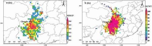
The O₃ threshold value was set to 160 μg·m⁻³ to calculate pollution trajectories. The results of the potential sources of pollution trajectories and the distribution of pollution concentration contributions are shown in Figure 9. When the WPSCF value was > 0.4, it indicated that the contribution of the area to ozone pollution in CD was relatively large, and that it was the main potential source area. The WPSCF O₃ high-value area was mainly distributed in the urban agglomeration of the Sichuan Basin, followed by the sporadic high-value area at the junction of Sichuan and Yunnan and the Kunming-Honghe belt in Yunnan. The WCWT can more intuitively determine the concentration contribution of different potential source areas. Figure 9b shows that some areas of the Sichuan Basin urban agglomeration, Chongqing, Sichuan Liangshan, Yunnan, and Guizhou contributed the most to the O₃ in Chengdu.

Figure 9. Spatial distribution of WPSCF and WCWT values of O₃ of Ozone pollution period in Chengdu 2017.

Slight pollution period

March and November were the slight pollution periods, and the PM_2.5 and PM₁₀ threshold values were set to 75 μg·m⁻³ and 150 μg·m^−3, respectively, to calculate the pollution trajectories; the results are shown in Figure 10.

Figure 10. Spatial distribution of WPSCF and WCWT values of PM_2.5 and PM₁₀ of light pollution period in Chengdu 2017.

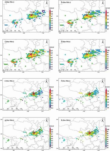
In March, the potential sources of PM_2.5 pollution were in CD and its surrounding areas, and sporadically high values were also found in Myanmar and India (Figure 10a). The high concentration areas reflected by WCWT were mainly concentrated in CD and its surrounding areas, and sporadic high values were observed in Myanmar, India, and Chongqing (Figure 10b). It can be seen that the air trajectories from Myanmar and Chongqing may have contributed to PM_2.5. The potential source area of PM₁₀ pollution was consistent with that of PM_2.5 (Figure 10c), whereas the high concentration area of WCWT was mainly reflected in CD and its surrounding areas. There were some high values in Myanmar and India (Figure 10d). Therefore, the air trajectories from Myanmar may have contributed to PM₁₀ during this period.

In November, the potential sources of PM_2.5 and the high concentration areas of WCWT were mainly in CD and the surrounding areas (Figure 10e and Figure 10f). The pollution potential sources and pollution concentration contribution of PM₁₀ were consistent with that of PM_2.5 (Figures 10g and Figure 10h). This shows that the pollution in this period was slightly affected by the external air trajectories.

Air pollutants cause analysis in internal Chengdu

Analysis of spatio-temporal characteristics of pollutants

Figure 11 shows the hourly, daily, and monthly variations in the main pollutants in CD in 2017. Figure 12 shows the hourly variations in meteorological data (temperature, RH, and WS), AOD, PBLH, and pollutant gases. In CD, thermal anomaly data usually refer to abnormal points for which the temperature is usually > 500 K (Schroeder et al. 2014), reflecting industrial combustion at nights in CD. Figure 13 shows the distribution of thermal anomaly points in several typical industrial fields. The following results were obtained from Figures 4 and 5: (1) The daily changes in PM_2.5, PM₁₀ and NO₂ concentrations exhibited the “double valley and double peak” type, with peak values at approximately 10:00 and 23:00. PM_2.5 and PM₁₀ valley values occurred at 07:00 and 19:00, respectively; NO₂ valley values occurred at approximately 07:00 and 17:00, and were higher at night than in the daytime and lower than in the early morning than in the evening. The main reasons are that the peak of the human activity begins at 07:00, the exhaust emissions of automobiles increase, and the ground temperature increases gradually after sunrise. Furthermore, the WS was lower; artificial emission sources increased, thereby increasing the pollutant concentration and reaching the first peak at approximately 10:00. (2) In the afternoon, the daily temperature reached the maximum; the surface temperature, air flow, WS, and PBLH value increased; and RH and the AOD value decreased. The meteorological conditions in this stage were conducive to pollution diffusion, resulting in a gradual decrease in pollutant concentrations. NO₂ decreased to a minimum at 17:00, PM_2.5 and PM₁₀ decreased to a minimum at 19:00, and the second valley appeared. (3) The peak time of end of typical work day shift began at 17:00. The ground temperature began to drop, resulting in an inversion layer. The RH began to increase, WS began to decline, AOD value continued to increase, and PBLH value continued to decline. The meteorological conditions at this stage were not conducive to pollution diffusion. The emissions of factories at night (Figure 13) can easily cause the accumulation of pollutants, and the second peak of PM_2.5, PM₁₀, and NO₂ appeared at 23:00. (4) After midnight, human activities decreased considerably and the pollution concentration gradually decreased to reach the trough at 07:00. Because of factory discharge after midnight (Figure 13), the RH was relatively high, the WS and temperature were lower, the AOD value was larger, the PBLH value was smaller; it was not easy for pollution to spread and therefore the pollution concentration decreased slightly. (5) The daily variation in the O₃ concentration showed a “single peak.” The temperature gradually increased from 10:00; the O₃ concentration gradually increased, reached a peak at 16:00, and then gradually decreased. The O₃ concentration was positively correlated with temperature.

Figure 11. The hourly, daily and monthly variations of PM_2.5, PM₁₀, NO₂ and O₃ in Chengdu in 2017.

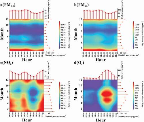
Figure 12. The hourly variation of meteorological data (temperature, relative humidity, and wind speed), AOD, PBLH and pollutant gases (PM_2.5, PM₁₀, NO₂ and O₃) in Chengdu 2017.

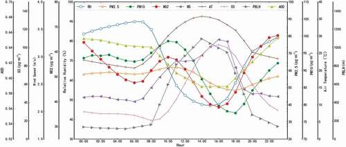
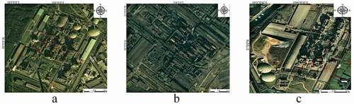
Figure 13. Distribution of thermal anomalies in typical industrial areas: a is a cement plant; b is a steel plant; c is a manufacturing plant.

Relationship between wind speed and pollution

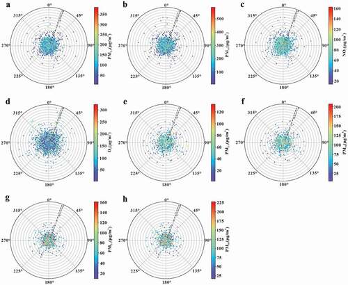
During the severe pollution period, the hourly pollution distribution was relatively intensive; the high concentrations of PM_2.5, PM₁₀, and NO₂ were mainly concentrated in the low WS area (0–3 m·s⁻¹) (Figures 14a‒c). This indicates that the low WS in this period was not easily associated with pollution diffusion, resulting in pollution accumulation. During the ozone pollution period, the high O₃ concentration was mainly in the WS range of 0–3 m·s⁻¹ (Figure 14d). In the light pollution period of March and November, the hourly pollution distribution was relatively scattered, indicating that the hourly WS was high during this period. In March, the high PM_2.5 and PM₁₀ concentrations were mainly concentrated in the area with WS of 0–2 m·s⁻¹ (Figures 14c and Figure 14f). In November, high PM_2.5 and PM₁₀ concentrations were mainly concentrated in the low WS area (0–3 m·s⁻¹) (Figure 14g and Figure 14h), indicating that the low WS decelerated the easy spread of pollution. Because of the low hourly WS in CD (Figure 12), the pollutant air mass may reach CD along the air flow direction and particulate matter will accumulate and not easily diffuse, resulting in an increase in pollutant concentrations in the urban area and the negatively affecting the surrounding air quality.

Figure 14. Hourly distribution relationship between wind speed and pollution in each pollution period.

From the above analysis, in addition to the air pollution emitted internally, there may be external air pollution input in Chengdu. From the diagram of pollution source analysis, the main pollution was still caused by internal emissions, and there were some external inputs, which were mainly reflected in PM2.5,PM10 and NO2 in December, January and February. The emission of internal air pollution may mainly occur due to the following reasons: 1) the population of CD is 16 million and 4.8 million vehicles, so the emission of working and living pollution contributes greatly to the air pollution; 2) Meteorological Problems: the atmospheric pollution is mainly concentrated in the low wind speed, which shows that the meteorology in CD is in a stagnant state, which is not conducive to the diffusion of atmospheric pollution; 3) As for the terrain, Chengdu is surrounded by mountains, which is prone to deposition of air pollution; 4) Heavy pollution at night may be due to industrial emissions at night; At night, the concentration of AOD is large, which is easy to cause aerosol secondary pollution, which is also the reason for aggravating night pollution.

Discussions

The possibility of external pollution input is obtained by trajectory analysis. From the method given in this paper, there may be some uncertainty.Two important choices in back trajectory modeling are the selection of arrival height and time length of trajectories(Borge et al. 2007). Back trajectories calculated with HYSPLIT at different starting heights have different paths with increasing travel times(Hsu, Holsen, and Hopke 2003).Trajectories cluster analysis in general is not a purely objective classification method, since the selection of the clustering algorithm, variables, metric and number of clusters are subjective choices (Brankov, Rao, and Porter 1998; Dorling, Davies, and Pierce 1992; Moy, Dickerson, and Ryan 1994; Stohl 1998).In certain cases, back trajectory modeling has been used, in combination with chemical speciation and/or synoptic weather maps to identify long-range transport sources of polluted air masses that may have an impact on local air pollution (Rodrıguez et al. 2001; Salvador et al. 2004; Viana et al. 2002). Interestingly, this findings in our study are consistent with some studies. Such as: 1) In DJF(December, January and February) desert dust derived predominately from northwestern India and Pakistan, can be transported to the western Tibetan Plateau (TP), and dust particles mix with local polluted aerosols(Liu et al. 2008). 2) The dust aerosols were mostly observed in the altitude range of 4–6 km over the TP, with the highest value over the Qaidam Basin in the northeast, and the high value area could extend to the east slope of the TP, west of Sichuan Province(Liao et al. 2021). 3) During the biomass burning period, the prevailing westerly airflow and the relatively large amount of smoke emitted in northeastern India and Burma led to the potential for long-range transport of smoke from these regions to the the Yunnan-Guizhou Plateau (Zhu et al. 2017). Many studies have shown that India has a certain impact on pollution and precipitation in Tibet and Yunnan (Chen et al. 2014, 2019a, 2008; Cong et al. 2010; Ji et al. 2015; Kang, Cong, and Wang et al. 2019; Yin et al. 2019). It is proved that these methods are suitable for long-distance atmospheric trajectory transmission in Chengdu, and proved the validity of the results of this study.

The possible external pollution trajectories and sources during various pollution periods in CD were discussed. During the ozone pollution period, O₃ pollution was mainly concentrated in CD and its surrounding areas, with less long-distance transmission. During the main pollution period, PM_2.5, PM₁₀, and NO₂ came not only from CD and the surrounding areas but also may be from air pollution from India to CD and India through Tibet and from Myanmar to CD through Dêqên Tibetan of Yunnan. During the slight pollution period, PM_2.5 and PM₁₀ were mainly concentrated in CD and the surrounding areas, with less impact from external pollution.

Based on the multivariate spatio-temporal big data, this study analyzed the hourly, daily, and monthly variations in pollutant gases in CD and obtained the law and basic characteristics of daily variations in pollutant gases in CD. This result indicates that the air pollutant concentration could have been influenced largely by human activities regularity, traffic emissions, and factories discharge at night in internal CD. We can see from the monthly variation in Figure 11 that the higher concentrations of PM_2.5, PM₁₀, and NO₂ mainly occurred during December, January, and February; the concentrations of PM_2.5 and PM₁₀ were also high in March and November, and the high O₃ concentrations mainly occurred during May‒August, which were consistent with the RF classification. The distribution relationship between the hourly average pollutant gases and the hourly average WS in each pollution period is discussed. The results show that the pollutant gases in the range of low WS, proving that the low WS in CD is not conducive to the diffusion of pollutant gases and that it easily causes urban pollution accumulation, which is consistent with the finding of a previous study (Liao et al. 2018).

Conclusion

In this study, the Spatial-temporal trajectory of air pollution, the Spatial-temporal characteristics of air pollution, and the causes of air pollution were analyzed in details during various pollution periods in CD. The main conclusions are as follows:

(1) During 2015‒2018, the diurnal variation in AQI was U-shaped in CD. Since 2016, the air quality has improved, the proportion of fine weather has gradually increased, and the proportion of pollution has gradually decreased.

(2) Air pollution in CD can be divided into three periods. The main pollution periods were January, February, and December, and the main pollution components were PM_2.5, PM₁₀, and NO₂; the ozone pollution period was during May‒August; the slight pollution periods were March and November, and the main pollution components were PM_2.5 and PM_10.

(3) During the serious pollution period, the PM_2.5, PM₁₀, and NO₂ sources were mainly concentrated in the CD and surrounding areas. PM_2.5 from India, Myanmar, and Chongqing may have contributed to PM_2.5 pollution in CD; PM₁₀ from India and Myanmar may have contributed to the PM₁₀ pollution in CD; NO₂ from India, Myanmar, Chongqing, and Inner Mongolia may have contributed to NO₂ pollution in CD. During the ozone pollution period, urban agglomeration in Sichuan Basin, Chongqing, Sichuan Liangshan, and some areas in Yunnan and Guizhou Provinces contributed significantly to ozone pollution in CD. In the slight pollution period, in March, the PM_2.5 source was mainly concentrated in the CD and its surrounding areas. Pollution from Myanmar and Chongqing may have made a small contribution to PM_2.5 pollution in CD; the PM₁₀ source was mainly concentrated in CD and surrounding areas. Pollution from Myanmar may have made a small contribution to the PM₁₀ pollution in CD. In November, the PM_2.5, and PM₁₀ sources were mainly concentrated in CD and its surrounding areas, with little external influence.

(4) Regarding the hourly variations in main pollutants in CD, the PM_2.5, PM₁₀ and NO₂ concentrations presented a “double valley and double peak” pattern, with the peak values at approximately 10:00 and 23:00, valley values of PM_2.5 and PM₁₀ at approximately 07:00 and 19:00, and valley values of NO₂ at approximately 07:00 and 17:00. The hourly variation in the O₃ concentration presented a “single peak,” with the temperature gradually increasing and the O₃ concentration gradually increasing from 10:00. The O₃ concentration peaked at 16:00 and then gradually decreased. This was related to work and lifestyle, night industrial emissions, and meteorological conditions in CD.

(5) During the severe pollution period, high PM_2.5, PM₁₀, and NO₂ concentrations were concentrated in the low WS area (0‒3 m·s⁻¹). During the ozone pollution period, high O₃ was concentrated in the WS range (0‒3 m·s⁻¹). During the slight pollution period, high PM_2.5 and PM₁₀ concentrations were mainly concentrated in the low WS zone (0‒2 m·s⁻¹) in March, and high PM_2.5, and PM₁₀ concentrations were mainly concentrated in the low WS zone (0‒3 m·s⁻¹) in November. This shows that the lower WS in CD makes the pollution difficult to spread and easily accumulated.

Taking CD as an example, this study analyzed the influence of internal pollution characteristics and external pollution source areas on megacities in basin areas surrounded by mountains, which provides a scientific basis for air pollution control and regional joint prevention and control in different pollution periods in CD. It also provides a basis for future research on the pollution characteristics and sources in megacities in basin areas surrounded by mountains.

Disclosure statement

No potential conflict of interest was reported by the author(s).

Data availability statement

The data that support the findings of this study are available from the corresponding author upon reasonable request. http://sweb.cdutetc.cn/tmgc/wxj/20220407.rar

Supplementary material

Supplemental data for this paper can be accessed on the publisher’s website.

Additional information

Funding

This research was funded by the National Key R&D Program of China (2017YFC0601505) by Ke Guo, Chinese National Natural Science Foundation (41672325, 41602334) by Ke Guo, and the Geomathematics Key Laboratory of Sichuan Province Foundation (scsxdz2021zd01, scsxdz2021yb03) by Ling Chen and XingJie Wang.

Notes on contributors

Xingjie Wang

Xingjie Wang received a B.S. degree in Automation from Kunming University of Science and Technology, Kunming, China, in 2003, and an M.S. degree in Computer application technology from Kunming University of Science and Technology, Kunming, China, in 2006. He is currently working toward a Ph.D. degree with Geodetection and Information Technology, Chengdu University of Technology, Chengdu, China.

He is currently a Professor with College of Engineering and Technology, Chengdu University of Technology. His research interests include remote sensing image processing, earth exploration, and spatio-temporal big data.

Ling Chen

Ling Chen received a B.S. degree in mathematics education from Southwest Normal University, Chongqing, China, in 1992, and an M.S. degree in applied mathematics, in 2003, and a Ph.D. degree in geodetection and information technology, in 2011, both from the Chengdu University of Technology, Chengdu, China.

She is currently a Professor with the Geomathe-matics Key Laboratory of Sichuan Province, Chengdu University of Technology. Her research interests include remote sensing image processing, earth exploration, and information technology.

Ke Guo

Ke Guo received a B.S. degree in mathematics from Chengdu Geological College, Chengdu, China, in 1985, an M.S. degree in geomathematics from Chengdu Geological College, Chengdu, China, in 1990, and a Ph.D. degree in mineral resource prospecting and exploration from the Chengdu University of Technology, Chengdu, China, in 2005.

He is a Professor and Doctoral Supervisor with the Chengdu University of Technology, Chengdu, China. He is an Academic and Technical Leader of Sichuan province and enjoy special subsidies from the State Council Government. He is currently the Head of the teaching team of mathematics geology in Sichuan province, and the Head of the scientific research and innovation team of high-level resources and environment in Sichuan province. He has long been involved in the teaching and scientific research of quantitative evaluation and prediction of resources and environment.

Bingli Liu

Bingli Liu received a B.S. degree in Mathematics and Applied Mathematics, in 2003, and an M.S. degree in computational mathematics, in 2006, and a Ph.D. degree with Geodetection and Information Technology, in 2012, all from Chengdu University of Technology, Chengdu, China.

He is currently a associate professor with the Geomathe-matics Key Laboratory of Sichuan Province, Chengdu University of Technology. Her research interests include mathematical geology, earth exploration, and spatio-temporal big data.

References

- Borge, R., J. Lumbreras, S. Vardoulakis, P. Kassomenos, and E. Rodriguez. 2007. Analysis of long-range transport influences on urban PM10 using two-stage atmospheric trajectory clusters. Atmos. Environ. 41 (21):4434–50. doi:https://doi.org/10.1016/j.atmosenv.2007.01.053.
- Brankov, E., S. T. Rao, and P. S. Porter. 1998. A trajectory-clustering correlation methodology for examining the long-range transport of air pollutants. Atmos. Environ. 32 (9):1525–34. doi:https://doi.org/10.1016/S1352-2310(97)00388-9.
- Breiman, L. 2001. Random forests. Mach. Learn. 45 (1):5–32. doi:https://doi.org/10.1023/A:1010933404324.
- Burnett, R., H. Chen, M. Szyszkowicz, N. Fann, B. Hubbell, C. A. Pope, J. S. Apte, M. Brauer, A. Cohen, S. Weichenthal, et al. 2018. Global estimates of mortality associated with long-term exposure to outdoor fine particulate matter. Proc Natl Acad Sci 115 (38):9592–97. doi:https://doi.org/10.1073/pnas.1803222115.
- Calderon-garciduenas, L., R. J. Kulesza, R. L. Doty, A. D’Angiulli, R. Torres-Jardón. 2015. Megacities air pollution problems: Mexico City Metropolitan Area critical issues on the central nervous system pediatric impact. Environ. Res. 137:157–69. doi:https://doi.org/10.1016/j.envres.2014.12.012.
- Chen, F. H., X. M. Chen, J. H. Chen, A. Zhou, D. Wu, L. Tang, X. Zhang, X. Huang, J. Yu. 2014. Holocene vegetation history, precipitation changes and Indian Summer Monsoon evolution documented from sediments of Xingyun Lake, south-west China. J. Quat. Sci. 29 (7):661–74. doi:https://doi.org/10.1002/jqs.2735.
- Chen, X. Y., Z. C. He, and L. J. Sun. 2019b. A Bayesian tensor decomposition approach for spatiotemporal traffic data imputation. Transp. Res. Part C: Emerg.Technol. 98:73–84. doi:https://doi.org/10.1016/j.trc.2018.11.003.
- Chen, P. F., S. C. Kang, J. H. Yang, C. Li, J. Guo, L. Tripathee, S. Kang. 2019a. Spatial and temporal variations of gaseous and particulate pollutants in Six Sites in Tibet, China, during 2016-2017. Aerosol Air Qual. Res. 19 (3):516–27. doi:https://doi.org/10.4209/aaqr.2018.10.0360.
- Chen, F. H., Z. C. Yu, M. L. Yang, E. Ito, S. Wang, D. B. Madsen, X. Huang, Y. Zhao, T. Sato, H. John B. Birks, et al. 2008. Holocene moisture evolution in arid Central Asia and its out-of-phase relationship with Asian monsoon history. Quat Sci Rev 27 (3–4):351–64. doi:https://doi.org/10.1016/j.quascirev.2007.10.017.
- Cheng, M. D., P. K. Hopke, and Y. Zeng. 1993. A receptor methodology for determining source regions of particle sulfate composition observed at Dorset, Ontario. J. Geophys. Res. Atmos. 98 (D9):16839–49. doi:https://doi.org/10.1029/92JD02622.
- Cong, Z. Y., S. C. Kang, S. P. Dong, X. D. Liu, and D. H. Qin. 2010. Elemental and individual particle analysis of atmospheric aerosols from high Himalayas. Environ. Monit. Assess. 160 (1–4):323–35. doi:https://doi.org/10.1007/s10661-008-0698-3.
- Cutler, D. R., T. C. Edwards, K. H. Beard, A. Cutler, K. T. Hess, J. Gibson, J. J. Lawler. 2007. Random forests for classification in ecology. Ecol. 88 (11):2783–92. doi:https://doi.org/10.1890/07-0539.1.
- Deetz, K., and B. Vogel. 2017. Development of a new gas-flaring emission dataset for southern West Africa. Geosci. Model Dev. 10 (4):1607–20. doi:https://doi.org/10.5194/gmd-10-1607-2017.
- Dorling, S. R., T. D. Davies, and C. E. Pierce. 1992. Cluster analysis:a technique for estimating the synoptic meteorological controls on air and precipitation chemistry-method and applications. Atmos. Environ. 26 (14):2575–81. doi:https://doi.org/10.1016/0960-1686(92)90110-7.
- Draxler, R. R., and G. D. Hess. 1998. An overview of the hysplit-4 modeling system for trajectories. Aust. Meteorol. Mag. 47:295–308.
- Franklin, M., K. Chau, L. J. Cushing, and J. E. Johnston. 2019. Characterizing flaring from unconventional oil and gas operations in South Texas using satellite observations. Environ. Sci. Technol. 53 (4):2220–28. doi:https://doi.org/10.1021/acs.est.8b05355.
- Guo, J. P., M. J. Deng, S. Lee, F. Wang, Z. Li, P. Zhai, H. Liu, W. Lv, W. Yao, X. Li, et al. 2016. Delaying precipitation and lightning by air pollution over Pearl River Delta. PartI:observational analyses. J. Geophys. Res. Atmos. 121 (11):6472–88. doi:https://doi.org/10.1002/2015JD023257.
- Hou, X. W., B. Zhu, K. R. Kumar, and W. Lu. 2019. Inter-annual variability in fine particulate matter pollution over China during 2013-2018: Role of meteorology. Atmos. Environ. 214:116842. doi:https://doi.org/10.1016/j.atmosenv.2019.116842.
- Hsu, Y. K., T. M. Holsen, and P. K. Hopke. 2003. Comparison of hybrid receptor models to locate PCB sources in Chicago. Atmos. Environ. 37 (4):545–62. doi:https://doi.org/10.1016/S1352-2310(02)00886-5.
- Huang, X. J., J. K. Zhang, B. Luo, L. Wang, G. Tang, Z. Liu, H. Song, W. Zhang, L. Yuan, Y. Wang, et al. 2018. Water-soluble ions in PM 2.5 during spring haze and dust periods in Chengdu, China: Variations, nitrate formation and potential source areas. Environ. Pollut. 243:1740–49. doi:https://doi.org/10.1016/j.envpol.2018.09.126.
- Ji, Z. M., S. C. Kang, Z. Y. Cong, Q. Zhang, T. Yao. 2015. Simulation of carbonaceous aerosols over the Third Pole and adjacent regions: Distribution, transportation, deposition, and climatic effects. Clim. Dyn. 45 (9–10):2831–46. doi:https://doi.org/10.1007/s00382-015-2509-1.
- Jorba, O., C. Perez, F. Rocadenbosch, and J. M. Baldasano. 2004. Cluster analysis of 4-day back trajectories arriving in the Barcelona area, Spain, from 1997 to 2002. J. Appl. Meteorol. 43 (6):887–901. doi:https://doi.org/10.1175/1520-0450(2004)043<0887:CAODBT>2.0.CO;2.
- Kanakidou, M., N. Mihalopoulos, T. Kindap, U. Im, M. Vrekoussis, E. Gerasopoulos, E. Dermitzaki, A. Unal, M. Koçak, K. Markakis, et al. 2011. Megacities as hot spots of air pollution in the East Mediterranean. Atmos. Environ. 45 (6):1223–35. doi:https://doi.org/10.1016/j.atmosenv.2010.11.048.
- Kang, S. C., Z. Y. Cong, X. P. Wang. 2019. The transboundary transport of air pollutants and their environmental impacts on Tibetan Plateau. Chin. Sci. Bull. 64 (27):2876–84 (in Chinese). doi:https://doi.org/10.1360/TB-2019-0135.
- Langford, A. O., C. J. Senff, R. J. A. Ii, R. M. Banta, R. M. Hardesty. 2010. Long-range transport of ozone from the Los Angeles Basin: A case study. Geophys Res Lett 37 (6):1–5. doi:https://doi.org/10.1029/2010GL042507.
- Li, X. J., S. A. Hussain, S. Sobri, and M. S. M. Said. 2021. Overviewing the air quality models on air pollution in Sichuan Basin, China. Chemosphere 271:129502. doi:https://doi.org/10.1016/j.chemosphere.2020.129502.
- Li, W., X. Liu, Y. Zhang, K. Sun, Y. Wu, R. Xue, L. Zeng, Y. Qu, J. An. 2018. Characteristics and formation mechanism of regional haze episodes in the Pearl River Delta of China. J. Environ. Sci. 63:236–49. doi:https://doi.org/10.1016/j.jes.2017.03.018.
- Li, L. L., Q. W. Tan, Y. H. Zhang, M. Feng, Y. Qu, J. An, X. Liu. 2017. Characteristics and source apportionment of PM 2.5 during persistent extreme haze events in Chengdu, southwest China. Environ. Pollut. 230:718–29. doi:https://doi.org/10.1016/j.envpol.2017.07.029.
- Liao, T. T., K. Gui, W. T. Jiang, S. Wang, B. Wang, Z. Zeng, H. Che, Y. Wang, Y. Sun. 2018. Air stagnation and its impact on air quality during winter in Sichuan and Chongqing, southwestern China. Sci. Total Environ. 635:576–85. doi:https://doi.org/10.1016/j.scitotenv.2018.04.122.
- Liao, T. T., K. Gui, Y. F. Li, X. Y. Wang, and Y. Sun. 2021. Seasonal distribution and vertical structure of different types of aerosols in southwest China observed from CALIOP. Atmos. Environ. 246:118145. doi:https://doi.org/10.1016/j.atmosenv.2020.118145.
- Liao, J. J., S. Wang, J. Ai, K. Gui, B. Duan, Q. Zhao, X. Zhang, W. Jiang, Y. Sun. 2017. Heavy pollution episodes, transport pathways and potential sources of PM2.5 during the winter of 2013 in Chengdu (China). Sci. Total Environ. 584 (585):1056–65. doi:https://doi.org/10.1016/j.scitotenv2017.01.160.
- Liu, H. M., C. L. Fang, X. L. Zhang, Z. Wang, C. Bao, F. Li. 2017. The effect of natural and anthropogenic actors on haze pollution in Chinese cities: A spatial econometrics approach. J. Clean. Prod. 165:323–33. doi:https://doi.org/10.1016/j.jclepro.2017.07.127.
- Liu, Z., D. Liu, J. Huang, M. Vaughan, I. Uno, N. Sugimoto, C. Kittaka, C. Trepte, Z. Wang, and C. Hostetler. 2008. Airborne dust distributions over the Tibetan Plateau and surrounding areas derived from the first year of CALIPSO lidar observations. Atmos. Chem. Phys. 8 (16):5045–60. doi:https://doi.org/10.5194/acp-8-5045-2008.
- Lyamani, H., F. J. Olmo, and L. Alados-Arboledas. 2005. Saharandust outbreak over southeastern Spain as detected by sun photometer. Atmos. Environ. 39:7276–84.
- MEP (Ministry of Environmental Protection of People’s Republic of China). 2012a. HJ 633-2012 technical regulation on ambient air quality index (on trial). Beijing: China Environ-mental Science Press. ( in Chinese).
- MEP (Ministry of Environmental Protection of People’s Republic of China). 2012b. GB 3095-2012 ambient air quality standards. Beijing: China Environmental Science Press. ( in Chinese).
- Moy, L. A., R. R. Dickerson, and W. F. Ryan. 1994. Relationship between back trajectories and tropospheric trace gas concentrations in rural Virginia. Atmos. Environ. 28 (17):2789–800. doi:https://doi.org/10.1016/1352-2310(94)90082-5.
- Polissar, A. V., P. K. Hopke, P. Paatero, Y. J. Kaufmann, D. K. Hall, B. A. Bodhaine, E. G. Dutton, and Harrise, J. M. 1999. The aerosol at Barrow, Alaska: Long-term trends and source locations. Atmos. Environ. 33 (16):2441–58. doi:https://doi.org/10.1016/S1352-2310(98)00423-3.
- Qiao, X., D. Jaffe, Y. Tang, M. Bresnahan, J. Song. 2015. Evaluation of air quality in Chengdu, Sichuan Basin, China: Are China’s air quality standards sufficient yet? Environ. Monit. Assess. 187 (5):1–11. doi:https://doi.org/10.1007/s10661-015-4500-z.
- Rodrıguez, S., X. Querol, A. Alastuey, G. Kallos, and O. Kakaliagou. 2001. Saharan dust contributions to PM10 and TSP levels in Southern and Eastern Spain. Atmos. Environ. 35 (14):2433–47. doi:https://doi.org/10.1016/S1352-2310(00)00496-9.
- Salvador, P., B. Artinano, D. G. Alonso, X. Querol, and A. Alastuey. 2004. Identifification and characterisation of sources of PM10 in Madrid (Spain) by statistical methods. Atmos. Environ. 38 (3):435–47. doi:https://doi.org/10.1016/j.atmosenv.2003.09.070.
- Sapkota, A., J. M. Symons, J. Kleissl, L. Wang, M. B. Parlange, J. Ondov, P. N. Breysse, G. B. Diette, P. A. Eggleston, T. J. Buckley, et al. 2005. Impact of the 2002 Canadian forest fires on particulate matter air quality in Baltimore City. Environ. Sci. Technol. 39 (1):24–32. doi:https://doi.org/10.1021/es035311z.
- Schroeder, W., P. Oliva, L. Giglio, and I. A. Csiszar. 2014. The New VIIRS 375m active fire detection data product: Algorithm description and initial assessment. Remote Sens Environ 143:85–96. doi:https://doi.org/10.1016/j.rse.2013.12.008.
- Seibert, P., H. Kromp-Kolb, U. Baltensperger, Jost, D. T., and Schwikowski, M. 1994. Trajectory analysis of high-Alpine air pollution data. In Air pollution modeling and its application X. NATO. Challenges of modern society, ed. S. E. Gryning, M. M. Millán. Boston, MA: Springer. doi:https://doi.org/10.1007/978-1-4615-1817-4_65.
- Sichuan Statistical Yearbook in 2019. 2019. Sichuan Statistical Bureau. China: Chengdu (in Chinese). http://tjj.sc.gov.cn/scstjj/c105855/nj.shtml
- Song, M. D., X. G. Liu, Q. W. Tan, M. Feng, Y. Qu, J. An, Y. Zhang. 2019. Characteristics and formation mechanism of persistent extreme haze pollution events in Chengdu, southwestern China. Environ. Pollut. 251:1–12. doi:https://doi.org/10.1016/j.envpol.2019.04.081.
- Stafoggia, M., T. Bellander, S. Bucci, M. Davoli, K. de Hoogh, F. De’ Donato, C. Gariazzo, A. Lyapustin, P. Michelozzi, M. Renzi, et al. 2019. Estimation of daily PM10 and PM2.5 concentrations in Italy, 2013-2015, using a spatiotemporal land-use random-forest model. Environ. Int. 124:170–79. doi:https://doi.org/10.1016/j.envint.2019.01.016.
- Stohl, A. 1998. Computation, accuracy and applications of trajectories—A review and bibliography. Atmos. Environ. 32 (6):947–66. doi:https://doi.org/10.1016/S1352-2310(97)00457-3.
- Sun, H. W., D. W. Gui, B. W. Yan, Y. Liu, W. Liao, Y. Zhu, C. Lu, N. Zhao. 2016. Assessing the potential of random forest method for estimating solar radiation using air pollution index. Energy Convers. Manage. 119:121–29. doi:https://doi.org/10.1016/j.enconman.2016.04.051.
- Sun, S., L. J. Li, Z. H. Wu, A. Gautam, J. Li, W. Zhao. 2020. Variation of industrial air pollution emissions based on VIIRS thermal anomaly data. Atmos. Res. 244:105021. doi:https://doi.org/10.1016/j.atmosres.2020.105021.
- Tao, J., T. T. Cheng, R. J. Zhang, J. J. Cao, L. H. Zhu, Q. Y. Wang, L. Luo, L. Zhang. 2013. Chemical composition of PM2.5 at an urban site of Chengdu in southwestern China. Adv. Atmos. Sci. 30 (4):1070–84. doi:https://doi.org/10.1007/s00376-012-2168-7.
- Tiwari, S., P. K. Hopke, A. S. Pipal, A. K. Srivastava, D. S. Bisht, S. Tiwari, A. K. Singh, V. K. Soni, S. D. Attri. 2015. Intra-urban variability of particulate matter (PM2.5 and PM10) and its relationship with optical properties of aerosols over Delhi, India. Atmos. Res. 166:223–32. doi:https://doi.org/10.1016/j.atmosres.2015.07.007.
- Viana, M., X. Querol, A. Alastuey, E. Cuevas, and S. Rodrıguez. 2002. Influence of African dust on the levels of atmospheric particulates in the Canary Islands air quality network. Atmos. Environ. 36 (38):5861–75. doi:https://doi.org/10.1016/S1352-2310(02)00463-6.
- Wang, Y. Q., X. Y. Zhang, and R. R. Draxler. 2009. TrajStat: GIS-based software that uses various trajectory statistical analysis methods to identify potential sources from long-term air pollution measurement data. Environ. Model. Softw. 24 (8):938–39. doi:https://doi.org/10.1016/j.envsoft.2009.01.004.
- Wei, J., W. Huang, Z. Q. Li, W. Xue, Y. Peng, L. Sun, M. Cribb. 2019. Estimating 1-km-resolution PM2.5 concentrations across China using the space-time random forest approach. Remote. Sens. Environ. 231:111221. doi:https://doi.org/10.1016/j.rse.2019.111221.
- Whiteman, C. D., S. W. Hoch, J. D. Horel, A. Charland. 2014. Relationship between particulate air pollution and meteorological variables in Utah’s Salt Lake Valley. Atmos. Environ. 94:742–53. doi:https://doi.org/10.1016/j.atmosenv.2014.06.012.
- Wu, R. R., J. Li, Y. F. Hao, Y. Li, L. Zeng, S. Xie. 2016. Evolution process and sources of ambient volatile organic compounds during a severe haze event in Beijing, China. Sci. Total Environ. 560-561:62–72. doi:https://doi.org/10.1016/j.scitotenv.2016.04.030.
- Yin, X. F., B. de Foy, K. P. Wu, C. Feng, S. Kang, Q. Zhang. 2019. Gaseous and particulate pollutants in Lhasa, Tibet during 2013–2017: Spatial variability, temporal variations and implications. Environ. Pollut. 253:68–77. doi:https://doi.org/10.4209/aaqr.2018.10.0360.
- Zeng, Y., and P. K. Hopke. 1989. A study on the sources of acid precipitation in Ontario, Canada. Atmos. Environ. 23 (7):1499–509. doi:https://doi.org/10.1016/0004-6981(89)90409-5.
- Zhao, S. P., Y. Yu, D. H. Qin, D. Yin, L. Dong, J. He. 2018. Analyses of regional pollution and transportation of PM2.5 and ozone in the city clusters of Sichuan Basin, China. Atmos. Pollut. Res. 10 (2):374–85. doi:https://doi.org/10.1016/j.apr.2018.08.014.
- Zhu, J., X. Xia, J. Wang, J. Zhang, C. Wiedinmyer, J. A. Fisher, and C. A. Keller. 2017. Impact of Southeast Asian smoke on aerosol properties in Southwest China: First comparison of model simulations with satellite and ground observations. J. Geophys. Res: Atmos. 122 (7):3904–19. doi:https://doi.org/10.1002/2016JD025793.