Meteorological based parameters and ozone exceedances in Houston and other cities in Texas

ABSTRACT

In the Houston-Galveston-Beaumont (HGB) region considerable scientific effort has been directed at elucidating the relationships among atmospheric circulations and urban mixed-layer ozone concentrations. These studies of the HGB region have provided guidance on the conditions that are used herein to identify specific meteorological parameters that relate with observed exceedances of the National Ambient Air Quality Standard for ozone. These parameters were developed using 15 years of ozone concentrations and localized wind conditions enhanced by incorporating data from a private monitoring network. Using these data, several key parameters were found that described the most common meteorological conditions for an exceedance day in HGB. The most relevant parameters included: the wind direction at midnight, wind speeds from 0 to 6 LST, and the extent of wind direction rotation in a 24-hour period. These parameters, and the meteorological conditions they describe, were also found to occur in an analysis of observational data throughout the state of Texas suggesting large scale forces beyond the influence of a sea breeze. A mixed layer model was developed and shown to illustrate the large-scale synoptic forces found in the observational data. The meteorological parameters, and conditions they describe, could be part of a diagnostic model performance evaluation to assure that accurate predictions of ozone for Texas were not the result of compensating errors.

Implications: This study identified meteorological-based parameters that coincided with observed exceedances of the National Ambient Air Quality Standard for ozone across the state of Texas. These parameters can be used in support of regulatory model performance evaluations to assure accuracy in predicting ozone conducive conditions. In Houston, the vast majority of meteorlogical ozone conducive days did not produce an exceedance, suggesting other as yet unidentified conditions that are necessary such as an intermittent emission of precursors.

Introduction

Understanding the relationships among atmospheric circulation and ozone (O₃) production is critical for planning its mitigation and complying with National Ambient Air Quality Standard (NAAQS). The lowering of the ozone NAAQSs from the daily highest one-hour ozone being less than 125 parts per billion (ppb) to the daily highest average of eight consecutive 1-hour ozone values of less than 70 ppb has resulted in more frequent ozone NAAQS violations in large cities across the United States (Reitze 2015; U.S. EPA 2015). Thus, there is a need for additional mitigation plans in several major cities. In the Houston-Galveston-Beaumont (HGB), TX region the attainment of the ozone NAAQS has been a goal for several decades.

Wind speed and direction are the meteorological variables that have the largest effect on surface ozone concentrations, and this was also found in numerous studies focused on HGB. Many studies of HGB used various classification approaches that relied on clustering techniques of wind and other meteorological parameters to correlate meteorological conditions with measurements of ozone concentrations (Banta et al. 2011; Berlin et al. 2013; Choi and Souri 2015; Davis et al. 1998; Gorai et al. 2015; Li et al. 2020; Liu, Talbot, and Lan 2015; Ngan and Byun 2011; Nielsen-Gammon, Tobin, and McNeel 2005; Nielsen-Gammon et al. 2005; Rappengluck et al. 2008; Souri et al. 2016; Sun et al. 2015). For example, using data collected from the Texas Air Quality Studies in 2000 and 2006, researchers found that high ozone was most likely to occur with clusters representing the Gulf breeze (Banta et al. 2011; Darby 2005). The approach can also help discover relationships among the data when applied to long-term data sets, such as was described in Houston for meteorological data from 1981 to 1992 (Davis et al. 1998). In the Davis study, the authors used twelve years of data in a clustering technique that identified seven statistically distinct meteorological regimes (Davis et al. 1998). Using the identified clusters, the authors were able to describe the large-scale circulation conditions that coincided with the highest mean 1-hour daily maximum ozone concentrations.

Detailed case studies have also included measurements taken aloft in analysis of sea breeze circulations in the HGB region (Banta et al., 2005; Caicedo et al. 2019; Mazzuca et al. 2017; Tucker et al. 2010) that include conventional and Doppler lidar data, aircraft, rawinsondes, ozonesondes, tethered balloons. These measurements have shown that sea and bay breezes can facilitate high near-surface ozone concentrations over Galveston Bay and subsequent advection inland to the Houston area. Li et al. (2020) combined many of the approaches described above using both a clustering approach to simultaneously identify synoptic and local wind regimes, and a case study approach to identify the role of certain regimes in producing high ozone concentrations (Li et al. 2020). They estimated recirculation, such as might be produced by a sea breeze, by comparing two distances: the distance between the starting location of an air parcel and its ending location 24 hours later, and the total path length of an air parcel over that 24-hour period. They concluded that sea-breeze-driven wind rotation and recirculation was associated with the highest ozone concentrations in Houston (Li et al. 2020). Applying the same approach to San Antonio, Li et al. found that high ozone concentrations there were also associated with a cluster featuring large changes in wind direction and light wind speeds, but the timing of the wind direction changes was different from Houston (Li et al. 2020) that combined with the distance from the coast, led them to conclude that the San Antonio high ozone cluster was associated with ordinary stagnation rather than the sea breeze.

These studies suggest that Houston, and TX cities further inland, maybe subject to the same larger scale forces. In examinations of these larger scale forces, researchers have found an influence by the Great Plains low-level jet and the location of the Bermuda High (Bernier et al. 2019; Wang et al. 2016). They have also found correlations with upper-level flow patterns (Rappengluck et al. 2008), the El Niño-Southern Oscillation (Edwards, Sale, and Morris 2018), and the movement of frontal passages (Lei et al. 2018; Rappengluck et al. 2008). Specific weather patterns were identified as contributing to high ozone events (Sun et al. 2015) with backward trajectories identifying source regions (Ge et al. 2021; Ngan and Byun 2011). Furthermore, research has shown how long-term trends in the wind patterns themselves relate to ozone increases and decreases (Liu, Talbot, and Lan 2015; Souri et al. 2016). Researchers have studied long-term changes in background ozone (Berlin et al. 2013) and quantified seasonal and annual ozone trends in relation to climatic influences (Choi and Souri 2015). These background winds simultaneously transport ozone from distant source regions and thus influence the character of the local circulations.

These extensive meteorological studies now provide guidance for the most relevant characteristics of meteorology needed for high ozone. For example, flow reversals are manifested at a monitor as a 24-hour clockwise rotation of wind direction that has been demonstrated in previous studies to show strong correlations with exceedance days (Blanchard et al. 1999; Breitenbach 2001). These results, reproduced in Supplemental Figure 1 for 1998–2000, show wind vectors for all days with and without an ozone exceedance (Breitenbach 2001). The plots show that for days with ozone exceedances the hourly resultant wind vectors to the site underwent an hourly clockwise rotation and by the end of day had traversed all four wind quadrants. In contrast, all days without ozone exceedances had 22 hours of hourly resultant wind vectors from only the E-S quadrant, and for the last two hours from the N-E quadrant. Although limited in the number of years, these were some of the first indications of a relevant meteorological parameter that could be correlated to an ozone exceedance.

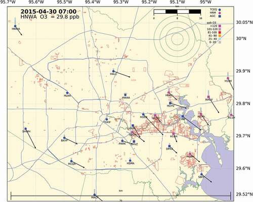
Figure 1. Locations of Texas Commission of Environmental Quality (TCEQ) monitors (blue) and Houston Regional Monitoring (HRM) network sites (magenta) in Houston, TX. Red area outlines are locations of regulated entities. Green lines are county boundaries and blue lines are major roadways. Arrows represent hourly averaged wind speed and direction.

This work aims to identify the most relevant meteorological parameters that can illustrate conditions for high ozone, and could also be applied in a diagnostic model performance evaluation (EPA 2014). A diagnostic evaluation focuses on model processes providing insights on the occurrence of compensating errors. In this work these parameters were developed using more than a decade of observational data that include both regulatory and private monitoring networks. These parameters, and the meteorological conditions they describe, are influenced by large scale synoptic forces whose description are also provided and supported with observational data from across the state of Texas.

Methods

Observational data

Surface measurement data of wind speed, direction, and hourly ozone concentrations were collected from three Texas cities: Houston, San Antonio, and El Paso. In each case, observational data were collected from regulatory Continuous Ambient Monitoring Stations (CAMS) operated by the Texas Commission on Environmental Quality (TCEQ). In Houston, data from all days in 2000–2015 from the TCEQ were used at the locations listed in Supplemental Table 1 and shown as blue symbols in Figure 1. In addition, data from a private monitoring network in Houston were included that is operated by Houston Regional Monitoring (HRM) (HRM 2021) and are shown as magenta symbols in Figure 1. HRM is a voluntary industry-funded technical resource dedicated to performing ambient air monitoring and related special studies to better understand air quality in the Houston area. For this study, HRM provided monitoring data from all days in 2000–2015. Using both the TCEQ regulatory and the HRM monitors, a total of 99,225 site-days of data were processed as shown in Table 1. About 4% of all days had measurements where the 1-hour ozone concentration was equal or greater than 100 ppb. Similar observational data for 2015 were collected from the Camp Bullis monitor in San Antonio shown in Supplemental Figure 2. Measurement data from El Paso was also examined from the University of Texas – El Paso (UTEP) monitor whose location is shown in Supplemental Figure 2. All monitoring concentration data are averaged over one hour.

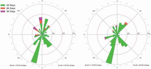
Figure 2. The average 1-hour wind vectors for 2000–2015 at 27 monitors for (left) exceedance days and (right) non-exceedance days. The data is also separated by (top) March to July and (bottom) August to October. An exceedance day is determined if the daily maximum 8-hour ozone concentration is greater to or equal than 70 ppb. Colors indicate the time of day, and each dot is the wind vector tail.

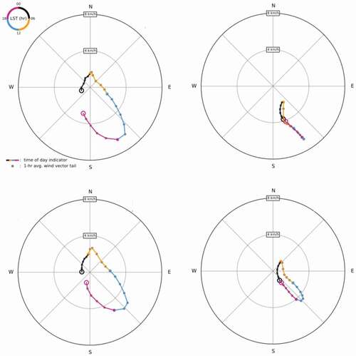
Table 1. Exceedance statistics for observations during 2000–2015 for 21 TCEQ regulatory monitors, and 6 HRM monitors. An exceedance is defined as having a 1-hour O₃ measurement equal or greater than 100 ppb.

	Regulatory (21)	All Monitors (27)
Non-Exceedance (March-July)	46,646	59,792
Non-Exceedance (August-October)	27,303	35,063
TOTAL Non-Exceedance	73,949	94,853
Exceedance (March-July)	1,549	2,173
Exceedance (August-October)	1,677	2,199
TOTAL Exceedance	3,226	4,372
TOTAL	77,175	99,225
Fraction Exceedance Days	4.2	4.4

For this investigation, a comprehensive study was completed on available processed radar wind profiler data from across Texas that covered June 1, 2005 through October 31, 2006. Six of these profilers were part of the 404 MHz National Oceanic and Atmospheric Administration (NOAA) Profiler Network and typically detected winds at 500 to 15,000 m above ground level (AGL) with a vertical resolution of 250 m AGL. The remaining profilers operated at 915 MHz and typically detected winds between 120 m AGL and 4000 m AGL, though data are only reliably available up to 2500 m AGL under typical summertime conditions. The boundary layer profiler data underwent separate quality control, including screening for contamination of velocities by migrating birds (Knoderer and Macdonald 2021).

Mixed layer sea breeze model

A simple model for the trajectory of an air parcel within the planetary boundary layer in response to diurnal temperature changes near a coastline was developed by Daewon Byun, drawing on work by Gutman and Berkofsky (Gutman and Berkofsky 1985) and Byun and Arya (Byun and Arya 1990). Dr. Byun produced a complete formulation of the mixed surface transport which captured key aspects of the observed evolution of winds during high ozone events, but his work was not published before his untimely death in 2011. In this work his model and results are re-created to illustrate the diurnal wind patterns that are associated with ozone exceedances and the combination of factors that cause those patterns to arise. The model expresses the changes in mean mixed layer velocity in terms of the mixed layer height gradient, the horizontal temperature gradient, the Coriolis effect, large-scale winds, and turbulent drag.

In a 2005 presentation (Byun et al. 2005), Dr. Byun combined the mixed layer height and horizontal temperature variations into a single thermal forcing term that drives a horizontal pressure gradient. In a coastal environment, the diurnal thermal forcing is produced by the gradient between relatively constant sea surface temperatures and diurnally changing land temperatures. In the present implementation, the land temperatures are assumed to vary according to an idealized diurnal cycle (Parton and Logan 1981). For simplicity, the resulting pressure gradient is assumed to be horizontally uniform, as are the resulting winds. An additional simplification treats the magnitude of friction as proportional to the wind speed (Byun and Arya 1986). Further details on the equations used in the mixed layer model are provided in the supplementary information.

Results

Daily wind rotation

Since the previous daily wind rotation analysis was limited to 1998–2000, it was expanded in this analysis for 2000–2015 for monitor sites in HGB. In this analysis an exceedance day is defined as the daily maximum 8-hour ozone concentration being greater or equal to 70 ppb. In Houston, the ozone season begins in March and runs until November and the data was limited to that period. These days were further split into the March–July and August–October time periods to see if any variability existed across these periods. Figure 2 shows that the average winds of all exceedance days, 4,372 monitor days, show a direction that traverses the entire compass during a day. These are similar to the 1998–2000 analysis, showing a consistent pattern over many years of observational data (Breitenbach 2001). Exceedance days were similar under both periods. The rotational pattern shown on the exceedance days showed little variability upon close investigations by specific monitor and across all years. In the vast majority of instances an exceedance day had a 0–6 LST wind direction from the W-N quadrant and had a wind direction that traversed all four compass quadrants. The average of all non-exceedance days, 94,853 monitor days, had wind directions that remained relatively steady as one of two common types of flow regimes: wind flows mostly from the north for the entire day, or wind flows mostly from the south. When these two types of days are included in the average, the result is a hodograph wind direction (Figure 2, right side) that reflects neither regime. As shown in later analysis these non-exceedance days typically have higher wind speeds than shown in this average. Thus, these plots are only appropriate for the screening of multi-quadrant days, and any conclusions on wind flow directions should be confirmed with more temporally resolved wind direction data.

Based on these insights, a monitor-by-monitor analyses was completed that used the wind direction data to estimate the number of compass quadrants traversed over a day. For the HGB sites, the wind speed and direction were sorted into the number of daily wind quadrants. These quadrants were further sorted into the number of O₃ non-exceedance and exceedance days and visualized with pie charts. This quadrant analysis provides a simple view of the relationships amongst a 24-hour wind direction and exceedance ozone at a monitor site. This analysis was completed for all years and monitors and the years 2012 and 2015 are featured here. The year 2012 was chosen as it is the base year for modeling used in support of two of the TCEQ’s State Implementation Plans (SIP) submitted in 2016 (TCEQ 2016) and 2020 (TCEQ 2020). The year 2015 was chosen as the most representative of all years analyzed. All monitors data for the years 2012 and 2015 are publicly available (Vizuete 2021a, 2021b).

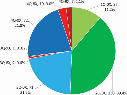
A quadrant analysis is shown for the HO3H monitor in Figure 3 for the entire year of 2015. The location of the HO3H monitor is shown in Figure 1 located east of downtown Houston and just north of the Houston Ship Channel (HSC). In 2015, nearly half the days are characterized with wind directions from one quadrant (1Q) or two quadrants (2Q), with the other half distributed among three-quadrant (3Q) and four-quadrant (4Q) days. Also shown are the number of days for each quadrant with no exceedances (0X), a one-hour (1 h) exceedance (1X) of O3 ≥ 100 ppb, an eight-hour (8 h) average exceedance (8X) of O3 ≥ 70 ppb, or both a 1 h and 8 h exceedance (9X). The most insightful element of this analysis is how rarely exceedance days occur on a 1Q or 2Q day. For example, Figure 3 shows that all exceedances at this monitor are on a 4Q or 3Q day. Further, up to 96% of these 4Q and 3Q days are not in violation of the ozone standard, meaning other conditions are also needed. This even distribution among quadrants remains fairly consistent in the urban core of HGB, but deviates somewhat at the outer monitors. Supplemental Figure 3 shows a quadrant analysis for the MACP and HNWA monitors located further from the urban HGB core (Figure 1). The correlation of exceedances remains strong with the 3Q and 4Q days, however, the distribution of quadrants have changed. For these monitors the number of 1Q days is less and there are more frequent 3Q days.

Figure 3. For the HO3H monitor for 2015 the number of compass quadrants (1Q-4Q) traversed by the wind direction during a 24-hour period. Also shown are the number of days with no exceedances (0X), a one-hour exceedance (1X) ≥ 100 ppb, 8-hour average exceedance (8X) ≥ 70 ppb or has a one-hour and eight-hour exceedance (9X).

Morning wind conditions

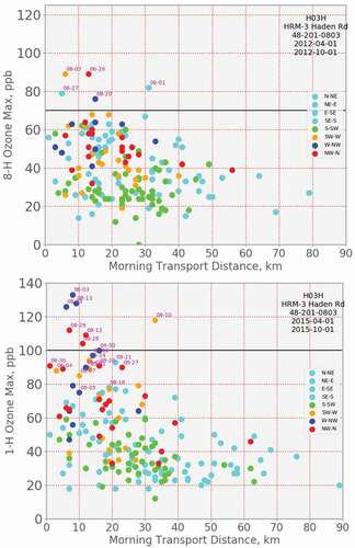
Figure 4 shows, for April to October 2015 at the H03H site, the daily peak ozone levels for 8-hour averaged ozone plotted against the morning transport distance. The morning transport distance is defined as the approximate distance traveled by an air parcel from a monitor starting at midnight and ending six hours later. The hourly wind speeds at the monitor from 0 to 6 LST (morning) were used in this calculation to estimate the total distance that the air parcel would travel in six hours. A color code indicates which compass octant applied to the morning wind. In this analysis, a one-hour exceedance is defined as hourly ozone greater or equal to 100 ppb. As shown in Figure 4, the highest 1 h and 8 h ozone observations had morning transport distances less than 20 km. The rare exception occurred on August 10, 2015, with a 34 km travel distance. Further investigation of this day shows a relatively unchanged wind direction in the morning followed later in the day by a rapid 180° change in direction. This was an extremely rare occurrence as nearly all exceedances had much shorter morning transport distances. Also shown in Figure 4 are the results for April–October 2012 with similar results. Morning transport distance and one-hour averaged ozone concentrations are also found in Supplemental Figure 4 for 2012 and 2015. As shown in these plots there is rarely a one-hour ozone concentration in excess of 100 ppb when morning transport distances are greater than 20 km. These distances suggest that local emission sources could play more of a role in impacting ozone formation during exceedance days.

Figure 4. For the Houston HO3H monitor, during 0–6 LST, the starting wind direction (color) and the morning transport distance versus 8-hour (8-H) averaged ozone concentrations for April 1 – October 1 for (Top) 2012 and (Bottom) 2015.

In addition to the morning wind speed, the wind direction was found to have a strong correlation with an ozone exceedance day. Figure 5 shows, for the HO3H monitor, the midnight wind direction and the number of compass quadrants the wind direction traversed over 24 hours for Apr 01-Oct 01 of 2012 and 2015. Also shown are the number of days for each quadrant with and without an exceedance. Figure 5 shows that in 2015 the majority of the higher observed ozone values came from the W-NW and NW-N wind octants. When compared to 2015 there were fewer exceedances than in 2012. Figure 5 also shows that there were a limited number of exceedance days with morning wind directions from NE to SW, with many of the highest exceedances having directions of NW-N or W-NW. The morning wind speed and direction was found to have a strong correlation with an exceedance for that day.

Figure 5. For the HO3H monitor the midnight wind direction, the number of compass quadrants the wind direction traversed over 24 hours for Apr 01-Oct 01 of (left) 2012 and (right) 2015. Also shown are the number of days for each quadrant with no exceedances (0X), 8-hour average exceedance (8X), or has a one-hour and eight-hour exceedance (9X).

Impacts on ozone

In HGB, the number of wind quadrants occurring on a given day has a clear impact on how much ozone can be produced. This was evident in several case studies where the wind conditions that produced a multi-quadrant day also coincided with high production of ozone. There were other cases, the majority in fact, where similar wind conditions produced far less ozone. This suggests that a multi-quadrant day is a necessary meteorological condition, but that other conditions are needed to produce an ozone exceedance. Figure 6 provides an illustrative case of these conditions using ozone and wind data for May and August of 2012 and 2015 collected at the BAYP monitor. These plots were made for all monitors and the years 2012 and 2015 are publicly available (Vizuete 2021c). Thirty days in May 2012 at the BAYP monitor are shown in the top plot of Figure 6. At the top of the this plot the multicolored lines and dots are the hourly kilometer displacement of flows based on the observed wind speed and direction. It shows the distances to the site using the monitor’s morning wind speeds and directions at the monitor with an air parcel arriving at the monitor at noon. Using the afternoon wind speed and direction the plot shows the trajectory for an air parcel leaving the monitor at noon. Focusing on the early morning wind directions, they start from the south-east at the beginning of the month and then rotate to the north in the middle of the month before returning to the south and east at the end of the month. This rotation of the 0 LST wind directions impacted many of the monitors through HGB and was a common pattern across years. The longer length of the trajectories also coincides with higher wind speeds in the beginning and end of the month as shown in the blue trace. Beside each trajectory is a label showing the number of quadrants traversed during that day. The higher wind speed days with longer trajectories are 1Q and 2Q days. During the middle of the month the wind speeds are slower, trajectories more compact, and the result are more 3Q and 4Q days. The black trace at the bottom of the plot shows elevated ozone concentrations during the middle part of the month.

Figure 6. For the BAYP monitor the displacement, ozone concentration, wind speed and direction for the (top) May 2012 and (bottom) May 16–20, 2012. Black stair-stepped line is the 1-Hour average ozone, and the red horizontal bar is the computed highest 8-Hour average ozone for the day. The blue stepped line is the 1-Hour resultant wind speed arriving at site where the blue text on the right-side y-axis label provides the wind speed. The multicolored lines and dots at top of chart are the hourly kilometer displacement of flowsto and away from the site, and are centered at noon at the site. The colored segments are each 6 hours long, small gray circles mark each hour, and the kilometer scale of displacement is shown in the upper left of plot with a color code for each 6-hour segment. The magenta digit and letter “q,” are the number of wind quadrants occurring in each displacement plot. The black numbers next to 1 h ozone is the annual rank of the 1 h ozone maximum value (only shown for days with ranks 1–60) and the red numbers next to the 8 h ozone is the same for the 8 h ozone maximum value.

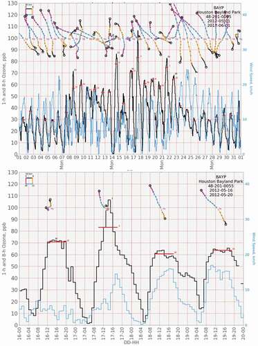
To further illustrate the relationships of quadrants, trajectories, and high ozone during this month, Figure 6 shows data collected during a key period from May 16–20, 2012. May 16 and 17 are both 4Q days and have compact trajectories indicative of lower wind speeds and thus more conducive for producing ozone. On the other hand, May 18 and 19 had higher wind speeds, resulting in more elongated trajectories and lower ozone concentrations. Only with the trajectories found on a 4Q day were the conditions ideal for ozone production, and on May 17 the monitor recorded the third highest eight-hour ozone concentration of the year. It is important to note that May 16 also had similar meteorological conditions, but produced less ozone than was observed on May 17. It is also possible that the slower wind speeds on May 16^th, and the resultant chemical oxidation, may have also contributed to the ozone exceedance on May 17^th. Both days had the necessary meteorological conditions, but only the 17^th had the additional sufficient conditions needed for an exceedance. Many of the 4Q day trajectories with ozone exceedances intersected the HSC. Previous studies of this area have shown that some observed localized exceedances of ozone were the result of episodic emissions of volatile organic carbons (VOCs) (Henderson et al. 2010; Murphy and Allen 2005; Nam et al. 2006). Ambient observations, and industrial process data from the HSC, have also shown the occurrence of episodic emissions of VOCs from flares (Nam et al. 2008; Pavlovic et al. 2012). The episodic nature of these emissions suggests that further investigations should focus on the possible continued presence of episodic emission VOC events from the HSC.

Previous studies have shown that when meteorological conditions are conducive for high ozone, there is also a larger number of low ozone days. For example, a study using five-month ozone periods (May–September) in 2005 and 2006 found two meteorological clusters where high-ozone events happened more frequently (Ngan and Byun 2011). Only half of the total days (44% and 48%), however, had a recorded eight-hour average ozone level that exceeded the Environmental Protection Agency (EPA) standard for these clusters. In the Davis et al. 1998 study, the cluster that included the maximum ozone concentrations also included days where the maximum ozone concentrations were as low as 40 ppb (Davis et al. 1998). The lack of a strong correlation between high ozone and meteorological conditions is also seen in more recent Houston analyses. Using the National Centers for Environmental Prediction (NCEP) data for the summers of 2000 through 2014, with a nonhierarchical K-means unsupervised partitioning method, researchers identified seven meteorological clusters (Souri et al. 2016). These results confirmed previous studies that associated high ozone days with weak easterlies and low ozone days with higher wind speeds. These researchers also reported that even in the cluster classified as having the highest ozone days, only 26% of these days had eight-hour ozone exceedances. Even the applications of more complex non-Gaussian statistical models have difficulties predicting high ozone days in HGB. Using a generalized linear mixed-effects model, researchers calculated a True Positive Rate (TPR) for a regulatory monitor in Deer Park monitor as low as 17% (Sun et al. 2015).

Observations across Texas

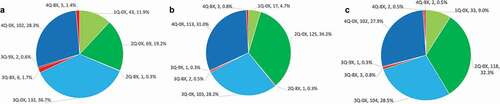
The analysis of the HGB data provides the basis for the use of observational based parameters to investigate if similar patterns can be found across the state. A quadrant analysis for 2015 is shown in Figure 7 for San Antonio’s BULL site and for El Paso’s UTEP site. Like the Houston monitors, these sites also experience 1Q-4Q days throughout the year. For reference the HGB HNWA monitor is also shown in Figure 7 for the same year. Although in a different part of the state, the distributions of quadrants days are similar for all three sites. In San Antonio and El Paso, the highest percentage of O₃ exceedances that occurred on 2Q days has been <0.3%. These 2Q trajectories show essentially a 1 h complete 180° reversal of flow back over the prior trajectory path. These may be associated with diurnally driven upslope and downslope flow reversals under light ambient wind conditions, circumstances that would be most likely to occur in El Paso. In all three cities, no O₃ exceedances have been observed at monitors under 1Q conditions.

Figure 7. The (A) San Antonio Camp Bullis, (B) El Paso UTEP, and (C) HGB HNWA monitors for 2015 with the number of compass quadrants (1Q-4Q) traversed by the wind direction during a 24-hour period. Also shown are the percentage and number of days for each quadrant. Also shown are whether there are no exceedances (0X), 8-hour average exceedance (8X), or a one-hour and eight-hour exceedance (9X).

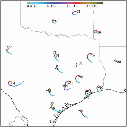
Other measurement data also supports similar wind profiles across the state of Texas. Figure 8 shows the resulting composite 500 m AGL trajectories based on filtered wind profiler data. Trajectories are based on winds measured locally by each profiler over 24-hour periods ending at 6 LST and are drawn with the endpoint at the profiler location. Each composite trajectory is based on the average of hourly winds during all warm-season (May–October) days with sufficiently complete data in which the vector mean wind speed over the 24-hour period was less than 3 m/s. The number of such days is plotted next to each profiler location. Trajectory timing is indicated by the legend at the top of the figure. It is clear from Figure 8 that light winds favor four-quadrant days across the entire region.

Figure 8. Composites of light-wind trajectories at 500 m from radar wind profilers operating in Texas in May–October 2005 and 2006. Each trajectory lasts 24 hours and is assumed to terminate at the profiler site at 1800 LST (0000 UTC). Colors indicate time of trajectory segments, and numbers indicate total number of wind days included in the composite for each profiler. To be included, the day’s resultant wind speed must be less than 3 m/s.

As discussed above, the wind rotation near the coast has been associated with an inertially dominated land-sea breeze circulation response. Similar wind patterns much farther from the coast indicate that inertial rotation of winds in Texas do not require sea breeze forcing. Under strong wind conditions, the Great Plains low-level jet nocturnal wind maximum in Texas and elsewhere involves an inertial response to diurnally varying vertical mixing, but the inertial rotation shown here inland under light wind conditions is unexpected and will require further investigation.

Mixed layer sea breeze model

A simple mixed layer sea breeze model is used here to illustrate how and why wind rotation and the existence or nonexistence of stagnation can be dependent on large-scale and local conditions. This model is able to reproduce the basic patterns produced by the diurnal temperature cycle and reacts appropriately to differences in background winds, defined as the winds associated with large-scale pressure gradients as modified by surface friction. Figure 9 shows the model trajectories that result from typical conditions in Houston in the summer. Specified parameters include temperature, wind speed and direction, coastal orientation, and boundary layer height.

Figure 9. One-day modeled mixed-layer wind trajectories with varying background wind strengths. Winds are modeled with a straight coastline oriented similar to Houston, TX. Numbers along the trajectories indicate hours after trajectory starting point: 0 = 18:00 LST; 6 = Midnight LST; 12 = 0600 LST the next day; 18 = Noon LST the next day; 24 = 18:00 LST the next day.

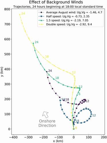
These parameters produce trajectories that are very similar to those shown in Figure 8, resembling the composite trajectories observed in 2005–2006. For example, the composite trajectory in Figure 8 for LaPorte, near Houston, and the model-simulated trajectory in Figure 9 for average August winds (dark blue) both feature strong onshore flow during the evening hours, clockwise rotation and decreasing wind speed overnight, minimum wind speeds from the northwest in the early morning, and acceleration of winds toward the west and northwest during the afternoon. While the overall trajectory shapes are quite similar, the observed wind variations appear to lag the model-simulated wind variations by about three hours. Locations farther inland have similar observed trajectory shapes but the timing of their features lags the idealized trajectory even more. This discrepancy between model and observed timing is interpreted as the effect of gravity waves, as the diurnal pressure variation generated at the coastline propagates inland (Rotunno 1983). The idealized model applies at the coastline itself and does not explicitly incorporate the time required for the sea breeze signal to propagate inland. Allowing for the difference in phase inland of the diurnally-varying pressure gradient, though, the model still illustrates the resulting trajectory shapes.

Another difference between model and observations is found when considering the stagnation events seen in surface winds. In the model, even wind speeds half of the summertime average do not produce the transport distances of less than 20 km from 0 to 6 LST as shown in Figure 4. This is in part because the model is simulating winds averaged through the roughly 1 km depth of the boundary layer, while the observed trajectories in Figures 2 and 6 are within 10 m of the ground where friction and low-level obstacles reduce wind speed and total apparent transport distance.

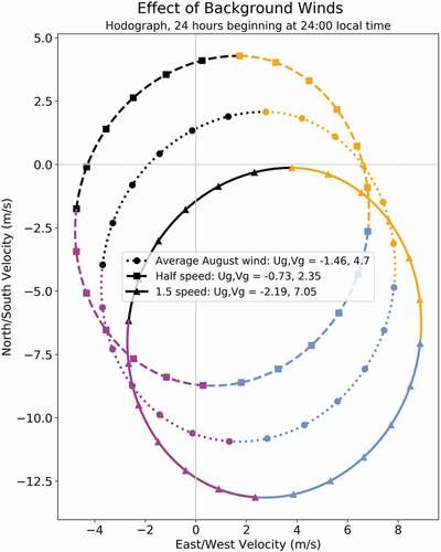
Different values of background winds change the trajectories in two important ways. Wind trajectories are elongated in the direction of the background flow, and stronger winds are associated with smaller loops. With sufficiently strong winds, or sufficiently weak sea breeze variations, the loops disappear completely. The corresponding hodographs show that the wind vectors trace complete circles even in strong wind conditions, but the overall wind direction remains primarily from the southeast because the background wind overwhelms the sea breeze rotation (Figure 10).

Figure 10. Modeled mixed-layer wind hodographs with varying background wind strengths. Colors indicate time of day as in Figure 2. Hodograph is drawn with wind vector tails (originating) along the circles and wind vector heads (terminating) at 0,0. Negative velocities correspond to winds from the south and/or west. All hodographs are circular, but only the average and half-speed hodographs encircle the origin and thus produce winds that perform a complete rotation.

The mixed layer sea breeze model also illustrates how the wind behavior from midnight to 6 AM relates to the number of quadrants the wind direction traverses in one day (Figure 11). With background large-scale winds from the southeast, a midnight wind direction observed from the northwest implies that air parcels are in the process of executing a complete loop. Stronger background winds decrease the probability of having local northwest winds at midnight, and thus the probability of 4Q winds over the course of the following day.

Figure 11. The effect of background winds on the number of quadrants that modeled winds traverse in a day. Arrows represent wind vectors at each hour of the day, colors indicate individual compass quadrants. The top subplot is with no background winds. The subplots below it shows modeled winds using the climatological average for mean boundary-layer winds over Houston in August (u = −1.46 m/s, v = 4.70 m/s) at 100%, 150%, and 200% of average speed.

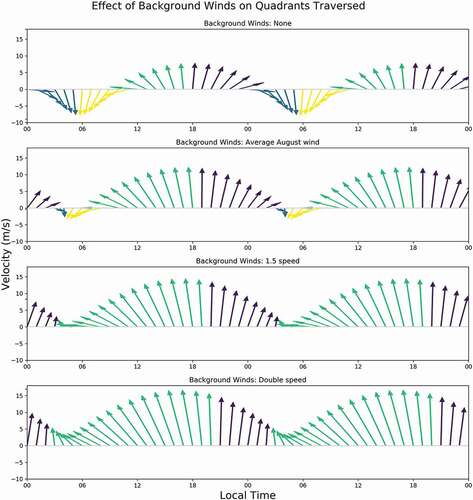
These wind patterns arise because of the Coriolis force and the diurnally changing horizontal temperature gradient at the coast. The Coriolis force is an apparent force caused by the rotation of the Earth. In the Northern Hemisphere, in the absence of other forces it would cause wind directions to rotate steadily clockwise at a rate dependent on latitude. At Houston’s latitude, near 30 degrees, a complete 360-degree rotation (an “inertial oscillation”) would take 24 hours. This is resonant with the diurnal forcing produced by coastal temperature contrasts and boundary layer growth and decay. In the presence of a large-scale background wind any rotation triggered by an imbalance, such as a rapidly changing coastal pressure gradient, will still induce the tip of the full wind vector to trace a circle over 24 hours (Figure 10). The total wind direction variation, however, will be much smaller. In the mixed layer sea breeze model, the circles are similar size under light and strong wind conditions, but in the real world the coast-driven inertial oscillation would be expected to be smaller because air parcels spend less time residing in the coastal zone.

Conclusion

This study provides observational-based parameters developed using 15 years of ozone concentrations and localized wind conditions that described the most common meteorological conditions for an exceedance day. It was found that the six hours after midnight are a critical window for setting up high ozone production that leads to an exceedance in the afternoon. These days also feature a wind direction that rotates clockwise, traversing all four compass quadrants in a 24-hour period. These meteorological conditions are the result of the interaction of the background pressure gradient and Coriolis forces in the presence of diurnal coastal thermal forcing and can be stimulated with a mixed layer sea breeze model. This interaction, and resulting daily wind rotation, can also be observed throughout the state of Texas, including in monitor data from the cities of San Antonio and El Paso. These data suggest that inertial rotation of winds found inland do not require sea breeze forcing and is an area for future work.

To assess regulatory model performance the EPA developed a model performance evaluation (MPE) framework (EPA 2014) whose minimum requirement for an attainment demonstration is an operational evaluation using all available ambient monitoring data for the model simulation period. Operational evaluations, however, provide insufficient evidence to conclude whether an AQM’s “good” performance was the result of accurate science, or the product of compensating errors. For this reason, the MPE framework recommends completing a diagnostic evaluation that focuses on processes that determine the final concentrations providing insights on whether the model processes are producing the predicted concentration for the right reason. For these cities in Texas, the focus on rotational winds and the timing of low wind speeds could be added as part of a diagnostic analysis within the MPE framework. A model that sufficiently passes an operational evaluation, but is unable to reproduce the observed timing or degree of rotation of winds could suffer from compensating errors. Thus, an anlaysis such as described here could be used in support of regulatory model performance evaluations in Texas to assure accuracy in developing effective mitigation.

The vast majority of days used in this study, however, do not produce exceedance levels of ozone concentrations. This suggests that this meteorology is necessary, but some combination of other conditions is also necessary to produce an exceedance. The infrequency of high ozone days suggests that additional intermittent conditions, such as variable emission sources of a precursor, or high background ozone levels are likely needed. Furthermore, the observed ozone plume appears to not extend over a large spatial region since it only impacts a few monitors at a time. The short morning transport distances, and the location of origin of the ozone plumes, suggest sources that could be found in the industrial Houston Ship Channel. Although the ample emissions of NO_x found in the HGB are necessary to produce these ozone plumes, it is difficult to imagine a scenario in which variable NO_x emission source alone would create a relatively localized ozone plume. The Houston Ship Channel has historically been the source of episodic VOC emissions and follow-up analysis will focus on investigations of sources and activities (Henderson et al. 2010; Murphy and Allen 2005; Nam et al. 2006, 2008; Pavlovic et al. 2012). Further analysis will also consider the possible long-term influence of changing emission strengths from other sectors and deviations in meteorological parameters due to a changing climate.

Acknowledgment

This work would not have been possible without the generous guidance, wisdom, and years of tireless service provided by Dr. Harvey Jeffries. The authors also express gratitude to the anonymous reviewers and to the cooperation and guidance from the Texas Commission on Environmental Quality and the Houston Regional Monitoring Network.

Disclosure statement

No potential conflict of interest was reported by the author(s).

Data availability statement

The data that support the findings of this study are openly available in UNC Dataverse at 10.15139/S3/BP5B95, 10.15139/S3/7DNRJP and 10.15139/S3/YAVDSI.

Supplementary material

Supplemental data for this paper can be accessed on the publisher’s website

Additional information

Notes on contributors

William Vizuete

William Vizuete is an Associate Professor in the Department of Environmental Sciences and Engineering (ESE) at the University of North Carolina at Chapel Hill (UNC). Tackling the problems of air pollution mortality and climate change are the global public health issues that motivate Dr. Vizuete’s research. In his research he focuses on understanding how the atmosphere can change the formation processes of ozone and particulate matter (PM), and its connection to human health. Through his research Dr. Vizuete has increased our scientific knowledge in these areas and produced new insights through air quality models, field studies, laboratory experiments, and the development of a novel in vitro technology. https://vizuete.web.unc.edu

References

- Banta, R. M., C. J. Senff, R. J. Alvarez, A. O. Langford, D. D. Parrish, M. K. Trainer, L. S. Darby, R. M. Hardesty, B. Lambeth, J. A. Neuman, et al. 2011. Dependence of daily peak O-3 concentrations near Houston, Texas on environmental factors: Wind speed, temperature, and boundary-layer depth. Atmos. Environ. 45 (1):162–73. doi:10.1016/j.atmosenv.2010.09.030.
- Banta, R. M., C. J. Seniff, J. Nielsen-Gammon, L. S. Darby, T. B. Ryerson, R. J. Alvarez, S. R. Sandberg, E. J. Williams, and M. Trainer. 2005. A bad air day in Houston. Bull. Am. Meteorol. Soc. 86 (5):657. doi:10.1175/BAMS-86-5-657.
- Berlin, S. R., A. O. Langford, M. Estes, M. Dong, and D. D. Parrish. 2013. Magnitude, decadal changes, and impact of regional background ozone transported into the greater Houston, Texas, Area. Environ. Sci. Technol. 47 (24):13985–92. doi:10.1021/es4037644.
- Bernier, C., Y. Wang, M. Estes, R. Lei, B. Jia, S. C. Wang, and J. Sun. 2019. Clustering surface ozone diurnal cycles to understand the impact of circulation patterns in Houston. TX. J. Geophys. Res.: Atmos. 124 (23):13457–74. doi:10.1029/2019JD031725.
- Blanchard, C. L., F. W. Lurmann, P. M. Roth, H. E. Jeffries, and M. Korc. 1999. The use of ambient data to corroborate analyses of ozone control strategies. Atmos. Environ. 33 (3):369–81. doi:10.1016/S1352-2310(98)00223-4.
- Breitenbach, P. 2001. Meteorological model for Houston/Galveston ozone events. Science Team Meeting. Austin, TX: TCEQ.
- Byun, D.-W., and S. Arya. 1986. A study of mixed-layer momentum evolution. Atmos. Environ. 20 (4):715–28. doi:10.1016/0004-6981(86)90186-1.
- Byun, D., and S. Arya. 1990. A two-dimensional mesoscale numerical model of an urban mixed layer—I. Model formulation, surface energy budget, and mixed layer dynamics. Atmos. Environ.Part A. General Topics 24 (4):829–44. doi:10.1016/0960-1686(90)90284-T.
- Byun, D., S. Kim, F. Ngan, S. Kim, and B. Cheng, Air trajectory tools and theoretical analysis of the Houston-Galveston Area Land/Sea Breeze, in TexAQS II Intensive Field Study Meeting. 2005: Austin, TX.
- Caicedo, V., B. Rappenglueck, G. Cuchiara, J. Flynn, R. Ferrare, A. Scarino, T. Berkoff, C. Senff, A. Langford, and B. Lefer. 2019. Bay breeze and sea breeze circulation impacts on the planetary boundary layer and air quality from an observed and modeled DISCOVER‐AQ Texas case study. J. Geophys. Res.: Atmos. 124 (13):7359–78.
- Choi, Y., and A. H. Souri. 2015. Chemical condition and surface ozone in large cities of Texas during the last decade: Observational evidence from OMI, CAMS, and model analysis. Vol. 168, 90–101. Elsevier
- Darby, L. S. 2005. Cluster analysis of surface winds in Houston, Texas, and the impact of wind patterns on ozone. J. Appl. Meteorol. 44 (12):1788–806. doi:10.1175/JAM2320.1.
- Davis, J. M., B. K. Eder, D. Nychka, and Q. Yang. 1998. Modeling the effects of meteorology on ozone in Houston using cluster analysis and generalized additive models. Atmos. Environ. 32 (14):2505–20. doi:10.1016/S1352-2310(98)00008-9.
- Edwards, R. P., O. Sale, and G. A. Morris. 2018. Evaluation of El Niño-Southern oscillation influence on 30 years of tropospheric ozone concentrations in Houston. Atmos. Environ. 192:72–83. doi:10.1016/j.atmosenv.2018.08.032.
- EPA. 2014. Modeling guidance for demonstrating attainment of air quality goals for ozone, PM2.5, and regional haze, Editor. U. S. E. P. Agency, NC: Research Triangle Park, https://www.epa.gov/sites/production/files/2020-10/documents/draft-o3-pm-rh-modeling_guidance-2014.pdf
- Ge, S., S. Wang, Q. Xu, and T. Ho. 2021. Characterization and sensitivity analysis on ozone pollution over the Beaumont-Port Arthur Area in Texas of USA through source apportionment technologies. Vol. 247, 105249. Elsevier.
- Gorai, A. K., F. Tuluri, P. B. Tchounwou, and S. Ambinakudige. 2015. Influence of local meteorology and NO2 conditions on ground-level ozone concentrations in the eastern part of Texas, USA. Air Qual Atmos Health 8 (1):81–96.
- Gutman, L. N., and L. Berkofsky. 1985. On the theory of the well-mixed layer containing a zero-order jump. Boundary-layer Meteorology. 31 (3):287–301.
- Henderson, B. H., H. E. Jeffries, B.-U. Kim, and W. G. Vizuete. 2010. The influence of model resolution on ozone in industrial volatile organic compound plumes. J. Air Waste Manage. Assoc. 60 (9):1105–17. doi:10.3155/1047-3289.60.9.1105.
- HRM. Houston Regional Monitoring Corporation. 2021 [ cited 2020; Available from: http://hrm.aecom.com
- Knoderer, C. A., and C. P. Macdonald. 2021. TexAQS-II radar wind profiler, radio acoustic sounding system, sodar, and lidar data quality control and mixing height derivation final report STI-907100-3215-FR. Sonoma Technology, Inc. https://www.tceq.texas.gov/assets/public/implementation/air/am/contracts/reports/mm/582564593FY0720_STI_ProfilerQC_Mixing_Final_Report.pdf
- Lei, R., R. Talbot, Y. Wang, S.-C. Wang, and M. Estes. 2018. Influence of cold fronts on variability of daily surface O3 over the Houston-Galveston-Brazoria area in Texas USA during 2003–2016. Atmos. 9 (5):159. doi:10.3390/atmos9050159.
- Li, W., Y. Wang, C. Bernier, and M. Estes. 2020. Identification of sea breeze recirculation and its effects on ozone in Houston, TX, during DISCOVER‐AQ 2013. J. Geophys. Res. Atmos. 125: e2020JD033165.
- Liu, L., R. Talbot, and X. Lan. 2015. Influence of climate change and meteorological factors on houston’s air pollution: Ozone a case study. Atmos. 6 (5):623–40. doi:10.3390/atmos6050623.
- Mazzuca, G. M., K. E. Pickering, R. D. Clark, C. P. Loughner, A. Fried, D. C. S. Zweers, A. J. Weinheimer, and R. R. Dickerson. 2017. Use of tethersonde and aircraft profiles to study the impact of mesoscale and microscale meteorology on air quality. Vol. 149, 55–69. Elsevier.
- Murphy, C. F., and D. T. Allen. 2005. Hydrocarbon emissions from industrial release events in the Houston- Galveston area and their impact on ozone formation. Atmos. Environ. 39 (21):3785–98. doi:10.1016/j.atmosenv.2005.02.051.
- Nam, J., Y. Kimura, W. Vizuete, C. Murphy, and D. T. Allen. 2006. Modeling the impacts of emission events on ozone formation in Houston, Texas. Atmos. Environ. 40 (28):5329–41. doi:10.1016/j.atmosenv.2006.05.002.
- Nam, J., M. Webster, Y. Kimura, H. Jeffries, W. Vizuete, and D. T. Allen. 2008. Reductions in ozone concentrations due to controls on variability in industrial flare emissions in Houston, Texas. Atmos. Environ. 42 (18):4198–211. doi:10.1016/j.atmosenv.2008.01.035.
- Ngan, F., and D. Byun. 2011. Classification of weather patterns and associated trajectories of high-ozone episodes in the Houston-Galveston-Brazoria area during the 2005/06 TexAQS-II. J. Appl. Meteorol. Climatol. 50 (3):485–99. doi:10.1175/2010JAMC2483.1.
- Nielsen-Gammon, J., J. Tobin, and A. McNeel. 2005. A conceptual model for eight-hour ozone exceedances in Houston, Texas Part II: Eight-hour ozone exceedances in the Houston-Galveston metropolitan area.
- Nielsen-Gammon, J., J. Tobin, A. McNeel, and G. Li. 2005. A conceptual model for eight-hour ozone exceedances in Houston, Texas Part I: Background ozone levels in eastern Texas.
- Parton, W. J., and J. A. Logan. 1981. A model for diurnal variation in soil and air temperature. Vol. 23, 205–16. Elsevier.
- Pavlovic, R. T., F. M. Al-Fadhli, Y. Kimura, D. T. Allen, and E. C. McDonald-Buller. 2012. Impacts of emission variability and flare combustion efficiency on ozone formation in the Houston-Galveston-Brazoria Area. Ind Eng Chem Res. 51 (39):12593–99. doi:10.1021/ie203052w.
- Rappengluck, B., R. Perna, S. Zhong, and G. A. Morris. 2008. An analysis of the vertical structure of the atmosphere and the upper-level meteorology and their impact on surface ozone levels in Houston. Texas. J. Geophys. Res, [Atmos.] 113 (D17):D17315. doi:10.1029/2007JD009745.
- Reitze, A. W., Jr. 2015. The national ambient air quality standards for Ozone. Ariz. J. Envtl. L. & Pol’y 6:420.
- Rotunno, R. 1983. On the linear theory of the land and sea breeze. J. Atmos. Sci. 40 (8):1999–2009. doi:10.1175/1520-0469(1983)040<1999:OTLTOT>2.0.CO;2.
- Souri, A. H., Y. Choi, X. Li, A. Kotsakis, and X. Jiang. 2016. A 15-year Climatology of wind pattern impacts on surface ozone in Houston. Texas.Atmos. Res. 174:124–34. doi:10.1016/j.atmosres.2016.02.007.
- Sun, W., A. Palazoglu, A. Singh, H. Zhang, Q. Wang, Z. M. Zhao, and D. Cao. 2015. Prediction of surface ozone episodes using clusters based generalized linear mixed effects models in Houston-Galveston-Brazoria area. Texas. Atmos. Pollut. Res. 6 (2):245–53. doi:10.5094/APR.2015.029.
- TCEQ. 2016. Houston-galveston brazoria attainment demonstration state implementation plan revision for the 2008 eight hour ozone standard nonattainment area. Austin, TX: Texas Commission on Environmental Quality (TCEQ).
- TCEQ. 2020. Houston-Galveston Brazoria serious classification attainment demonstration state implementation plan revision for the 2008 eight-hour ozone national ambient air quality standard. Austin, TX: Texas Commission on Environmental Quality (TCEQ).
- Tucker, S. C., R. M. Banta, A. O. Langford, C. J. Senff, W. A. Brewer, E. J. Williams, B. M. Lerner, H. D. Osthoff, and R. M. Hardesty. 2010. Relationships of coastal nocturnal boundary layer winds and turbulence to Houston ozone concentrations during TexAQS 2006. J. Geophys. Res.: Atmos. 115 (D10). doi:10.1029/2009JD013169.
- U.S. Environmental Protection Agency. 2015. Regulatory impact analysis of the final revisions to the national ambient air quality standards for ground-level ozone. NC, USA: Research Triangle Park.
- Vizuete, W. 2021a. Empirical relationships among wind conditions and ozone exceedances in Houston and other cities in Texas: Quadrant data. Dataverse. V1. doi:10.15139/S3/BP5B95.
- Vizuete, W. 2021b. Empirical relationships among wind conditions and ozone exceedances in Houston and other cities in Texas: Transport distance data. Dataverse. V1. doi:10.15139/S3/7DNRJP.
- Vizuete, W. 2021c. Empirical relationships among wind conditions and ozone exceedances in Houston and other cities in Texas: Trajectory data. Dataverse. V1. doi:10.15139/S3/YAVDSI.
- Wang, Y., B. Jia, W. Sing-Chun, M. Estes, L. Shen, and Y. Xie. 2016. Influence of the Bermuda High on interannual variability of summertime ozone in the Houston-Galveston-Brazoria region. Atmos. Chem. Phys. 16 (23):15265. doi:10.5194/acp-16-15265-2016.