PM_2.5 in Carlsbad Caverns National Park: Composition, sources, and visibility impacts

ABSTRACT

Carlsbad Caverns National Park in southeastern New Mexico is adjacent to the Permian Basin, one of the most productive oil and gas regions in the country. The 2019 Carlsbad Caverns Air Quality Study (CarCavAQS) was designed to examine the influence of regional sources, including urban emissions, oil and gas development, wildfires, and soil dust on air quality in the park. Field measurements of aerosols, trace gases, and deposition were conducted from 25 July through 5 September 2019. Here, we focus on observations of fine particles and key trace gas precursors to understand the important contributing species and their sources and associated impacts on haze. Key gases measured included aerosol precursors, nitric acid and ammonia, and oil and gas tracer, methane. High-time resolution (6-min) PM_2.5 mass ranged up to 31.8 µg m⁻³, with an average of 7.67 µg m⁻³. The main inorganic ion contributors were sulfate (avg 1.3 µg m⁻³), ammonium (0.30 µg m⁻³), calcium (Ca²⁺) (0.22 µg m⁻³), nitrate (0.16 µg m⁻³), and sodium (0.057 µg m⁻³). The WSOC concentration averaged 1.2 µg C m⁻³. Sharp spikes were observed in Ca²⁺, consistent with local dust generation and transport. Ion balance analysis and abundant nitric acid suggest PM_2.5 nitrate often reflected reaction between nitric acid and sea salt, forming sodium nitrate, and between nitric acid and soil dust containing calcium carbonate, forming calcium nitrate. Sulfate and soil dust are the major contributors to modeled light extinction in the 24-hr average daily IMPROVE observations. Higher time resolution data revealed a maximum 1-hr extinction value of 90 Mm⁻¹ (excluding coarse aerosol) and included periods of significant light extinction from BC as well as sulfate and soil dust. Residence time analysis indicated enrichment of sulfate, BC, and methane during periods of transport from the southeast, the direction of greatest abundance of oil and gas development.

Implications: Rapid development of U.S. oil and gas resources raises concerns about potential impacts on air quality in National Parks. Measurements in Carlsbad Caverns National Park provide new insight into impacts of unconventional oil and gas development and other sources on visual air quality in the park. Major contributors to visibility impairment include sulfate, soil dust (often reacted with nitric acid), and black carbon. The worst periods of visibility and highest concentrations of many aerosol components were observed during transport from the southeast, a region of dense Permian Basin oil and gas development.

View correction statement:

Correction

Introduction

The development of unconventional oil and natural gas extraction techniques, including horizontal drilling and hydraulic fracturing, has unlocked significant new U.S. oil and natural gas (O/G) resources and led to a large increase in production from shale and tight oil and gas resources since 2000 (Brown, Lewis, and Weinberger 2015). Shale gas resources can be found in almost 30 U.S. states (U.S. EIA, 2021a). Tight oil production is driving U.S. oil production growth. The two main source regions are the Bakken shale play in the Northern Great Plains and the Wolfcamp shale play in the Permian Basin, located in west Texas and southeast New Mexico (United States Energy Information Administration (EIA) 2021a). Emissions of volatile organic compounds (VOCs) and nitrogen oxides (NO_x) from oil and gas (O/G) operations have received attention due, in part, to their impacts on the production of ozone (Brown, Lewis, and Weinberger 2015; Field et al. 2015; Hecobian et al. 2019; Olaguer 2012; Prenni et al. 2016; Thompson, Hueber, and Helmig 2014). Less attention has been paid to the effects of O/G activities on particle concentrations and regional haze.

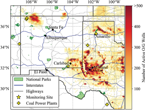
In this study, we examine the impact of O/G development and other sources on air quality in Carlsbad Caverns National Park (CAVE) in 2019. The park is located near extensive oil and natural gas development in the Permian Basin (Figure 1). The major formation in this region is the Wolfcamp shale play (Gaswirth et al., 2018). This region is responsible for much of the shale gas production growth in the United States (U.S. EIA, 2021b). CAVE is in Eddy County, New Mexico, where 77% of SO₂ and 56% of NO_x emissions in the 2017 NEI are from petroleum and related industries. The next largest contributor is industrial fuel combustion for both SO₂ and NO_x, accounting for 17% and 23%, respectively. In neighboring counties (Lea NM, Culberson TX, Loving TX, and Reeves TX) to the south and east, an important upwind transport region during the study, petroleum and related industries accounted for 88% of SO₂ emissions and 71% of NO_x emissions (U.S. EPA, 2019). CAVE and the nearby town of Carlsbad frequently record high ozone values, often exceeding the 8-hr-average 70 ppbv National Ambient Air Quality Standard. A prior screening study of national parks in the southwestern U.S. (Benedict et al. 2020) revealed significant impacts of O/G emissions on VOC levels in CAVE, especially for light alkanes. The 2019 study in CAVE was motivated by these high ozone and VOC levels, along with concerns over sources of fine particle haze, and potential connection to a variety of regional sources including urban emissions, increased O/G development, wildfires, and erosion. Here, we focus primarily on aerosol concentrations in the park, their contributions to regional haze, and their sources. CAVE ozone and VOC levels will be discussed in a future publication.

Figure 1. Active oil and natural gas wells near Carlsbad Caverns National Park (CAVE) (HIFLD, 2019). The color bar gives the number of active O/G wells in the given grid cell. The grid cell resolution is 0.1 degree by 0.1 degree. Cells with 500 or more active wells are shown with the same color. National Park boundaries are shown in green. Larger cities in the surrounding area are marked with black dots and labeled. The monitoring site, in CAVE is shown as a yellow star. Coal-fired power plants in the region are shown as yellow plus signs (U.S. EIA, 2022).

O/G operations and associated traffic and infrastructure can lead to direct emission of fine particulate matter (PM_2.5) and of gaseous precursors that lead to secondary particle formation. Black carbon (BC) is emitted from incomplete combustion processes and is associated with O/G development and production, with emissions from flaring and diesel engine use (Bond et al. 2006; Khalek et al. 2015; Shen et al. 2021; Yanowitz, McCormick, and Graboski 2000). During flaring excess gas is burned and can yield significant emissions of NO_x, BC, and methane (CH₄) during incomplete combustion (Allen et al. 2016; Böttcher et al. 2021; Conrad and Johnson 2019; Weyant et al. 2016). BC is of particular interest because of its strong absorption of solar radiation, in addition to the general adverse health impacts of PM_2.5 (Bond et al., 2013). Other organic aerosol species can also be emitted or formed by secondary processes/reactions producing secondary organic aerosol (Pandis and Seinfeld 2016).

Oil and gas development and production can also impact levels of sulfate, nitrate, and ammonium particulate species. Direct emission of sulfur dioxide (SO₂) and NO_x leads to the formation of sulfuric and nitric acids, respectively. Both can react with ammonia (NH₃) to form hygroscopic particles with important implications for total PM and light scattering. Ammonium nitrate formation, in particular, has been tied to O/G operations in the western U.S. (Elvidge et al. 2009; Evanoski-Cole et al. 2017; Li et al. 2012; Prenni et al. 2016). The formation of ammonium sulfate ((NH₄)₂SO₄) and ammonium nitrate (NH₄NO₃) is dependent on ammonia availability and thermodynamic conditions. If ammonia is very limited, sulfuric acid will exist in the particle phase. As ammonia availability increases, NH₄HSO₄ (ammonium bisulfate), (NH₄)₃H(SO₄)₂ (letovicite), and (NH₄)₂SO₄ (ammonium sulfate) can form. Once the sulfate has been neutralized, ammonium nitrate may form (Pandis and Seinfeld 2016); this is favored at lower temperatures and higher relative humidities (Krueger et al. 2003) and when gaseous nitric acid (HNO₃) and ammonia (NH₃) are abundant. Nitric acid can also react with sodium chloride from sea salt particles and calcium carbonate in the soil.

Many national parks and wilderness areas, collectively known as Class I areas, are protected from visibility degradation by the Clean Air Act and Regional Haze Rule (RHR) (U.S. EPA, 1999). Since 1985, the Interagency Monitoring of Protected Visual Environments (IMPROVE) network has collected extensive long-term monitoring data in these visually protected environments. Visibility degradation results from absorption and scattering of light by particle and gas-phase species in the air, typically expressed through a light extinction coefficient (b_ext). With considerable U.S. O/G development occurring close to national parks and other visually protected environments, there is concern that O/G activities could adversely affect air quality in these sensitive environments and hinder progress toward further reductions in regional haze.

Methods

Measurement site

The Carlsbad Caverns Air Quality Study (CarCavAQS) was conducted at CAVE in southeastern New Mexico from July 25 to September 5, 2019. Measurements were made at the CAVE Biology Office and building 58 (32.18° N, 104.44° W), located within the park, ~0.5 km from the park visitor center. The altitude of the site was approximately 1,355 m. Of the measurements discussed below, University Research Glassware (URG) denuder/filter pack inlets were set at approximately 1 meter above ground level (agl), and all other instrument inlets sampled from approximately 6-m agl. Meteorological data were collected at the same site location, using the meteorological station 35-015-0010, operated by the National Park Service (data can be found at: https://ard-request.air-resource.com/data.aspx).

Measurements

Measurements of meteorological conditions, VOCs, ozone, PM_2.5, other gas species, and nitrogen deposition were collected at different sampling integration periods. Here, our focus is primarily on the characterization of aerosol mass and composition, along with concentrations of key trace gas species important either as aerosol precursors or as source indicators. The measurements used in this work and associated time resolutions are shown in Table 1. The IMPROVE sampler modules were installed shortly before the 2019 field campaign and continue to collect data for the network; all other instruments collected data only for the duration of this intensive.

Table 1. Measurements made during the CarCavAQS study are listed with their respective time-resolutions and measured species. Only instruments used in this work are listed. Abbreviations used for the measured species: sodium (Na⁺), ammonium (NH₄⁺), calcium (Ca²⁺), potassium (K⁺), magnesium (Mg²⁺), chloride (Cl⁻), nitrite (NO₂⁻), nitrate (NO₃⁻), sulfate (SO₄^2-), organic carbon (OC), black carbon (BC), elemental carbon (EC), ammonia (NH₃), nitric acid (HNO₃), sulfur dioxide (SO₂).

Sampling Technique	Measured Species	Time Resolution	Limit of Detection
Aerosol
URG filter pack	PM2.5 ions (Cl^−, NO2^−, NO3^−, SO4^2-, Na^+, NH4^+, K^+, Ca^2+, Mg^2+) Carbohydrates (levoglucosan (C6H10O5))	24-hour	0.01 µg m^−3 for PM2.5 ions, 0.01 ng m^−3 for levoglucosan
Aethalometer	PM2.5 BC	2-minute	0.01 µg m^−3
TEOM	PM2.5 mass	6-minute	0.1 µg m^−3
PILS-IC	PM2.5 ions (Cl^−, NO2^−, NO3^−, SO4^2-, Na^+, NH4^+, K^+, Ca^2+, Mg^2+)	13-minute integrated sample every 30 minutes	0.08 µg m^−3 for Mg^2+, 0.01 µg m^−3 for all other ions
PILS-TOC	PM2.5 WSOC	2-minute	0.01 µg m^−3
IMPROVE module A	PM2.5 mass and elemental composition	24-hour, every 3^rd day	0.3 µg m^−3 for PM2.5, 0.01–0.06 µg m^−3 for elemental analysis
IMPROVE module B	PM2.5 ions (Cl^−, NO2^−, NO3^−, SO4^2-)	24-hour, every 3^rd day	0.001–0.01 µg m^−3
IMPROVE module C	PM2.5 OC and EC	24-hour, every 3^rd day	0.1 µg m^−3 for OC and 0.02 µg m^−3 for EC
Gases
URG denuders	Inorganic gases (NH3, HNO3, SO2)	24-hour	0.01 µg m^−3
Picarro Cavity Ringdown Spectrometer	CH4	15-second	7 ppbv
Eco Physics NO Analyzer	NO, NO2, NOy	1-minute	20 pptv

The composition of water-soluble PM_2.5 in near real-time was measured using Particle-into-Liquid samplers (PILS). A PILS-Ion Chromatography (PILS-IC) system measured inorganic cations and anions, and a PILS-Total Organic Carbon (PILS-TOC) system measured water-soluble organic carbon (WSOC) (Sullivan et al. 2006, 2004). The PILS mixes ambient particles with supersaturated water vapor to create droplets and inertially capture PM_2.5 (Orsini et al. 2003; Weber et al. 2001). Each PILS sampled ambient air at 15 LPM with a 2.5 µm size-cut cyclone. Denuders coated with sodium carbonate and phosphoric acid were placed upstream of the PILS-IC to scrub out inorganic gases and an activated carbon parallel plate denuder (Eatough et al., 1993) was used to remove organic gases upstream of the PILS-TOC. For the PILS-TOC, to make a measurement of the background signal, a normally open actuated valve controlled by an external timer was periodically closed every 4 hours forcing the airflow through a Teflon filter before entering the PILS. The WSOC concentrations were calculated as the difference between the filtered and non-filtered measurements.

The PILS-IC system effluent was split into two Dionex ICS-1500 ICs for analysis of anions (Cl⁻, NO₂⁻, NO₃⁻, and SO₄^2-) and cations (Na⁺, NH₄⁺, K⁺, Ca²⁺, and Mg²⁺). Both systems utilized an isocratic pump, self-regenerating suppressor, and conductivity detector. Both ICs completed an analysis every 30 minutes, with a sample loop fill time of 13 minutes. The cations were separated using a Dionex IonPac CS12A analytical (4 × 250 mm) column with eluent of 18 mM methanesulfonic acid at a flow rate of 1.0 ml/min. A Dionex IonPac AS15 analytical (4 × 250 mm) column using an eluent of 38 mM sodium hydroxide at a flow rate of 1.5 ml/min was used for the anion analysis. The ICs were calibrated using authentic standards before the study, and a check standard was periodically injected during the study. The limit of detection for $\mathrm{M}{\mathrm{g}}^{2+}$ was 0.08 µg m⁻³ while for all other PILS-IC ions (Na⁺, NH₄⁺, K⁺, Ca²⁺, Cl⁻, NO₃⁻, and SO₄^2-) it was 0.01 µg m⁻³.

In the PILS-TOC, to ensure insoluble particles were removed, the PILS liquid sample was pushed through a 0.2 µm PTFE liquid filter using syringe pumps. The liquid was then sent to a Sievers Model M9 Portable TOC Analyzer (Suez Waters Analytical Instruments, Boulder, CO). This instrument oxidizes organic carbon (OC) to CO₂ using ammonium persulfate and ultraviolet light. Carbon dioxide formation is measured by conductivity. The amount of OC measured is proportional to the conductivity increase. The instrument was used in on-line mode with a 2-min integration time. The TOC Analyzer was calibrated in the factory and periodically verified by analysis of oxalic acid standards. The limit of detection for WSOC was 0.01 µg C m⁻³.

University Research Glassware (URG) annular denuder and filter pack samplers were used to measure inorganic gas and particle species (Allegrini et al. 1987, 1994; Fitz 2002). The air flow passed through a Teflon-coated PM_2.5 cyclone and then through a sodium-carbonate-coated annular denuder to collect HNO₃ (g) and SO₂ (g), a phosphorous acid coated denuder to collect NH₃ (g), and a 37 mm nylon filter (MTL Nylasorb, 1.0 μm pore size) to capture PM_2.5 particles. Finally, an additional phosphorous acid coated denuder was located downstream of the filter to capture any NH₃ volatilized from NH₄NO₃ initially captured on the filter. Any volatilized HNO₃ is retained on the nylon filter (Yu et al. 2005). Full details are provided elsewhere (Benedict et al. 2013; Lee et al. 2008). The flow was controlled at 10 L min⁻¹ and the pressure drop across the sample train was recorded. A dry gas meter downstream of the sample train measured the total flow integrated across the sampling period, which was then corrected for the pressure drop to obtain the ambient sample volume. URG samples were collected every 24 hours, from midnight to midnight. After sample collection, annular denuders and filters were extracted in 10 mL and 6 mL18.2 MΩ deionized water, respectively. Samples were then analyzed for anion and cation species using ion chromatography. Both systems utilized a Dionex DX-500 ion chromatograph (IC), which includes an isocratic pump, self-regenerating anion, or cation suppressor, and conductivity detector. The injection volume of both methods was 50 µL and analysis time was 17 minutes. The anion IC was used to quantify gas species $\mathrm{H}\mathrm{N}{\mathrm{O}}_3$, $\mathrm{S}{\mathrm{O}}_2$, and PM_2.5 species Cl⁻, NO₂⁻, NO₃⁻, and SO₄^2-. An IonPac AS14A (4 × 150 mm) analytical column was used with 1 mM sodium bicarbonate and 8 mM sodium bicarbonate eluent at a flow rate of 1 mL min⁻¹. The cation IC was used to quantify NH₃ (g), and PM_2.5 species sodium (Na⁺), NH₄⁺, ${\mathrm{K}}^{+}$, $\mathrm{M}{\mathrm{g}}^{2+}$, and $\mathrm{C}{\mathrm{a}}^{2+}$. A Dionex IonPac CS12A (3x120 mm) analytical column was used with 20 mM methanesulfonic acid eluent at a flow rate of 0.5 mL min⁻¹. Each component was quantified using an 8-standard calibration curve. A standard replicate and blank sample were analyzed after every 10 samples. Based on previous work, the relative standard deviations (RSDs) of major aerosol ion concentration measurements (NO₃⁻, SO₄^2-, and NH₄⁺) are estimated to be between 3% and 5% and the RSDs for replicate denuder gas concentration measurements are estimated to be approximately 10% (Lee, Kreidenweis, and Collett 2004).

Each filter sample was also analyzed for levoglucosan using a Dionex DX-500 series ion chromatograph with detection via an ED-50/ED-50A electrochemical cell. This cell includes a gold working electrode and pH-Ag/AgCl (silver/silver chloride) reference electrode. A sodium hydroxide gradient and Dionex CarboPac PA-1 column (4 × 250 mm) were used. The complete run time was 59 min with an injection volume of 100 µL. More details can be found in Sullivan et al. (2011a, 2011b, 2014, 2019). The limit of detection for levoglucosan was determined to be less than approximately 0.10 ng m⁻³.

IMPROVE monitoring sites include four sampling modules (A, B, C, and D) to measure particulate matter. The CAVE IMPROVE site began data collection on July 1, 2019, and data continue to be collected as a part of normal site operations (site code: CAVE1). Modules A, B, and C measure PM_2.5 and provide the data sets considered in this work. Module A collects PM_2.5 on a Teflon filter, which is then analyzed gravimetrically for PM_2.5 mass and by X-ray fluorescence (XRF) for elemental composition (Prenni et al. 2016). Module B collects PM_2.5 on a nylon filter, analyzed by IC for SO₄^2-, NO₃⁻, NO₂⁻, and Cl⁻. Module C collects PM_2.5 on a quartz filter that is analyzed by thermal optical reflectance (TOR) for OC and EC. (Chow et al. 2007; Malm et al. 2004). Further documentation can be found on the IMPROVE website (http://vista.cira.colostate.edu/Improve/).

A Magee-Scientific 7-channel Aethalometer (model AE31) measured PM_2.5 light absorbing carbon at seven different wavelengths: 350, 470, 520, 590, 660, 880, and 950 nm (Hansen, Rosen, and Novakov 1984). Particles were collected on a quartz sample tape. An increase in light attenuation from the sampled location corresponds to an increase in collected light absorbing carbon. Absorption at 880 nm was used to determine the BC concentration (Drinovec et al. 2015). The aethalometer was operated using the standard procedure provided elsewhere (Petzold et al., 2013).

A Picarro gas analyzer (G2508) was used to quantify gas concentration of CH₄, CO₂, and NH₃ every 15 seconds. CH₄ concentrations were measured at parts per billion (ppb) sensitivity, with <7 ppb sensitivity at 1-min time resolution. All species are detected using cavity ring-down spectroscopy (CRDS). The Picarro sampled from a ¼” heated Teflon line, to limit the loss of NH₃ (g), and through a fiber filter at its inlet, to remove particles. Before deployment, the calibration was verified by injection of known concentrations from certified cylinders. Zero measurements were made weekly by overflowing the inlet with ultra-high purity zero air for 30 min.

A Tapered Element Oscillating Microbalance (TEOM, model 1405-DF) from Thermo Scientific was used to measure the PM_2.5 mass concentration (Clements et al. 2013). The TEOM 1405-DF uses diffusion drying rather than heating to better retain semi-volatile species. The TEOM measurement resolution is 0.1 µg m⁻³. The TEOM was calibrated in the field with a standard calibration filter from the manufacturer.

An Eco Physics NO (nitric oxide) analyzer coupled with converter inlets detected NO, NO₂, and NO_y, using NO-O₃ chemiluminescence. NO₂ was converted to NO by 395 nm photolysis (Pollack, Lerner, and Ryerson 2010) and NO_y was converted to NO by a molybdenum converter heated to 320°C.

Reconstructing Visibility Impacts from Fine Particle Concentrations

The chemical composition of particulate matter, which is related to particle size distributions and determines the particle refractive index and hygroscopicity, is a key factor influencing light extinction. Potentially major contributors to total PM_2.5 mass are (NH₄)₂SO₄, NH₄NO₃, organic matter, light absorbing carbon (black or elemental carbon), soil dust, and sea salt (Malm 2016). Organic Matter (OM) is calculated as 1.8 times the organic carbon (Prenni et al. 2019). The second IMPROVE algorithm shown in Equation (1)(1) $\begin{array}{rl}& b_{ext}=2.2\ast f_S\left(RH\right)\ast \left[SmallAmmoniumSulfate\right]+\\ & 4.8\ast f_L\left(RH\right)\ast \left[LargeAmmoniumSulfate\right]+\\ & 2.4\ast f_S\left(RH\right)\ast \left[LargeAmmoniumNitrate\right]+\\ & 5.1\ast f_L\left(RH\right)\ast \left[LargeAmmoniumNitrate\right]+\\ & \hspace{0.17em}2.8\ast \left[SmallOrganicMatter\right]+\\ & 6.1\ast \left[LargeOrganicMatter\right]+\\ & \hspace{0.17em}10\ast \left[ElementalCarbon\right]+1\ast \left[FineSoil\right]+\\ & 1.7\ast f_{SS}\left(RH\right)\ast \left[SeaSalt\right]\\ & RayleighScattering\left(SiteSpecific\right)+0.33\ast \left[N{O}_2\left(ppb\right)\right]\end{array}$(1) calculates the light extinction (b_ext) based on fine particles, NO₂, and Rayleigh Scattering. For this work, the light extinction contribution from coarse mass has not been considered. The second IMPROVE algorithm (Equation 1(1) $\begin{array}{rl}& b_{ext}=2.2\ast f_S\left(RH\right)\ast \left[SmallAmmoniumSulfate\right]+\\ & 4.8\ast f_L\left(RH\right)\ast \left[LargeAmmoniumSulfate\right]+\\ & 2.4\ast f_S\left(RH\right)\ast \left[LargeAmmoniumNitrate\right]+\\ & 5.1\ast f_L\left(RH\right)\ast \left[LargeAmmoniumNitrate\right]+\\ & \hspace{0.17em}2.8\ast \left[SmallOrganicMatter\right]+\\ & 6.1\ast \left[LargeOrganicMatter\right]+\\ & \hspace{0.17em}10\ast \left[ElementalCarbon\right]+1\ast \left[FineSoil\right]+\\ & 1.7\ast f_{SS}\left(RH\right)\ast \left[SeaSalt\right]\\ & RayleighScattering\left(SiteSpecific\right)+0.33\ast \left[N{O}_2\left(ppb\right)\right]\end{array}$(1) ) divides some species into two different size bins (small and large) within the fine mode, to account for different light extinction properties based on particle size (Pitchford et al. 2007). The small and large bin sizes are determined by the total mass; a detailed explanation can be found in Prenni et al. (2019). Hygroscopic species are multiplied by a growth factor, given as a function of relative humidity (RH). In Equation (1)(1) $\begin{array}{rl}& b_{ext}=2.2\ast f_S\left(RH\right)\ast \left[SmallAmmoniumSulfate\right]+\\ & 4.8\ast f_L\left(RH\right)\ast \left[LargeAmmoniumSulfate\right]+\\ & 2.4\ast f_S\left(RH\right)\ast \left[LargeAmmoniumNitrate\right]+\\ & 5.1\ast f_L\left(RH\right)\ast \left[LargeAmmoniumNitrate\right]+\\ & \hspace{0.17em}2.8\ast \left[SmallOrganicMatter\right]+\\ & 6.1\ast \left[LargeOrganicMatter\right]+\\ & \hspace{0.17em}10\ast \left[ElementalCarbon\right]+1\ast \left[FineSoil\right]+\\ & 1.7\ast f_{SS}\left(RH\right)\ast \left[SeaSalt\right]\\ & RayleighScattering\left(SiteSpecific\right)+0.33\ast \left[N{O}_2\left(ppb\right)\right]\end{array}$(1) , f_S (RH) and f_L(RH) are pre-factors calculated as a function of RH for the small bin and large bin, respectively. Sea salt also has a corresponding pre-factor calculated as a function of RH, f_SS (RH).

(1) $\begin{array}{rl}& b_{ext}=2.2\ast f_S\left(RH\right)\ast \left[SmallAmmoniumSulfate\right]+\\ & 4.8\ast f_L\left(RH\right)\ast \left[LargeAmmoniumSulfate\right]+\\ & 2.4\ast f_S\left(RH\right)\ast \left[LargeAmmoniumNitrate\right]+\\ & 5.1\ast f_L\left(RH\right)\ast \left[LargeAmmoniumNitrate\right]+\\ & \hspace{0.17em}2.8\ast \left[SmallOrganicMatter\right]+\\ & 6.1\ast \left[LargeOrganicMatter\right]+\\ & \hspace{0.17em}10\ast \left[ElementalCarbon\right]+1\ast \left[FineSoil\right]+\\ & 1.7\ast f_{SS}\left(RH\right)\ast \left[SeaSalt\right]\\ & RayleighScattering\left(SiteSpecific\right)+0.33\ast \left[N{O}_2\left(ppb\right)\right]\end{array}$(1)

Fine Soil is calculated using Equation (2)(2) $FineSoil=2.2\ast \left[Al\right]+2.49\ast \left[\mathrm{S}\mathrm{i}\right]+1.94\ast \left[\mathrm{T}\mathrm{i}\right]+1.63\ast \left[\mathrm{C}\mathrm{a}\right]+2.42\ast \left[\mathrm{F}\mathrm{e}\right]$(2) , and sea salt is approximated by Equation (3)(3) $SeaSalt=1.8\ast \left[C{l}^{-}\right]$(3) using the chloride (Cl⁻) concentration (Malm et al. 2004). Soil is calculated as the sum of aluminum (Al), silicon (Si), titanium (Ti), calcium (Ca), and iron (Fe), multiplied by a respective constant.

(2) $FineSoil=2.2\ast \left[Al\right]+2.49\ast \left[\mathrm{S}\mathrm{i}\right]+1.94\ast \left[\mathrm{T}\mathrm{i}\right]+1.63\ast \left[\mathrm{C}\mathrm{a}\right]+2.42\ast \left[\mathrm{F}\mathrm{e}\right]$(2)

(3) $SeaSalt=1.8\ast \left[C{l}^{-}\right]$(3)

More information on the specific variables can be found in Prenni et al. (2019).

HYSPLIT back trajectories and residence time analysis

The National Oceanographic and Atmospheric Administration Air Resource Laboratory Hybrid Single-Particle Lagrangian Integrated Trajectory (HYSPLIT) model (Stein et al., 2015) was used to calculate back trajectories initiated from the CAVE monitoring site. Trajectories were generated for every hour of the study period. Trajectories were calculated using the NAM-12 reanalysis fields, which have a 12 km horizontal resolution, 26 atmospheric levels, and a 3-hr temporal resolution. The HYSPLIT vertical motion parameter was set to take vertical velocity fields directly from the meteorological model, the model top was set at 10,000 m-agl (meters above ground level), and the parcel was initiated at 10 m-agl. Only the first ensemble trajectory was used. HYSPLIT 24-hr trajectories and source–receptor relationships were investigated using Residence Time Analysis (RTA) (Gebhart et al. 2018, 2021). The residence time is the amount of time that a parcel spends in a horizontal grid-cell. This can be calculated as a probability, called the everyday probability (EP). Grid cells were defined with a 0.25° resolution. High concentration residence times or high probabilities (HP) are calculated using trajectories from the top 10% of concentration values at the receptor site. The top 10% of all concentration data points were verified to be greater than one standard deviation from the mean, to ensure they represented high values. These two residence times can be compared using the incremental probability (IP): the difference between HP and EP. The IP gives a comparison between HP and EP to determine if the probability of an endpoint being in a grid cell is more likely at a high concentration period probability or throughout the data set.

Results and discussion

Aerosol composition

To examine the impact of O/G and other sources on air quality in CAVE, various measurements are combined to look at the frequency and types of elevated PM_2.5 events. Our analysis focuses on carbonaceous aerosol, inorganic ions, soil, and total PM_2.5. The timelines of PM_2.5 components measured at high time resolution are shown in Figure 2, along with hourly average total PM_2.5 mass. Episodic increases of many of the species are observed, but the duration and frequency of these events varies. Hourly averaged PM_2.5 ranged up to 27 µg m⁻³ (maximum of 31.8 µg m⁻³ at 6-min resolution) and had an average value of 7.67 µg m⁻³. Figure 2a shows WSOC and BC, which had average concentrations of 1.2 µg C m⁻³ and 0.48 µg m⁻³, respectively.

Figure 2. Time series of major PM_2.5 species and CH₄ measured at the monitoring site. (a.) BC measured by the Aethalometer at 880 nm, WSOC measured by the PILS-TOC, and PM_2.5 measured by the TEOM. Note that there is a gap in the PILS-IC and PILS-TOC data at the beginning of the study period associated with a power outage. The BC and WSOC are plotted at a time-resolution of 2-minutes. TEOM total PM_2.5 is plotted at an hourly resolution. (b.) The five PILS-IC species with the largest contributions to total PM_2.5 are plotted at 30-minute time-resolution. (c.) CH₄ measured by the Picarro at 15-second time-resolution. Shaded regions represent case study transport dates.

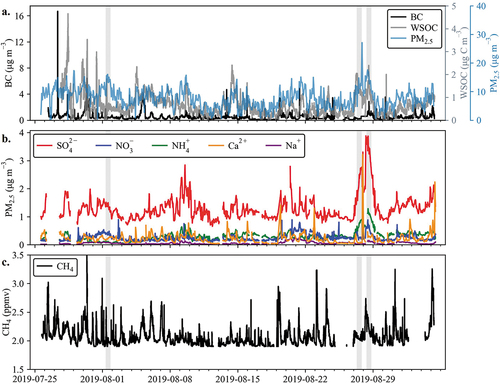
Several BC spikes exceeded 4 µg m⁻³. Although biomass burning can influence CAVE in summer, elevated BC measured in this campaign is likely not from biomass burning given the low concentrations of PM_2.5 levoglucosan (avg. 2.2 ng m⁻³, ranging from 0.17 to 10.1 ng m⁻³), a good tracer for biomass burning (Sullivan et al. 2008), measured throughout the study. NO/NO_x ratios and CH₄ concentrations can be used to investigate possible sources. NO_x is almost entirely emitted from combustion sources as NO; therefore, very fresh (minutes old) plumes present NO to NO_x ratios near 1. None of the BC spikes correspond with NO/NO_x ratios greater than 0.32 (study daytime avg. is 0.2), at 2-min time resolution, indicating that the elevated BC values do not come from very local sources, such as a diesel truck passing or idling near the sample inlet. CH₄ is shown in Figure 2c and had an average mixing ratio of 2.1 ppmv (standard deviation of 0.16). The mean methane mixing ratio is 2.9 ppmv (standard deviation of 0.37) for all BC values above 4 µg m⁻³, suggesting that these high BC values could be associated with O/G flaring and/or diesel engine use. This will be further investigated using HYSPLIT back trajectory analysis later in this work.

Figure 2b shows timelines of the highest concentration species measured by the PILS-IC: SO₄^2- (avg 1.3 µg m⁻³), NH₄⁺, (avg 0.30 µg m⁻³), Ca²⁺ (avg 0.22 µg m⁻³), NO₃⁻ (avg 0.16 µg m⁻³), and Na⁺ (avg 0.057 µg m⁻³). The Ca²⁺ timeline exhibits several short-term, concentration spikes reaching as high as 3.2 µg m⁻³, suggesting emissions of soil dust from local erosion of limestone or gypsum deposits. There are significant gypsum (CaSO₄) and dolomite (CaCO₃) deposits in the Permian Basin (Johnson 1997), located near the CAVE monitoring site. Gypsum is a mineral made of Ca²⁺ and SO₄^2- and could explain some of the excess SO₄^2-, discussed later, and the presence of elevated Ca²⁺ concentrations. A significant proportion of the SO₄^2- in White Sands National Park, another national park in the area, resulted from gypsum and other salts in the area during a study by White et al. (2015). The presence of CaCO₃ is challenging to confirm because carbonate cannot be measured directly by ion chromatography. The role of Ca²⁺ in the aerosol chemistry will be investigated further below.

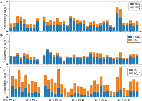
Concentrations of gas-phase NH₃ (avg 0.93 µg m⁻³), HNO₃ (avg 0.89 µg m⁻³), and SO₂ (avg 0.64 µg m⁻³) and PM_2.5 NH₄⁺ (avg 0.47 µg m⁻³), NO₃⁻ (avg 0.27 µg m⁻³), and SO₄²⁺ (avg 1.3 µg m⁻³) measured with the 24-hr URG annular denuder/filter packs are shown in Figure 3. The nitrogen species across nearly all days were dominated by the gas-phase components: NH₃ and HNO₃. Sulfur species were usually dominated by particle phase SO₄^2-. The presence of significant gas-phase HNO₃ and NH₃ illustrates the potential for additional formation of particulate NO₃⁻, either NH₄NO₃ formation under cooler more humid conditions, perhaps at other times of year, or additional coarse particle NO₃⁻ resulting from HNO₃ reactive uptake on sodium chloride or soil dust particles.

Figure 3. URG annular denuder/filter pack sampling shows the particle/gas phase partitioning of (a.) NH₃/NH₄⁺, (b.) HNO₃/ NO₃⁻, and (c.) SO₂/ SO₄^2-. Particle species are shown in Orange, and gas species are shown in blue. There is one day of missing data, 2019–08-04, due to a denuder extraction error.

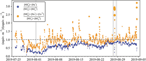
To better understand the aerosol molecular components and look at the pairing of aerosol ions, the concentrations were converted to charge equivalent units. Ions were paired based on likely combinations to form neutral aerosol. Figure 4a indicates that PM_2.5 SO₄^2- is only partially neutralized by NH₄⁺, with an average NH₄⁺ to SO₄^2- charge equivalent ratio of 0.6. Twenty-four-hour NH₃ (g) measured using the URG annular denuders averaged 0.93 µg m⁻³. In such a low humidity environment, it is expected that acidic SO₄^2- aerosol (e.g., sulfuric acid or ammonium bisulfate) would take up NH₃ (g) if available. The coexistence of NH₃ (g) with SO₄^2- not fully neutralized by NH₄⁺ may indicate the presence of a different SO₄^2- particle species.

Figure 4. PILS-IC species (a.) NH₄⁺ and SO₄^2-, and (b.) NO₃⁻ and Na⁺ are shown as nano equivalents m⁻³. Shaded regions represent case study transport dates.

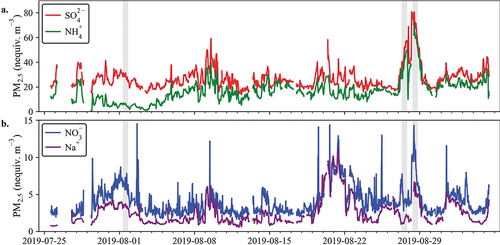
Given that the study was conducted in summertime with high temperatures (avg. 28°C) and low RH (avg. 36%), the formation of significant NH₄NO₃ is not expected. HNO₃ and its precursors can react with other species to form supermicron NO₃⁻ aerosols, such as sodium nitrate (NaNO₃) or calcium nitrate (Ca(NO₃)₂), through reactions with sea salt and soil dust, respectively. Laboratory experiments support the formation of particle NO₃⁻ on sea salt and mineral dust particles from HNO₃ and its precursors (Mamane and Gottlieb 1992). NaNO₃ aerosol will form when sea salt (NaCl) reacts with nitric acid (HNO₃) as shown in Reaction (1) (Pandis and Seinfeld 2016).

(R1) $NaCl\left(s\right)+HN{O}_3\left(g\right)\leftrightarrow NaN{O}_3\left(s\right)+HCl\left(g\right)$(R1)

Comparison of the measured PM_2.5 Cl⁻ to Na⁺ ratios shows that they are consistently below the expected sea salt ratio of 1.16 (Lee et al. 2008), with an average ratio of 0.34 (R² = 0.55), consistent with substantial hydrochloric acid displacement from the aerosol by reaction with nitric acid. A plot of this data can be found in the supplementary materials. Correlated concentration timelines of Na⁺ and NO₃⁻ (Figure 4b; R² = 0.63) suggest that nitric acid displacement of chloride from sea salt may be important in this environment.

Reaction (2) shows HNO₃ reaction with calcium carbonate (CaCO₃) in soil dust which can lead to calcium nitrate aerosol formation.

(R2) $CaC{O}_3\left(s\right)+2HN{O}_3\left(g\right)\leftrightarrow Ca{\left(N{O}_3\right)}_2\left(s\right)+C{O}_2\left(g\right)+H_{2}O\left(g\right)$(R2)

CaCO₃ and HNO₃ readily react with each other at low RH values (Krueger et al. 2003) and this reaction has been found to be important for NO₃⁻ aerosol formation (Fairlie et al. 2010; Jordan et al. 2003). Reactions of nitric acid with sea salt and soil dust can compete and account for the formation of supermicron NO₃⁻ aerosol of differing composition.

During the Big Bend Regional Aerosol and Visibility Observational (BRAVO) in west Texas, researchers found that NO₃⁻ was mostly associated with sea salt particle Na⁺, but that the formation of Ca(NO₃)₂ was also important on several days (Lee, Kreidenweis, and Collett 2004). Malm et al. (2005) found that in Yosemite National Park aerosol nitrate included both submicron NH₄NO₃ and substantial supermicron NaNO₃ resulting from HNO₃ reaction with sea salt transported inland across California’s Central Valley from the Pacific Ocean. Following these two studies, the coarse mode nitrate was characterized at several rural U.S. locations by Lee et al. (2008). Of the five sites characterized, four had contributions from coarse-mode nitrate: Grand Canyon National Park, Great Smoky Mountains National Park, Brigantine National Wildlife Refuge, and San Gorgonio Wilderness Area. Springtime nitrate at the Southern California San Gorgonio mountain measuring site was mostly comprised of NH₄NO₃, while NaNO₃ and Ca(NO₃)₂ together comprised approximately one-third of the total particle nitrate during measurements in the warmer summertime. Coarse mode nitrate formation from soil and sea salt accounted for the majority of particle nitrate in the Grand Canyon and the Great Smokey Mountains (Lee et al. 2008). Similar findings have also been reported outside the United States. Li and Shao (2009) found the formation of Ca(NO₃)₂ to have a significant impact on brown haze episodes in northern China. Global simulations of the effects of mineral dust on aerosol nitrate found that nitrate concentrations in southern Europe, western U.S., and northeastern China are significantly impacted by mineral dust (Karydis et al. 2016). Across the globe, Karydis et al. found that the near surface fine mode nitrate increased by 21% when mineral dust reactions were included.

HNO₃ (g) was present on all days during the 2019 CarCavAQS study period (see Figure 3). While much of the PM_2.5 NO₃⁻ can be explained by a reaction between sea salt and HNO₃, the fact that NO₃⁻ equivalent concentrations exceed Na⁺ equivalent concentrations suggests that an additional form of NO₃⁻ is also present. Reaction (2) is likely, given the elevated Ca²⁺ concentrations, availability of HNO₃, and presence of limestone deposits in the area.

Figure 5 examines the ratio of cations and anions measured by the PILS-IC system more holistically. Ratios of Na⁺ plus NH₄⁺ to SO₄^2- plus NO₃⁻ always fall below unity, indicating an excess of anion species as discussed above. The presence of substantial NH₃ (g) makes it unlikely that the aerosol is acidic enough for H⁺ to balance the excess anion levels. Adding Ca²⁺ to the (cation) numerator changes the story significantly. Currently many of the observations exhibit a cation/anion ratio close to 1, consistent with aerosol charge balance. There does appear to be a period of acidic aerosol from 07/30/2019 to 08/03/2019 and there are several shorter periods where the cation/anion ratio is above 1.0 and even exceeding 2.0. The vales where the ratio is the highest are associated with high Ca²⁺ concentrations. The deficiency in measured anion aerosol species during these periods likely represents the presence of considerable carbonate in this dust-rich aerosol (to be discussed further in section 3.2). As mentioned earlier, carbonate is not detected by ion chromatography. Figure 5 indicates that Ca²⁺ plays an important role in the PM_2.5 aerosol balance, likely as either gypsum or calcium nitrate.

Figure 5. The ratio of cation to anion species measured by the PILS-IC is plotted in equiv. m⁻³. The dotted gray line shows a ratio of unity. The radius of the Orange point size changes proportionally with Ca²⁺ concentration. Shaded regions represent case study transport dates.

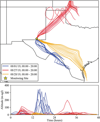
Transport during different aerosol composition periods was considered to help better understand how different source types and regions influence CAVE aerosol composition. HYSPLIT back-trajectories shown in Figure 6, were run for 48 hours. A set of daytime (08:00 to 20:00) trajectories is shown for the period of acidic aerosol on 08/01/19 (see Figure 5), the period of highest gaseous NH₃ on 08/27/19 (see Figure 3), and the largest total PM_2.5 concentration from the PILS-IC on 08/28/19 (see Figure 2a). Only the daytime trajectories are considered here due to increased variability in transport patterns overnight. Transport on 08/27/19 comes from the northeast and passes near two major coal-fired power plants shown in Figure 1, which could be a source of the observed increase in sulfur compounds. This region also includes the largest agricultural production in the area based on the 2017 USDA Census of Agriculture (see map in the supplementary materials), consistent with elevated NH₃ and NH₄⁺ observed in the URG data on this date. Transport on 08/28/19 comes from the southeast over the largest concentration of O/G wells in the region and connects down to the Gulf of Mexico. This 48-hr transport pattern illustrates the importance of the Gulf of Mexico as a sea salt source region to support the reaction with HNO₃ and the formation of NaNO₃ discussed above. Measured aerosol on this date showed evidence of chloride depletion and correlation between PM_2.5 Na⁺ and NO₃⁻. The period of acidic aerosol on 08/01/19 also features transport from the southeast but shifted further south and moving more slowly than the 8/28/19 transport pattern. The air mass sampled at CAVE on this date has more limited NH₃ from the URG denuder measurements and NH₄⁺, consistent with the more acidic aerosol and the lack of major agricultural emissions in the upwind region. The gas-phase species CH₄ and NO_x also have distinct patterns across the 3 days considered, with both low on 08/01 and 08/27 and elevated on 08/28. The CH₄ patterns can be seen clearly in the gray shaded regions of Figure 2c. Conversely, gaseous NH₃ was low on 08/01 and 08/28 and elevated on 08/27. Low CH₄ and NO_x values on 08/01 are consistent with the sampled air masses passing to the south and west of the concentrated O/G region (see Figure 1). High CH₄ and NO_x mixing ratios on 08/28 correspond with a high period of NO₃⁻ and Na⁺, reflecting the importance of transport over the Permian O/G source region and upwind reactions between HNO₃ and sea salt. NO₃⁻ and Na⁺ are consistently elevated from 08/20 through 08/22. The transport patterns for these days are consistent with 08/28 and have dominant transport from the Gulf of Mexico over the Permian O/G region. Overall transport patterns observed in the study will be considered in more detail in section 3.4.

Figure 6. 48-hour HYSPLIT Back Trajectories are shown for three different transport patterns during the study. The bottom panel shows back trajectory altitudes above ground level. The dates were selected based on aerosol composition. For each date 12 daytime back trajectories of 48-hour duration are plotted.

Measurement Comparisons and Mass Closure

PILS-TOC data averaged to daily frequency accounted for on average 78% of the IMPROVE OC. A value less than 100% is expected due to the presence of non-water-soluble OC components. Major species measured directly by IMPROVE and by the PILS (SO₄^2-, NO₃⁻, Ca²⁺, and Na⁺) agreed reasonably well, differing by less than 25% on average. Some difference is expected for calcium due to the differences in measuring water-soluble Ca²⁺ in the PILS-IC vs. elemental Ca in IMPROVE samples. IMPROVE Ca values were generally higher than PILS-IC Ca²⁺ values, consistent with expectations. Measured PM_2.5 mass was compared between the IMPROVE and the TEOM data sets and differed by an average of 13%. A least squares linear regression, forced through the origin, between the paired values had a slope of 0.9 and a strong correlation (R² = 0.79). Comparison figures between the aerosol mass and composition data sets can be found in the supplementary materials.

The sum of mass concentrations of the higher time resolution speciated PM_2.5 measurements (PILS-IC species, BC, and WSOC multiplied by a factor of 1.8 to account for species beyond carbon in the organic aerosol) (Prenni et al. 2019) did not reach full mass closure when compared with the total PM_2.5 mass measured by the TEOM. This is not surprising given the regional importance of insoluble or unquantified components tof airborne dust. The mean difference between the sum of the specified species and the total PM_2.5 mass was 43%.

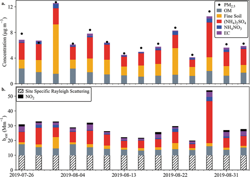
A timeline of the reconstructed PM_2.5 mass from the IMPROVE measurements is plotted in Figure 7a. On average, the IMPROVE reconstructed mass represents 85% of the measured IMPROVE PM_2.5 mass, ranging from 73% to 96%. The analysis of the IMPROVE filters includes elemental species by XRF, which captures the non-water-soluble mineral dust fraction of PM_2.5 aerosol, as well as OC (vs. WSOC in the PILS). The reconstructed mass contains a significant contribution (average of 29.6% and maximum of 64.9%) from fine soil, calculated using Equation 2(2) $FineSoil=2.2\ast \left[Al\right]+2.49\ast \left[\mathrm{S}\mathrm{i}\right]+1.94\ast \left[\mathrm{T}\mathrm{i}\right]+1.63\ast \left[\mathrm{C}\mathrm{a}\right]+2.42\ast \left[\mathrm{F}\mathrm{e}\right]$(2) . This large contribution is consistent with the significant shortfall (average of 43%) in mass closure for the higher time resolution PILS aerosol measurements. IMPROVE mass reconstruction assumes that NO₃⁻ is present as NH₄NO₃ and the SO₄^2- as (NH₄)₂SO₄. Although the PILS-speciated data suggest that the NO₃⁻ is likely present as a mix of NaNO₃ and Ca(NO₃)₂, this does not greatly impact the overall mass closure given the small amounts of NO₃⁻ measured and the similarity of the (charge) equivalent weights of Na⁺, Ca²⁺, and NH₄⁺. The CAVE site-specific Rayleigh scattering is 10 Mm⁻¹.

Figure 7. (a.) IMPROVE mass closure is plotted in the upper panel. Reconstructed PM_2.5 mass is shown as the sum of OM, fine soil, (NH₄)₂SO₄, NH₄NO₃, and EC. The IMPROVE measured PM_2.5 mass is also shown by the black dots. (b.) The contribution to light extinction from each species plotted in (a.) as calculated using the second IMPROVE algorithm for light extinction. Site specific Rayleigh Scattering (10 Mm⁻¹) and NO₂ light extinction are also included. NO₂ (g) light extinction is calculated using the second IMPROVE algorithm and a daily mean of the measured NO_2.

Visibility impacts

Recent work by Hand et al. (2020) looking at 1990–2018 trends across the United States indicates that haze formation in the Intermountain West/Southwest has decreased by ~1% per year, less than in many other regions. From 1990 to 2018, haze contributions by species have shifted to lower sulfate and more influence from carbonaceous aerosol and mineral dust. Average annual haze levels across the Intermountain West/Southwest region had an aerosol light extinction value similar to the background Rayleigh scattering value (10 Mm⁻¹) (Hand et al. 2020). The 2019 measurements in CAVE are the first for this specific park.

Figure 7b shows the 24-hr light extinction values from each of the PM_2.5 species (OM, fine soil, (NH₄)₂SO₄, NH₄NO₃, and EC) measured by the CAVE IMPROVE filters. These values were calculated using the second IMPROVE algorithm (Pitchford et al. 2007; Prenni et al. 2019). This light extinction calculation assumes that NO₃⁻ is present as NH₄NO₃. Light extinction is based on refractive index, assumed size distribution, and hygroscopicity, which differ for NH₄NO₃ vs. NaNO₃ or Ca(NO₃)₂. In the end, however, the 24-hr light extinction from NO₃⁻ is a small contributor relative to other species.

The reconstructed PM_2.5 light extinction for IMPROVE sample days is typically dominated by SO₄^2-, with a mean fractional contribution of 43% and a range from 28% to 66% during the study. Extinction by organic matter, EC, fine soil, and NH₄NO₃ average 27%, 12%, 12%, and 5.3%, respectively. OM was the largest contributor to particle light extinction on 3 days (July 26, August 4, and 25). Fine soil was the largest contributor on August 1, 2019. Although SO₄^2- generally dominates the particle light extinction, the presence of carbonaceous aerosol and mineral dust as the largest contributors on given days, is consistent with the more regional findings of Hand et al. (2020) discussed above.

To better understand the short-term variability in light extinction and associated aerosol species’ contributions, the second IMPROVE algorithm was also applied to our higher time resolution data sets. To do this several assumptions were needed. Some of these assumptions impact the absolute accuracy of the estimated extinction, but the goal is to ascertain relative variability in light extinction and whether short-term concentration excursions lead to species other than SO₄^2-, OM, or fine soil dominating the extinction budget over periods shorter than the 24-hr IMPROVE sample periods. SO₄^2- and NO₃⁻ were again assumed to be present as (NH₄)₂SO₄ and NH₄NO₃, consistent with the IMPROVE light extinction calculations above. Aethalometer BC (880 nm) was assumed to be a good proxy for EC. To estimate fine soil, study average IMPROVE concentrations were used for each elemental species in Equation 2(2) $FineSoil=2.2\ast \left[Al\right]+2.49\ast \left[\mathrm{S}\mathrm{i}\right]+1.94\ast \left[\mathrm{T}\mathrm{i}\right]+1.63\ast \left[\mathrm{C}\mathrm{a}\right]+2.42\ast \left[\mathrm{F}\mathrm{e}\right]$(2) , except for calcium. Calcium exhibited the largest range of fractional contribution to IMPROVE fine soil by a significant margin and was the only species in the IMPROVE soil equation measured in the PILS. The PILS, however, measured water-soluble Ca²⁺ ion, which represents a fraction of the elemental Ca present and measured by XRF in the IMPROVE samples. A comparison of PILS Ca²⁺ vs. IMPROVE Ca revealed that water-soluble Ca²⁺ compromised an average of 78% of elemental Ca, with a range of 48% to 100%, indicating that our substitution of Ca²⁺ for Ca in the IMPROVE soil equation represents a lower bound on that component of fine soil. PILS WSOC was used as a surrogate for OC, so we are again estimating a lower bound for the OC contribution to light extinction. The IMPROVE scale factor (1.8) was used to convert WSOC to OM.

Utilizing these assumptions, averaging high time resolution concentration measurements to 1 hr, and making use of hourly meteorological data from the National Park Service at CAVE, light extinction was calculated at hourly time frequency (Figure 8). The maximum b_ext values, likely lower bounds as discussed above, reach 90 Mm⁻¹ vs. a daily maximum of 54 Mm⁻¹ determined from the IMPROVE measurements.

Figure 8. The second IMPROVE equation was applied to higher time resolution composition data sets (PILS-IC, PILS-TOC, and Aethalometer BC) to estimate hourly light extinction values. These values include the Rayleigh background contribution as well as extinction from NO₂. Fractional light extinction contributions, excluding Rayleigh background, from different species are shown for three data points (shown as blue triangles) as examples. Extinction peaks highlighting maximum contributions are represented by points a and c (30 July 2019 09:00 MST and 28 August 2019 12:00 MST). Point b represents a low light extinction period on 18 August 2019 12:00 MST.

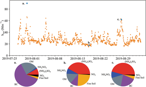
The b_ext peaks represented by points “a” and “c” in Figure 8 highlight maximum contributions to light extinction by different species. Point “a” has a majority contribution from BC. As discussed earlier, the NO/NO_x ratio at this time is low (ratio of 0.22) and similar to other time periods (daytime avg 0.2), likely ruling out a very local combustion source (e.g., an idling vehicle near the inlet), as does the duration of this extinction event across multiple hours. A high CH₄ mixing ratio of 3.16 ppmv (area background of 2 ppmv) coinciding with this light extinction peak suggests O/G activity, likely flaring or diesel engine emissions, as a source of the BC that dominates this 90 Mm⁻¹ hourly extinction episode. Both points “b” and “c”, with low and high hourly b_ext respectively, have the largest extinction contributions from SO₄^2-, similar to the typical pattern at daily time resolution using the IMPROVE data. Both high extinction points (a and c) have corresponding NOAA HYSPLIT back-trajectories that indicate transport from the southeast, a region of intense O/G development and production. The high variability in hourly light extinction values and the different aerosol compositions during peak extinction episodes point to the importance of high time resolution measurements to adequately characterize peaks in visibility impairment in the park and the activities responsible for those episodes.

Residence time analysis

Incremental probability (IP) distributions for the residence time analyses conducted for major species and associated light extinction are presented in Figure 9. Red grid cells indicate that an air mass was more likely to have passed through that grid cell on a high concentration/extinction trajectory (top 10% of parameter values) than during the full set of study back-trajectories. Blue grid cells indicate that passage of a trajectory through that cell was more likely during the full trajectory set than on a high concentration/extinction trajectory.

Figure 9. Incremental probability distributions are plotted for 7 species measured directly during the field campaign: SO₄^2-, NH₄⁺, WSOC, Ca²⁺, NO₃⁻, BC, and CH₄ and 1 calculated value: particle light extinction (b_ext). The IPs are based on 24-hr back trajectories and are distance normalized. This is done by multiplying each grid cell value by the distance from the origin site, shown as a black dot. The grid cell resolution is 0.25 degrees square.

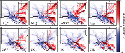
High concentration periods of SO₄^2-, NH₄⁺, and WSOC show prevailing directionality from the SE and from the NE. The high concentration trajectory similarity for SO₄^2- and NH₄⁺ reflects the tight association of aerosol NH₄⁺ with SO₄^2-. As discussed above, coal-fired power plants and agricultural activity to the NE may contribute to increased SO₄^2- and NH₃/NH₄⁺ concentrations during this transport pattern. The light extinction plot (b_ext) shows that the most haze-impacted periods are more strongly associated with transport from the SE, although some influence from the NE remains. The bottom row of species in the figure (Ca²⁺, NO₃⁻, BC, and CH₄) shows the highest concentration measurement periods strongly associated with transport from the SE. The SE sector corresponds with the highest concentration of nearby O/G activity, a likely source of NO₃⁻ precursor NO_x, BC, and CH₄. The SE sector also corresponds with Permian Basin limestone deposits, a likely source of soil dust rich in calcium carbonate. Transport from this direction can also bring sea salt from the Gulf of Mexico, as discussed above, providing an additional path to generate aerosol NO₃⁻ via HNO₃ uptake on sea salt.

Summary

The CarCavAQS study in Carlsbad Caverns National Park provided novel and important insight into the composition and likely sources of particulate matter in the region. PM_2.5 mass ranged up to 31.8 µg m⁻³ with major inorganic contributions from SO₄^2-, NH₄⁺, NO₃⁻, Na⁺, and Ca²⁺. BC and WSOC ranged up to 16.7 µg m⁻³ and 4.7 µg C m⁻³, respectively. Fine particle SO₄^2- is partially neutralized by NH₄⁺, but likely also includes a component from gypsum (CaSO₄) found in regional soils. Summertime NO₃⁻ appears to be present as a result of abundant HNO₃ or its precursors reacting with NaCl from sea salt and CaCO₃ from mineral dust. The gas phases NH₃ and HNO₃ exceed their particle-phase counterparts throughout the study. Forty-eight-hour back trajectory analysis of three distinct transport patterns indicates that air masses often pass through regions with substantial O/G activity when transported to the site from the SE. Transport from this direction often originates over the Gulf of Mexico, carrying sea salt which can react with O/G emissions such as HNO₃ or its precursors. Episodes of high BC concentrations appear to be associated with O/G activity. Aerosol light extinction showed considerable variability at hourly timescales, reaching a maximum of 90 Mm⁻¹ during the study. This temporal variability illustrates the importance of high time resolution measurements for understanding peaks in regional haze at protected locations. While SO₄^2-, on average, was the largest fine particle contributor to light extinction, BC, likely emitted by the abundant flaring or other Permian Basin O/G activities, was found to dominate one of the haziest periods. The highest concentration/light extinction air masses were transported predominantly from the SE, a region with a high density of Permian Basin O/G operations. Future anticipated increases in O/G extraction in the area could exacerbate the air quality problems documented during this study.

Acknowledgment

The authors thank officials at Carlsbad Caverns National Park for providing study access and logistical support. This work was supported by the National Park Service under Agreement Number P20AC00679 with Colorado State University.

Disclosure statement

No potential conflict of interest was reported by the author(s).

Data availability statement

The data that support the findings of this study are available from the corresponding author, Jeffrey L. Collett, upon reasonable request. https://doi.org/10.25675/10217/235481.

Supplementary material

Supplemental data for this article can be accessed online at https://doi.org/10.1080/10962247.2022.2081634

Additional information

Funding

This work was supported by the National Park Service [P20AC00679].

Notes on contributors

Lillian E. Naimie

Lillian E. Naimie received a B.A. in Chemistry from Colby College. She is currently a Ph.D. student at Colorado State University in Atmospheric Science.

Amy P. Sullivan

Amy P. Sullivan is a Research Scientist III in Atmospheric Science at Colorado State University.

K.B. Benedict

K.B. Benedict is a Research Scientist at Los Alamos National Laboratory. During the data collection of this work, she was a Research Scientist in Atmospheric Science at Colorado State University.

Anthony J. Prenni

Anthony J. Prenni is a chemist in the Air Resources Division of the National Park Service.

B.C. Sive

B.C. Sive is an atmospheric chemist in the Air Resources Division of the National Park Service where he serves as the Program Manager for the Gaseous Pollutant Monitoring Program (GPMP).

Bret A. Schichtel

Bret A. Schichtel is a physical scientist in the Air Resource Division of the National Park Service and an affiliate Research Scientist at the CSU-Cooperative Institute for Research in the Atmosphere.

Emily V. Fischer

Emily V. Fischer is an Associate Professor of Atmospheric Science at Colorado State University.

Ilana Pollack

Ilana Pollack is a Research Scientist III in Atmospheric Science at Colorado State University.

Jeffrey Collett

Jeffrey Collett, Jr. is a Professor and Department Head for Atmospheric Science at Colorado State University.

References

- Allegrini, I., F. De Santis, V. Di Palo, A. Febo, C. Perrino, M. Possanzini, and A. Liberti. 1987. Annular denuder method for sampling reactive gases and aerosols in the atmosphere. Sci. Total Environ. 67 (1):1–16. doi:10.1016/0048-9697(87)90062-3.
- Allegrini, I., A. Febo, C. Perrino, and P. Masia. 1994. Measurement of atmospheric nitric acid in gas phase and nitrate in particulate matter by means of annular denuders. Int. J. Environ. Anal. Chem. 54 (3):183–201. doi:10.1080/03067319408034088.
- Allen, D. T., D. Smith, V. M. Torres, and F. C. Saldaña. 2016. Carbon dioxide, methane and black carbon emissions from upstream oil and gas flaring in the United States. Curr. Opin. Chem. Eng. 13:119–23. doi:10.1016/j.coche.2016.08.014.
- Benedict, K. B., C. M. Carrico, S. M. Kreidenweis, B. Schichtel, W. C. Malm, and J. L. Collett. 2013. A seasonal nitrogen deposition budget for Rocky Mountain National Park. Ecol. Appl. 23 (5):1156–69. doi:10.1890/12-1624.1.
- Benedict, K. B., A. J. Prenni, M. M. H. El-Sayed, A. Hecobian, Y. Zhou, K. A. Gebhart, B. C. Sive, B. A. Schichtel, and J. L. Collett. 2020. Volatile organic compounds and ozone at four national parks in the southwestern United States. Atmos. Environ. 239:117783. doi:10.1016/j.atmosenv.2020.117783.
- Bond, T. C., B. Wehner, A. Plewka, A. Wiedensohler, J. Heintzenberg, and R. J. Charlson. 2006. Climate-relevant properties of primary particulate emissions from oil and natural gas combustion. Atmos. Environ. 40 (19):3574–87. doi:10.1016/j.atmosenv.2005.12.030.
- Bond, T. C., S. J. Doherty, D. W. Fahey, P. M. Forster, T. Berntsen, B. J. DeAngelo, M. G. Flanner, S. Ghan, B. Kärcher, D. Koch, et al. 2013. Bounding the role of black carbon in the climate system: A scientific assessment. J. Geophys. Res. Atmos. 118 (11):5380–552. doi:10.1002/jgrd.50171.
- Böttcher, K., -V.-V. Paunu, K. Kupiainen, M. Zhizhin, A. Matveev, M. Savolahti, Z. Klimont, S. Väätäinen, H. Lamberg, and N. Karvosenoja. 2021. Black carbon emissions from flaring in Russia in the period 2012–2017. Atmos. Environ. 254:118390. doi:10.1016/j.atmosenv.2021.118390.
- Brown, D., C. Lewis, and B. Weinberger. 2015. Human exposure to unconventional natural gas development: A public health demonstration of periodic high exposure to chemical mixtures in ambient air. J. Environ. Sci. Health. A Tox. Hazard. Subst. Environ. Eng. 50:460–72. doi:10.1080/10934529.2015.992663.
- Chow, J. C., J. G. Watson, L. W. A. Chen, M. C. O. Chang, N. F. Robinson, D. Trimble, and S. Kohl. 2007. The IMPROVE_A temperature protocol for thermal/optical carbon analysis: Maintaining consistency with a long-term database. J. Air Waste Manage. Assoc. 57 (9):1014–23. doi:10.3155/1047-3289.57.9.1014.
- Clements, N., J. B. Milford, S. L. Miller, W. Navidi, J. L. Peel, and M. P. Hannigan. 2013. Errors in coarse particulate matter mass concentrations and spatiotemporal characteristics when using subtraction estimation methods. J. Air Waste Manage. Assoc. 63 (12):1386–98. doi:10.1080/10962247.2013.816643.
- Conrad, B. M., and M. R. Johnson. 2019. Mass absorption cross-section of flare-generated black carbon: Variability, predictive model, and implications. Carbon 149:760–71. doi:10.1016/j.carbon.2019.04.086.
- Drinovec, L., G. Močnik, P. Zotter, A. S. H. Prévôt, C. Ruckstuhl, E. Coz, M. Rupakheti, J. Sciare, T. Müller, A. Wiedensohler, et al. 2015. The ”dual-spot” Aethalometer: An improved measurement of aerosol black carbon with real-time loading compensation. Atmos. Meas. Tech. 8 (5):1965–79. doi:10.5194/amt-8-1965-2015.
- Eatough, D. J., A. Wadsworth, D. A. Eatough, J. W. Crawford, L. D. Hansen, and E. A. Lewis. 1993. A multiple-system, multi-channel diffusion denuder sampler for the determination of fine-particulate organic material in the atmosphere. Atmospheric Environment. Part A. General Topics 27 (8):1213–19. doi:10.1016/0960-1686(93)90247-V.
- Elvidge, C. D., D. Ziskin, K. E. Baugh, B. T. Tuttle, T. Ghosh, D. W. Pack, E. H. Erwin, and M. Zhizhin. 2009. A fifteen year record of global natural gas flaring derived from satellite data. Energies 2 (3):595–622. doi:10.3390/en20300595.
- Evanoski-Cole, A. R., K. A. Gebhart, B. C. Sive, Y. Zhou, S. L. Capps, D. E. Day, A. J. Prenni, M. I. Schurman, A. P. Sullivan, Y. Li, et al. 2017. Composition and sources of winter haze in the Bakken oil and gas extraction region. Atmos. Environ. 156:77–87. doi:10.1016/j.atmosenv.2017.02.019.
- Fairlie, T. D., D. J. Jacob, J. E. Dibb, B. Alexander, M. A. Avery, A. van Donkelaar, and L. Zhang. 2010. Impact of mineral dust on nitrate, sulfate, and ozone in transpacific Asian pollution plumes. Atmos. Chem. Phys 10 (8):3999–4012. doi:10.5194/acp-10-3999-2010.
- Field, R. A., J. Soltis, M. C. McCarthy, S. Murphy, and D. C. Montague. 2015. Influence of oil and gas field operations on spatial and temporal distributions of atmospheric non-methane hydrocarbons and their effect on ozone formation in winter. Atmos. Chem. Phys 15 (6):3527–42. doi:10.5194/acp-15-3527-2015.
- Fitz, D. R. 2002. Evaluation of Diffusion Denuder Coatings for Removing Acid Gases from Ambient AirRep. University of California, Riverside: Office of Air Quality Planning and Standards, U.S. Environmental Protection Agency.
- Gaswirth, S. B., K. L. French, J. K. Pitman, K. R. Marra, T. J. Mercier, H. M. Leathers-Miller, C. J. Schenk, M. E. Tennyson, C. A. Woodall, and M. E. Brownfield, et al. 2018. Assessment of undiscovered continuous oil and gas resources in the Wolfcamp Shale and Bone Spring Formation of the Delaware Basin, Permian Basin Province, New Mexico and Texas, 2018. Report Rep. 2018-3073, Reston, VA. https://doi.org/10.3133/fs20183073
- Gebhart, K. A., D. E. Day, A. J. Prenni, B. A. Schichtel, J. L. Hand, and A. R. Evanoski-Cole. 2018. Visibility impacts at Class I areas near the Bakken oil and gas development. J. Air Waste Manage. Assoc. 68 (5):477–93. doi:10.1080/10962247.2018.1429334.
- Gebhart, K., R. Farber, J. Hand, D. Eatough, B. Schichtel, J. Vimont, M. Green, and W. Malm. 2021. Long-Term trends in particulate sulfate at grand canyon national park. Atmos. Environ. 253:118339. doi:10.1016/j.atmosenv.2021.118339.
- Hand, J. L., A. J. Prenni, S. Copeland, B. A. Schichtel, and W. C. Malm. 2020. Thirty years of the Clean Air Act Amendments: Impacts on haze in remote regions of the United States (1990–2018. Atmos. Environ. 243:117865. doi:10.1016/j.atmosenv.2020.117865.
- Hansen, A. D. A., H. Rosen, and T. Novakov. 1984. The aethalometer — An instrument for the real-time measurement of optical absorption by aerosol particles. Sci. Total Environ. 36 (36):191–96. doi:10.1016/0048-9697(84)90265-1.
- Hecobian, A., A. L. Clements, K. B. Shonkwiler, Y. Zhou, L. P. MacDonald, N. Hilliard, B. L. Wells, B. Bibeau, J. M. Ham, J. R. Pierce, et al. 2019. Air toxics and other volatile organic compound emissions from unconventional oil and gas development. Environ. Sci. Technol. Lett. 6 (12):720–26. doi:10.1021/acs.estlett.9b00591.
- Homeland Infastructure Foundation-Level Data (HIFLD). 2019. Oil and natural gas wells. Accessed February 26, 2021. https://gii.dhs.gov/HIFLD.
- Johnson, K. S. 1997. Permian evaporites in the Permian Basin of southwestern United States. Pr. Państw. Inst. Geol. (157 PART 2):95–96.
- Jordan, C., J. Dibb, B. Anderson, M. H. Hecht, S. M. Grannan-Feldman, K. Manatt, S. J. West, X. Wen, M. Frant, and T. Gillette. 2003. Uptake of nitrate and sulfate on dust aerosols during TRACE-P. J. Geophys. Res 108:13-1 - 13–12. doi:10.1029/2002JD003101.
- Karydis, V. A., A. P. Tsimpidi, A. Pozzer, M. Astitha, and J. Lelieveld. 2016. Effects of mineral dust on global atmospheric nitrate concentrations. Atmos. Chem. Phys 16:1491–509. doi:10.5194/acp-16-1491-2016.
- Khalek, I. A., M. G. Blanks, P. M. Merritt, and B. Zielinska. 2015. Regulated and unregulated emissions from modern 2010 emissions-compliant heavy-duty on-highway diesel engines. J. Air Waste Manage. Assoc. 65 (8):987–1001. doi:10.1080/10962247.2015.1051606.
- Krueger, B. J., V. H. Grassian, A. Laskin, and J. P. Cowin. 2003. The transformation of solid atmospheric particles into liquid droplets through heterogeneous chemistry: Laboratory insights into the processing of calcium containing mineral dust aerosol in the troposphere. Geophys. Res. Lett. 30 (3). doi: 10.1029/2002GL016563.
- Lee, T., S. M. Kreidenweis, and J. L. Collett. 2004. Aerosol ion characteristics during the big bend regional aerosol and visibility observational study. J. Air Waste Manage. Assoc. 54 (5):585–92. doi:10.1080/10473289.2004.10470927.
- Lee, T., X.-Y. Yu, B. Ayres, S. M. Kreidenweis, W. C. Malm, and J. L. Collettjr. 2008. Observations of fine and coarse particle nitrate at several rural locations in the United States. Atmos. Environ. 42 (11):2720–32. doi:10.1016/j.atmosenv.2007.05.016.
- Li, W. J., and L. Y. Shao. 2009. Observation of nitrate coatings on atmospheric mineral dust particles. Atmos. Chem. Phys 9:1863–71. doi:10.5194/acp-9-1863-2009.
- Li, Y., B. A. Schichtel, J. T. Walker, D. B. Schwede, X. Chen, C. M. Lehmann, M. A. Puchalski, D. A. Gay, and J. L. Collett. 2012. Increasing importance of deposition of reduced nitrogen in the United States. Proc. Natl. Acad. Sci. 113:5874– 79. doi:10.1073/pnas.1525736113
- Malm, W. C., B. A. Schichtel, M. L. Pitchford, L. L. Ashbaugh, and R. A. Eldred. 2004. Spatial and monthly trends in speciated fine particle concentration in the United States. J. Geophys. Res. Atmos. 109 (D3). doi: 10.1029/2003JD003739.
- Malm, W. C., D. E. Day, C. Carrico, S. M. Kreidenweis, J. L. Collett, G. McMeeking, T. Lee, J. Carrillo, and B. Schichtel. 2005. Intercomparison and closure calculations using measurements of aerosol species and optical properties during the Yosemite Aerosol Characterization Study. J. Geophys. Res 110:D14302. doi:10.1029/2004JD005494.
- Malm, W. C. 2016. Chapter 1 - Introduction. In Visibility, 1–27. Elsevier. doi:10.1016/B978-0-12-804450-6.00001-2.
- Mamane, Y., and J. Gottlieb. 1992. Nitrate formation on sea-salt and mineral particles—a single particle approach. Atmos. Environ. A, Gen. Top. 26 (9):1763–69. doi:10.1016/0960-1686(92)90073-T.
- Olaguer, E. P. 2012. The potential near-source ozone impacts of upstream oil and gas industry emissions. J. Air Waste Manage. Assoc. 62 (8):966–77. doi:10.1080/10962247.2012.688923.
- Orsini, D., Y. Ma, A. Sullivan, B. Sierau, K. Baumann, and R. Weber. 2003. Refinements to the particle-into-liquid sampler (PILS) for ground and airborne measurements of water-soluble aerosol composition. Atmos. Environ. 37:1243–59. doi:10.1016/S1352-2310(02)01015-4.
- Pandis, S. N., and J. H. Seinfeld. 2016. Atmospheric chemistry and physics: From air pollution to climate change. Hoboken, NJ: Wiley-Blackwell.
- Petzold, A., J. A. Ogren, M. Fiebig, P. Laj, S. M. Li, U. Baltensperger, T. Holzer-Popp, S. Kinne, G. Pappalardo, N. Sugimoto, et al. 2013. Recommendations for the interpretation of “black carbon” measurements. Atmospheric Chem. Phys. 13. doi:10.5194/acpd-13-9485-2013.
- Pitchford, M., W. Malm, B. Schichtel, N. Kumar, D. Lowenthal, and J. Hand. 2007. Revised Algorithm for Estimating Light Extinction from IMPROVE Particle Speciation Data. J. Air Waste Manage. Assoc. 57 (11):1326–36. doi:10.3155/1047-3289.57.11.1326.
- Pollack, I. B., B. M. Lerner, and T. B. Ryerson. 2010. Evaluation of ultraviolet light-emitting diodes for detection of atmospheric NO2 by photolysis - chemiluminescence. J. Atmos. Chem. 65 (2):111–25. doi:10.1007/s10874-011-9184-3.
- Prenni, A. J., D. E. Day, A. R. Evanoski-Cole, B. C. Sive, A. Hecobian, Y. Zhou, K. A. Gebhart, J. L. Hand, A. P. Sullivan, Y. Li, et al. 2016. Oil and gas impacts on air quality in federal lands in the Bakken region: An overview of the Bakken Air Quality Study and first results. Atmos. Chem. Phys 16 (3):1401–16. doi:10.5194/acp-16-1401-2016.
- Prenni, A., J. Hand, W. Malm, S. Copeland, G. Luo, F. Yu, N. Taylor, L. Russell, and B. Schichtel. 2019. An examination of the algorithm for estimating light extinction from IMPROVE particle speciation data. Atmos. Environ. 214:116880. doi:10.1016/j.atmosenv.2019.116880.
- Shen, X., T. Lv, X. Zhang, X. Cao, X. Li, B. Wu, X. Yao, Y. Shi, Q. Zhou, X. Chen, et al. 2021. Real-world emission characteristics of black carbon emitted by on-road China IV and China V diesel trucks. Sci. Total Environ. 799:149435. doi:10.1016/j.scitotenv.2021.149435.
- Stein, A. F., R. R. Draxler, G. D. Rolph, B. J. B. Stunder, M. D. Cohen, and F. Ngan. 2015. NOAA’s HYSPLIT Atmospheric Transport and Dispersion Modeling System. Bull. Am. Meteorol. Soc. 96 (12):2059–77. doi:10.1175/BAMS-D-14-00110.1.
- Sullivan, A., R. Weber, A. Clements, J. Turner, M. Bae, and J. Schauer. 2004. A method for on-line measurement of water-soluble organic carbon in ambient aerosol particles: Results from an urban site. Geophys. Res. Lett. 311. doi:10.1029/2004GL019681.
- Sullivan, A. P., R. E. Peltier, C. A. Brock, J. A. de Gouw, J. S. Holloway, C. Warneke, A. G. Wollny, and R. J. Weber. 2006. Airborne measurements of carbonaceous aerosol soluble in water over northeastern United States: Method development and an investigation into water-soluble organic carbon sources. J. Geophys. Res. Atmos. 111 (D23). doi: 10.1029/2006JD007072.
- Sullivan, A. P., A. S. Holden, L. A. Patterson, G. R. McMeeking, S. M. Kreidenweis, W. C. Malm, W. M. Hao, C. E. Wold, and J. L. Collett Jr. 2008. A method for smoke marker measurements and its potential application for determining the contribution of biomass burning from wildfires and prescribed fires to ambient PM2.5 Organic Carbon. J. Geophys. Res 113:D22302. doi:10.1029/2008JD010216.
- Sullivan, A. P., N. Frank, G. Onstad, C. D. Simpson, and J. L. Collett Jr. 2011a. Application of High-Performance Anion-Exchange Chromatography – Pulsed Amperometric Detection for Measuring Carbohydrates in Routine Daily Filter Samples Collected by a National Network: 1. Determination of the Impact of Biomass Burning in the Upper Midwest. J. Geophys. Res 116:D08302. doi:10.1029/2010JD014166.
- Sullivan, A. P., N. Frank, D. M. Kenski, and J. L. Collett Jr. 2011b. Application of high-Performance Anion-Exchange Chromatography – Pulsed amperometric detection for measuring carbohydrates in routine daily filter samples collected by a national network: 2. examination of sugar alcohols/polyols, sugars, and anhydrosugars in the Upper Midwest. J. Geophys. Res 116:D08303. doi:10.1029/2010JD014169.
- Sullivan, A. P., A. A. May, T. Lee, G. R. McMeeking, S. M. Kreidenweis, S. K. Akagi, R. J. Yokelson, S. P. Urbanski, and J. L. Collett Jr. 2014. Airborne-Based source smoke marker ratios from prescribed burning. Atmos. Chem. Phys 14:10535–45. doi:10.5194/acp-14-10535-2014.
- Sullivan, A. P., H. Guo, J. C. Schroder, P. Campuzano-Jost, J. L. Jimenez, T. Campos, V. Shah, L. Jaeglé, B. H. Lee, F. D. Lopez‐hilfiker, et al. 2019. Biomass burning markers and residential burning in the WINTER aircraft campaign. Journal of Geophysical Research: Atmospheres 124:1846–61. doi:10.1029/2017JD028153.
- Thompson, C. R., J. Hueber, and D. Helmig. 2014. Influence of oil and gas emissions on ambient atmospheric non-methane hydrocarbons in residential areas of Northeastern Colorado. Elementa 3. doi:10.12952/journal.elementa.000035.
- United States Energy Information Administration (EIA). 2021a. Where our natural gas comes from. Accessed November 11, 2021. https://www.eia.gov/energyexplained/natural-gas/where-our-natural-gas-comes-from.php.
- United States Energy Information Administration (EIA). 2021b. Annual Energy Outlook. Accessed November 10, 2021, from https://www.eia.gov/outlooks/aeo/.
- United States Energy Information Administration (EIA). 2022. U.S. Energy mapping system. Accessed March 21, 2022. https://www.eia.gov/state/maps.php.
- United States Environmental Protection Agency (EPA). 1999. Regional haze regulations: Final rule. 40 CFR Part 51. Fed. Regist. 64: 35714–74.
- United States Environmental Protection Agency (EPA). 2019. 2017 national emissions inventory (NEI) data. Environmental Protection Agency. Accessed April 8, 2022, from https://www.epa.gov/air-emissions-inventories/2017-national-emissionsinventory-nei-data
- USDA National Agricultural Statistics Service. 2017. Census of agriculture. www.nass.usda.gov/AgCensus.
- Weber, R. J., D. Orsini, Y. Daun, Y. N. Lee, P. J. Klotz, and F. Brechtel. 2001. A Particle-into-Liquid Collector for Rapid Measurement of Aerosol Bulk Chemical Composition. Aerosol Sci. Technol. 35 (3):718–27. doi:10.1080/02786820152546761.
- Weyant, C. L., P. B. Shepson, R. Subramanian, M. O. L. Cambaliza, A. Heimburger, D. McCabe, E. Baum, B. H. Stirm, and T. C. Bond. 2016. Black carbon emissions from associated natural gas flaring. Environ. Sci. Technol. 50 (4):2075–81. doi:10.1021/acs.est.5b04712.
- White, W. H., N. P. Hyslop, K. Trzepla, S. Yatkin, R. S. Rarig Jr, T. E. Gill, and L. Jin. 2015. Regional transport of a chemically distinctive dust: Gypsum from White Sands, New Mexico (USA. Aeolian Res. 16:1–10. doi:10.1016/j.aeolia.2014.10.001.
- Yanowitz, J., R. L. McCormick, and M. S. Graboski. 2000. In-use emissions from heavy-duty diesel vehicles. Environ. Sci. Technol. 34 (5):729–40. doi:10.1021/es990903w.
- Yu, X.-Y., T. Lee, B. Ayres, S. M. Kreidenweis, J. L. Collett, and W. Malm. 2005. Particulate nitrate measurement using nylon filters. J. Air Waste Manage. Assoc. 55 (8):1100–10. doi:10.1080/10473289.2005.10464721.