Performance evaluation of a recurrent deep neural network optimized by swarm intelligent techniques to model particulate matter

ABSTRACT

Atmospheric pollution refers to the presence of substances in the air such as particulate matter (PM) which has a negative impact in population ́s health exposed to it. This makes it a topic of current interest. Since the Metropolitan Zone of the Valley of Mexico’s geographic characteristics do not allow proper ventilation and due to its population’s density a significant quantity of poor air quality events are registered. This paper proposes a methodology to improve the forecasting of PM10 and PM2.5, in largely populated areas, using a recurrent long-term/short-term memory (LSTM) network optimized by the Ant Colony Optimization (ACO) algorithm. The experimental results show an improved performance in reducing the error by around 13.00% in RMSE and 14.82% in MAE using as reference the averaged results obtained by the LSTM deep neural network. Overall, the current study proposes a methodology to be studied in the future to improve different forecasting techniques in real-life applications where there is no need to respond in real time.

Implications: This contribution presents a methodology to deal with the highly non-linear modeling of airborne particulate matter (both PM10 and PM2.5). Most linear approaches to this modeling problem are often not accurate enough when dealing with this type of data. In addition, most machine learning methods require extensive training or have problems when dealing with noise embedded in the time-series data. The proposed methodology deals with this data in three stages: preprocessing, modeling, and optimization. In the preprocessing stage, data is acquired and imputed any missing data. This ensures that the modeling process is robust even when there are errors in the acquired data and is invalid, or the data is missing. In the modeling stage, a recurrent deep neural network called LSTM (Long-Short Term Memory) is used, which shows that regardless of the monitoring station and the geographical characteristics of the site, the resulting model shows accurate and robust results. Furthermore, the optimization stage deals with enhancing the capability of the data modeling by using swarm intelligence algorithms (Ant Colony Optimization, in this case). The results presented in this study were compared with other works that presented traditional algorithms, such as multi-layer perceptron, traditional deep neural networks, and common spatiotemporal models, which show the feasibility of the methodology presented in this contribution. Lastly, the advantages of using this methodology are highlighted.

Introduction

Airborne pollution

Atmospheric pollution can affect the health of the population exposed to it even in low concentrations of these pollutants (Christidis et al. 2019). The global mortality related to air pollution was found to be 1 million premature deaths in rural and urban areas in 2000, and it was increased to 3.1 million in 2012 and increased to 4.2 million in 2016 (Nikoonahad et al. 2017; WHO 2018). In the Metropolitan Zone of the Valley of Mexico (ZMVM for its acronym in Spanish), airborne pollution, especially particulate matter, has been a growing concern in the fields of health and environment due to its evident trend to growing motorization and industrialization in the area (Pérez-Cirera et al. 2016). These particulate materials include all suspended particles, whether its origin is natural or artificial. According to Yan et al., PM₁₀ (particulate matter having an effective aerodynamic diameter smaller than 10 µm) is introduced as one of the main pollutants (among PM_2.5, NO₂, and O₃) in cities with similar characteristics as the ones in ZMVM (Yan et al. 2019). For example, in Pecan (China), which is a largely populated area similar to ZMVM in terms of industries, transportation, and population, PM₁₀ is responsible for approximately 80% of annual air pollution (Mu et al. 2014). PM₁₀ is highly correlated to hospital admissions due to various health outcomes such as respiratory diseases and cardiovascular diseases (Bodor et al., 2021; Lee, Kim, and Lee 2014). The World Health Organization (WHO) has stated, “There is a strong evidence to conclude that fine particles (PM_2.5, particulate matter having an effective aerodynamic diameter smaller than 2.5 µm) are more hazardous than coarse particles (PM₁₀) in terms of mortality and cardiovascular and respiratory endpoints in panel studies” (WHO 2021).

Recurrent neural networks

For the reasons and possible consequences mentioned above it is highly important to build an accurate and precise model of this pollution for its analysis, to forecast events and trends to take due precautions. Airborne pollution can be classified as a time-dependent practical problem that can be analyzed and predicted as a time series (Hua et al. 2019). These time-series problems are more complex than other statistical data due to the long-term trends, cyclical variations, and seasonal variations. Predicting such highly fluctuating and irregular data is usually subject to large errors (Kumar et al. 2017; Prokuryakov 2017). Learning these long-range dependencies that are embedded in time series is often an obstacle for most algorithms. Recurrent Neural Networks (RNNs) are a powerful model for processing time-series data such as airborne pollution (Chen, Zhou, and Dai 2015). The RNNs refer to neural networks that take as an input their previous state; this means that the neural network will have two inputs, the new information entered in the network and its previous state, as shown in Figure 1.

Figure 1. RNN structure. Adapted from (Yixiang and Chunning 2020).

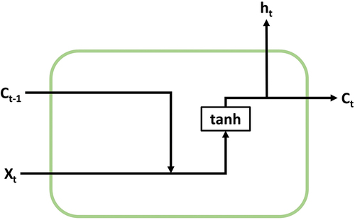
Where X refers to the input of the model, t refers to the time unit being evaluated, C refers to the current state in the unit, and h refers to the output of the model. In 1997, Hochreiter and Schmidhuber proposed the Long Short-Term Memory (LSTM) model, one of the most successful RNN’s architectures (Hochreiter and Schmidhuber 1997). Unlike a simple recurrent neural network, the LSTM model introduces a block of internal memory, composed of simple blocks connected in a specific way (Hua et al. 2019). This internal memory block allows the model to have long-term memory in the form of weights, which is modified during the training of the network and short-term memory defined in activation functions between the communication of the nodes of neurons. The LSTM neuron structure is shown in Figure 2.

Figure 2. Components of LSTM. Adapted from (Yixiang and Chunning 2020).

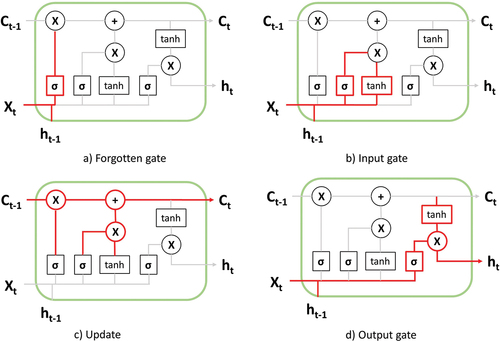
where X refers to the input of the model, t refers to the time unit being evaluated, C refers to the current state in the unit, σ refers to a sigmoid function used by the LSTM unit, and h refers to the output of the model. In addition, for example, h_t refers to the current input being evaluated and h_t−1 to the previous input being evaluated. (a) Forgotten gate: This gate is used to control the state of the cell where the previous state and the input of the LSTM unit pass through a sigmoid function producing a value between 0 (do not allow any data to pass through) and 1 (allow every data to pass through). (b) Input gate: This gate determines the added information to the state cell. It contains two parts: a sigmoid input (input signal control) and a tanh function (the input content). (c) Update: Updates the cell status. (d) Output gate: This gate determines the output of the unit. It contains two parts: a sigmoid function (output signal control) and a tanh function (the output content).

Swarm intelligence

As computer-related technologies are more and more widely used, many NP-hard problems have emerged in areas like big data, spam detection, image processing, and environmental concerns (Faris et al. 2019; Gu et al. 2017; Liu et al. 2019; Zhu et al. 2018). However, when traditional gradient descent and other deterministic methods are used to solve these complicated issues, the degree of finding the global optima, or an acceptable approach, is extremely unsatisfactory in these scenarios (Zhao et al. 2020). Recently, Swarm Intelligence (SI), or Bio-inspired computation, has gained a lot of attention approaching this kind of problems (Nguyen, Xue, and Zhang 2020). The term swarm intelligence was first introduced in 1989 by Gerardo Beni and Jing Wang in order to describe the dynamics of cellular robots that could be framed as a form of intelligent collective behavior, meaning to demonstrate a social intelligence but not a particular intelligence as an individual (Beni and Wang 1993). This marks the point at which swarm behaviors were started to be studied outside natural sciences, although animal behavior has always continued to be a major source of inspiration for swarm intelligence development (Schranz et al. 2021). There are various reasons responsible for the growing popularity of such swarm intelligence-based algorithms, most importantly being the flexibility and versatility offered by these algorithms (Chakraborty and Kar 2017).

Among the concept of swarm intelligence, there is the ant colony optimization algorithm or ACO algorithm (Uthayakumar et al. 2020). The ACO algorithm was proposed by Dorigo in 1992, which has shown excellent performance on several combinatorial problems from different areas (Dorigo, Maniezzo, and Coloni 1996; Wang et al. 2016; Xu, Liu, and Chen 2017). The ACO algorithm is a well-explored metaheuristic evolutionary algorithm based on population, which is inspired by the research results of the collective behavior of real ants in nature. The ACO algorithm relies on the activities of many individualities and feedback of information. Although the activity of an ant is very simple, the activity of a whole ant colony is acceptable (Deng, Xu, and Zhao 2019). ACO has been inspired by the behavior of real ants that enables them to find the shortest paths between food sources and their nest. In the process of finding the shortest path, the ants are guided by exploiting pheromone, which is deposited on the searching space by other ants (Ning et al. 2018).

To solve a combinatorial problem applying the ACO algorithm, the artificial ants choose different positions or nodes in the search space to build a solution. Each of the artificial ants chooses its next move (to the next position) according to the pheromone concentration value. After all the artificial ants complete their solutions, pheromone values are updated after each solution is built (Ismkhan 2017). This process is repeated until the stop condition is met. A simple version of the ACO algorithm is presented in Figure 3 as a flowchart.

Figure 3. Ant colony optimization algorithm.

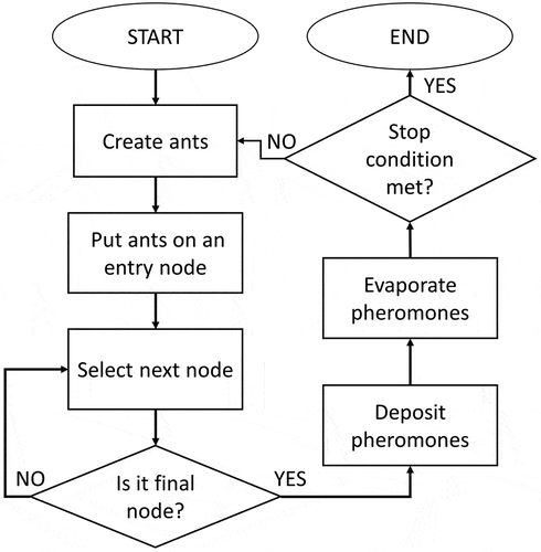
In Figure 3 it can be seen how a simple version of the ACO algorithm works, where ants are created and introduced into an entry state in a search space composed of multiple nodes. Once an artificial ant has built a solution (passing through all nodes), pheromones in the solution are deposited. This pheromone concentration deposited is directly related to how efficient the solution is. At the end of each iteration pheromones in the search space will evaporate at some rate. The evaporation takes place to allow less efficient solutions to get lost through iterations. Finally, if convergence is reached, a stop condition is met where a solution can be identified because it possesses the highest pheromone concentration deposited by the artificial ants (Ghosh et al. 2019; Li, Soleimani, and Zohal 2019).

There are multiple studies that approach forecasting of PM₁₀ and PM_2.5 in Mexico City, through SVM/Kernel functions, ANFIS-BFOA, ANFIS-PSO, GRU, and CNN, due to the high relevance of these pollutants in the area (Aceves et al. 2020; Becerra et al. 2020; Cabrera et al. 2019; Ordeñez et al. 2019; Sotomayor et al. 2013). The objective of this work is to propose a methodology through which the models forecasted for these particles could be improved through ACO using models as the search space for the algorithm.

Material and methods

Materials

The measurement of air pollutants is a complex technical activity that involves the use of specialized equipment, qualified personnel for its operation, and an adequate support and communication infrastructure. In addition to measurement, it is necessary to ensure that the data generated appropriately describe the state of air quality; therefore, the operation of the monitoring program also requires methodologies and standards for measurement, as well as a continuous program of quality assurance.

In operational terms, one of the subsystems that composes the Atmospheric Monitoring System in Mexico City is called Automatic Atmospheric Monitoring Network (or RAMA for its acronym in Spanish). The RAMA uses continuous equipment for the measurement of sulfur dioxide, carbon monoxide, nitrogen dioxide, ozone, PM₁₀, and PM_2.5. It is made up of 34 monitoring stations and has a laboratory for the maintenance and calibration of the monitoring equipment (Government MC 2021).

The stations used in this work were chosen to take into account two considerations:

• The availability of PM10 and PM2.5 data from 2012 to 2019.

• The available data has a maximum of 30% missing data during the whole evaluated period. Otherwise, the forecasting and prediction may be biased.

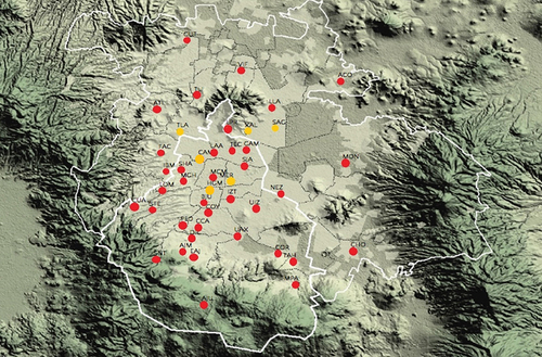
Based in these considerations, six stations were chosen. These stations are San Agustín (SAG), Tlanepantla (TLA), Merced (MER), Xalostoc (XAL), Camarones (CAM), and Hospital General de México (HGM). These stations chosen differ in traffic flow density by a wide range calculated by Tellez using the quantity of vehicles registered per 1000 inhabitants (Tellez, López, and Fernández 2018). These categories of traffic flow density are as follows: low density (XAL, TLA, and SAG), medium density (CAM and MER), and high density (HGM). The locations of these stations are shown in Figure 4 as yellow circles.

Figure 4. All stations available in RAMA (red) and stations used in this work (yellow) (RAMA 2021).

To characterize these stations, three categories were determined based on the zone they are located, and these three categories are:

• Industrial: In an industrial zone, it is expected to have the highest pollutant daily concentrations during working hours. The considered station categorized as industrial in this work will be TLA.

• Commercial: In a commercial zone, it is expected for the pollution to be at its highest peak during meal times, mostly for lunch and dinner. The considered stations categorized as commercial in this work are MER, HGM, and CAM.

• Residential: In a residential zone, it is expected for the pollution to be at its highest peak during the beginning and end of working hours. The considered stations categorized as residential in this work will be SAG and XAL.

Databases available in RAMA display the concentrations of PM₁₀ and PM_2.5 obtained in µg/m3 which are monitored every hour. The total hours considered for these databases were 70,080. However, for different reasons, maintenance, or technical issues, neither of them have the 100% of the data available. Initial missing data, standard deviation calculated through Equation (1)(1) $Std.Dev.=\sqrt{\frac{\sum _{i=1}^n{\left(xi-\bar{x}\right)}^2}{n-1}}$(1) , mean, and quartiles are shown in Table 1.

(1) $Std.Dev.=\sqrt{\frac{\sum _{i=1}^n{\left(xi-\bar{x}\right)}^2}{n-1}}$(1)

Table 1. Initial missing data per particle and station.

Station	Initial missing data		Standard deviation		Mean		Q1		Q2		Q3
	PM2.5	PM10	PM2.5	PM10	PM2.5	PM10	PM2.5	PM10	PM2.5	PM10	PM2.5	PM10
SAG	26.35%	26.35%	15.59	29.14	24.02	50.58	13	30	21	45	32	65
TLA	19.27%	19.24%	15.48	28.07	25.83	52.94	15	33	23	48	34	68
MER	13.64%	13.29%	16.19	27.77	25.97	52.53	14	32	23	48	35	68
XAL	18.28%	18.21%	19.55	37.82	30.03	66.71	16	39	26	58	40	86
HGM	16.49%	16.49%	16.54	24.44	25.29	44.04	14	26	22	40	33	57
CAM	24.02%	24.02%	15.38	25.5	26.3	49.3	15	31	24	45	34	63

Table 2. Evaporation rates and ant quantities tested.

No.	ρ= 0.1%			ρ= 1%			ρ= 5%			ρ= 10%			ρ= 20%
	t(s)	rmse	std.	t(s)	rmse	std.	t(s)	rmse	std	t(s)	rmse	std.	t(s)	rmse	std.
1	2.68	5.53	0.06	2.46	5.51	0.04	2.02	5.48	0.04	1.27	5.49	0.03	1.05	5.5	0.04
3	5.1	5.51	0.03	4.29	5.49	0.04	3.31	5.47	0.05	2.28	5.49	0.05	2.28	5.48	0.05
5	7.48	5.49	0.05	5.24	5.48	0.05	5.5	5.48	0.03	3.41	5.46	0.03	2.97	5.48	0.04
10	9.54	5.49	0.04	8.79	5.48	0.02	6.64	5.46	0.03	6.96	5.47	0.05	5.17	5.47	0.05
25	23.12	5.49	0.03	19.73	5.46	0.04	17.52	5.47	0.03	14.06	5.47	0.05	17.12	5.48	0.05
50	35.6	5.49	0.03	30.42	5.46	0.05	26.73	5.48	0.05	24.41	5.46	0.04	21.8	5.48	0.06

where x_i refers to the ith element of the database, x refers to the mean concentration for the whole data set and n refers to the number of the data points in the data set.

Since it is not convenient to maintain these missing data percentages to continue with the methodology described below, an imputation algorithm needs to be implemented. These missing data are considered random due to its nature mentioned by the National Institute of Ecology (or INE by its acronym in Spanish) which is explained as malfunctions of the equipment (de Ecología IN 2019). The periods in which these data are missing are mostly a few hours, but it may be extended to days in some cases.

Methodology

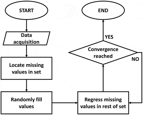
To solve the missing data problem, the Multivariate Imputation by Chained Equations or MICE algorithm was applied to the database with the shape of x ₁, x ₂, …, x_n, where n refers to the length of the dataset and a subset of missing values is present. To implement the MICE algorithm, the first step is to fill the missing data with random values. The first missing value of the set, for instance, x₁, is then regressed on the other variables x₂, …, x_n. The next missing value, x₂, is regressed on all the other variables x₁, x₃, … , x_n. The process is repeated for all other missing values, which in turn is called a cycle (Royston and White 2011). Most authors report that a total of 5 cycles are enough to reach convergence (Beesley and Taylor 2019; Resche-Rigon and White 2016; Wulff and Jeppesen 2017). The full methodology for the MICE algorithm is shown in Figure 5.

Figure 5. Multiple imputation by chained equations (MICE).

To evaluate the MICE algorithm, the MER station was chosen because it is the station with the lowest missing data. This experimentation consisted in creating randomized artificial gaps in the database. The randomized artificial gaps for PM₁₀ and PM_2.5 MER were created to reach a 20% of the total missing data per station, adding 6.71% and 6.36% of randomized artificial gaps, respectively. Distribution between imputed data for real missing data and artificial missing data is shown using histograms in Figures 6 and 7.

Figure 6. Comparison between imputation with real missing PM₁₀ data and randomized missing PM₁₀ data for MER.

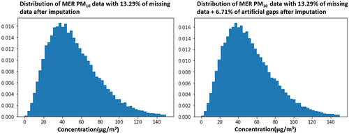
Figure 7. Comparison between imputation with real missing PM_2.5 data and randomized missing PM_2.5 data for MER.

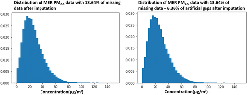
In Figures 6 and 7 are shown how MICE algorithm imputes data for two different cases, where the histograms on the left for both figures describe imputed data for real missing data in database and histograms on the right show an artificial scenario that does not visually differentiate from the real one. To evaluate the MICE algorithm, the standard deviation, Equation (1)(1) $Std.Dev.=\sqrt{\frac{\sum _{i=1}^n{\left(xi-\bar{x}\right)}^2}{n-1}}$(1) , was used for both cases per particle and was calculated resulting in a difference of 0.06 for PM₁₀ and 0.04 for PM_2.5. Furthermore, the mean difference between each corresponding value for the two imputations was calculated resulting in a mean difference of 0.08 for PM₁₀ and −0.22 for PM_2.5. In other words, the MICE algorithm seems to have a successful performance due to this experiment’s minor differences when adding randomized artificial gaps.

Once the imputation stage is complete, the database is full with raw data and well-estimated interpolations. Subsequently, a normalization stage needs to scale all the database between −1 and 1, this scaling is executed through Equation (2)(2) $\frac{value-min}{max-min}$(2) . The (1,1) range was chosen due to the SELU activation function used by (Ramírez-Montañez et al. 2019) that has different behaviors when inputted positive and negative values. The SELU function was introduced and analytically proved by (Klambauer, Unterthiner, and Mayr 2017) which is described in Equation (3)(3) $SELU\left(x\right)=\lambda \left\{\begin{array}{c}xx>0\\ \alpha e^x-\alpha else\end{array}\right.$(3) .

(2) $\frac{value-min}{max-min}$(2)

where value refers to the value being normalized. Also, min and max refer to the minimum and maximum values through all the database. Once the data is normalized between −1 and 1 more efficiency is achieved when training the LSTM model due to its decrease in non-linearity (Chen, Zhou, and Dai 2015).

(3) $SELU\left(x\right)=\lambda \left\{\begin{array}{c}xx>0\\ \alpha e^x-\alpha else\end{array}\right.$(3)

Where λ = 1.0507 and α = 1.6733.

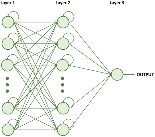
The architecture of the LSTM network is based in (Ramírez-Montañez et al. 2019). This network consists in three layers:

• Layer 1 consists of 50 LSTM neurons, which will take the first 50 data and expand them to feed the second layer, storing them.

• Layer 2 is the hidden layer that consists in 256 LSTM neurons.

• Layer 3 is a simple neuron, which based on the previous recorded data will generate a new value, successively.

The complete model of the LSTM predictive network is shown in Figure 8.

Figure 8. Complete predictive model (Ramírez-Montañez et al. 2019).

The results obtained from the LSTM modeling will compose the search space from which the artificial ants will construct their solution. The artificial ants need to be able to choose an x concentration per node, and a node in this study is the cluster of the n concentrations predicted by the n trained LSTM models per day. Once all of these concentrations have been chosen, a route is constructed by an ant. This methodology is repeated until the stop condition is met, where finally the best route found is determined as the solution of the algorithm resulting in the optimized LSTM-ACO model built.

For the ant colony to solve this problem, a cost between nodes needs to be determined. The cost matrix describes how “expensive” the nodes are distributed between each other. As the artificial ants are trying to keep away from “expensive” routes, the solution is becoming optimized. The idea is to determine this cost as the variable we are trying to minimize (Paniri, Bagher, and Nezamabadi-pour 2020). The cost matrix, in this work, was generated using Equations (4)(4) $y_{ij}=\left|\left(\frac{1}{n}x\sum _{i=1}^n{x}_{ij}\right)-x_{ij}\right|$(4) and (5(5) $cost\left[\begin{array}{c}{y}_{ij}\dots y_{1k}\\ ⋮\ddots ⋮\\ y_{n1}\dots y_{nk}\end{array}\right]$(5) ):

(4) $y_{ij}=\left|\left(\frac{1}{n}x\sum _{i=1}^n{x}_{ij}\right)-x_{ij}\right|$(4)

(5) $cost\left[\begin{array}{c}{y}_{ij}\dots y_{1k}\\ ⋮\ddots ⋮\\ y_{n1}\dots y_{nk}\end{array}\right]$(5)

The cost that Equation (4)(4) $y_{ij}=\left|\left(\frac{1}{n}x\sum _{i=1}^n{x}_{ij}\right)-x_{ij}\right|$(4) refers to can be defined as the distance between the geometric centroid of the node and the single data being evaluated; this node refers to all predictions classified by hour of the LSTM model. Where x_ij refers to the prediction value of the i-th row (referring to the i-th model) and the j -th column (referring to the j -th day), y_ij refers to the cost value of the i-th row (referring to the i-th model) and the j -th column (referring to the j -th day), n refers to the quantity of LSTM models included in the algorithm and k refers to the quantity of days (days were calculated with hourly predictions) that compose the model. This cost will allow the artificial ants to construct a solution without going through all possible solutions, due to its meta heuristic nature.

Once the cost between nodes is described in the cost matrix, the pheromone matrix has to be initialized. This matrix will describe how pheromones are initially distributed between nodes that compose the searching space where artificial ants will be working on. This pheromone matrix needs to have the same structure as the cost matrix. For this work, the pheromone matrix is going to be initialized with one single value tau calculated with Equation (6)(6) $tau=10x\left(\frac{1}{n}x\sum _{j=1}^k\sum _{i=1}^n{x}_{ij}\right)$(6) (Cheng et al. 2011):

(6) $tau=10x\left(\frac{1}{n}x\sum _{j=1}^k\sum _{i=1}^n{x}_{ij}\right)$(6)

The next stage consists of the pheromone matrix being updated. This pheromone deposition will happen after every solution that the ants construct. To update the pheromone matrix, two considerations are taken into account: the total cost of the ant’s route and the rate at which the pheromones will evaporate. To update the pheromone two equations will be used, one to calculate how concentrated the deposition of pheromones on the routes will be and one to deposit this calculated concentration considering the evaporation rate. This pheromone deposition is evaluated using Equations (7(7) $\mathrm{\Delta }{\tau }_{ij}^f=\frac{1}{L_f}$(7) ) and (8(8) ${\tau }_{ij}=\left(1-\rho \right){\tau }_{ij}+\sum _{f=1}^g\mathrm{\Delta }{\tau }_{ij}^f$(8) ):

(7) $\mathrm{\Delta }{\tau }_{ij}^f=\frac{1}{L_f}$(7)

Where $L_f$ refers to the summation of all costs in the trajectory that are part of the solution of ant f and $\mathrm{\Delta }{\tau }_{ij}^f$ refers to the concentration of pheromone deposited by ant f for model i and day j.

(8) ${\tau }_{ij}=\left(1-\rho \right){\tau }_{ij}+\sum _{f=1}^g\mathrm{\Delta }{\tau }_{ij}^f$(8)

Where ρ refers to the evaporation rate of the pheromones and g to the quantity of ants. Once cost and pheromone concentration are defined, the ant colony is initialized. An ant colony with g quantity of ants will have a g quantity of solutions, meaning that each ant will choose a combination of predictions that will finally build their solution. This decision is made using the probability described in Equation (9)(9) $P_{ij}=\frac{{\left({\tau }_{ij}\right)}^{\alpha }{\left({\eta }_{ij}\right)}^{\beta }}{\sum {\left({\tau }_{ij}\right)}^{\alpha }{\left({\eta }_{ij}\right)}^{\beta }}$(9) :

(9) $P_{ij}=\frac{{\left({\tau }_{ij}\right)}^{\alpha }{\left({\eta }_{ij}\right)}^{\beta }}{\sum {\left({\tau }_{ij}\right)}^{\alpha }{\left({\eta }_{ij}\right)}^{\beta }}$(9)

Where P_ij refers to the probability of traveling the path between node i and node j and τ_ij refers to the concentration of pheromones between node i and node j, this pheromone concentration is obtained from pheromone matrix and is updated in each iteration. Where η_ij refers to the feasibility between node i and node j. This feasibility is obtained through the reciprocal value of the cost matrix describing the cost between node i and node j. Also αrefers to the weight that pheromone concentration will be given and β refers to the weight that feasibility will be given (Dorigo and Stützle 2010).

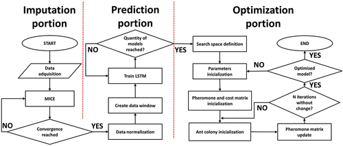
The proposed methodology consists in a preprocessing stage where missing data was imputed through the MICE algorithm and normalized through Equation (2)(2) $\frac{value-min}{max-min}$(2) . The prediction stage uses the predictive model described in Figure 8 which forecasts concentration 1 hr ahead. To prepare data for the optimization stage, a daily average of the predictions was obtained; this is due to the amount of data this algorithm receives as an input, where ants will generate an optimized model obtained through Equations (4(4) $y_{ij}=\left|\left(\frac{1}{n}x\sum _{i=1}^n{x}_{ij}\right)-x_{ij}\right|$(4) )–(9(9) $P_{ij}=\frac{{\left({\tau }_{ij}\right)}^{\alpha }{\left({\eta }_{ij}\right)}^{\beta }}{\sum {\left({\tau }_{ij}\right)}^{\alpha }{\left({\eta }_{ij}\right)}^{\beta }}$(9) ).

A flowchart of the entire methodology is shown in Figure 9. The preprocessing and prediction stages are covered in greater detail in (Ramírez-Montañez et al. 2019).

Figure 9. Proposed methodology.

Parameter definition

For the ACO algorithm to construct a variety of solutions, a fairly wide search space needs to be defined. This search space needs to be wide enough for the ants to construct a variety of solutions but not so wide that they would never converge to some solution.

The decision of how many LSTM models would define the search space was taken based on the experimentation shown in Figure 10 where the quantity of LSTM constructing the search space was being incremented 1 by 1 to see where the inflection point (optimal quantity of models) is located.

Figure 10. RMSE improvement percentage vs. number of LSTM models that compose the search space.

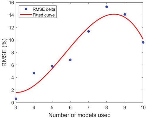
The PM10 data obtained from the Merced station was used for the experiment described in Figure 10 due to its low percentage of missing data, the lowest between stations and particles. As shown in the third degree polynomial fit in Figure 10, a clear inflection point can be observed at approximately 8 models defining the search space. Based on this experiment, all search spaces defined in this work will be constructed by 8 LSTM models.

Once the quantity of LSTM models was defined, the next stage consists of an experiment to determine the best combination of parameters for the ACO algorithm was developed. The definition of efficiency considered in the experiment was to reach the least RMSE difference between the obtained model and the imputed data using the least amount of time. This experiment was repeated 25 times to observe repeatability through the standard deviation of the RMSE results per combination of parameters; each of the results is shown in Table 2. This testing consisted in combining values for the number of ants (g in Equation (8)(8) ${\tau }_{ij}=\left(1-\rho \right){\tau }_{ij}+\sum _{f=1}^g\mathrm{\Delta }{\tau }_{ij}^f$(8) ) in the algorithm and for the evaporation rate (ρ in Equation (8)(8) ${\tau }_{ij}=\left(1-\rho \right){\tau }_{ij}+\sum _{f=1}^g\mathrm{\Delta }{\tau }_{ij}^f$(8) ). The weight of the pheromone concentration (α in Equation (9)(9) $P_{ij}=\frac{{\left({\tau }_{ij}\right)}^{\alpha }{\left({\eta }_{ij}\right)}^{\beta }}{\sum {\left({\tau }_{ij}\right)}^{\alpha }{\left({\eta }_{ij}\right)}^{\beta }}$(9) ) and the weight of feasibility (β in Equation (9)(9) $P_{ij}=\frac{{\left({\tau }_{ij}\right)}^{\alpha }{\left({\eta }_{ij}\right)}^{\beta }}{\sum {\left({\tau }_{ij}\right)}^{\alpha }{\left({\eta }_{ij}\right)}^{\beta }}$(9) ) were defined to be 1 in order to avoid any bias for the parameter initialization. The results considering a quantity of ants of 1, 3, 5,10, 25, and 50, and the evaporation rate of 0.1%,1%,5%, 10%, and 20% are shown in Table 2, this testing was developed using PM10 data of station in Xalostoc.

The termination criteria for the algorithm considered the ants to reach 25 iterations without finding a better solution than the local best.

Results in Table 2 presented ρ = 10% and ants = 5 as the most efficient combination of parameters show the lowest RMSE, 5.46, having a low amount of time, 3.41 sec. The repeatability of this combination of parameters is considered as high as the standard deviation of the 25 RMSEs obtained is 0.03. This experimentation demonstrates that a better result, in this case, not necessarily corresponds to a greater number of ants, but it seems that a greater evaporation rate is directly related to execution time. The challenge here was to find a combination of parameters that got the best results with high repeatability in the least amount of time. It seems important to note that RMSE seems very insensitive to these hyper parameters and standard deviation being practically 0 in all iterations. One possible explanation for this high repeatability and RMSE’s behavior is that the cost function allows the ACO algorithm to always converge around the same point due to its low complexity.

Evaluation

To evaluate the MICE algorithm, the standard deviation was calculated for the imputed and raw database using Equation (1)(1) $Std.Dev.=\sqrt{\frac{\sum _{i=1}^n{\left(xi-\bar{x}\right)}^2}{n-1}}$(1) .

To evaluate the optimized LSTM-ACO model, the RMSE, MAE, and the coefficient of determination were implemented; it is important to note that when evaluating the RMSE and MAE the lower the value the better (Wang and Lu 2018), and when evaluating the coefficient of determination, the higher the value the better (Zhang 2016). The purpose of these evaluations is to make a comparison between the resulting LSTMACO model and the mean of the measurements between the n LSTM models trained for each station for both PM_2.5 and PM_10.

The RMSE represents the standard deviation between actual and predicted values as Equation (10)(10) $RMSE=\sqrt{\frac{1}{n}\sum _{i=1}^n{\left(Y{M}_i-Y{R}_i\right)}^2}$(10) describes:

(10) $RMSE=\sqrt{\frac{1}{n}\sum _{i=1}^n{\left(Y{M}_i-Y{R}_i\right)}^2}$(10)

where YM_i refers to the i-th element of the prediction model and YR_i refers to the i-th element of the real data.

RMSE is a representation of how close the distance between the prediction and real values is. This value will be used to decide the optimal number of LSTM models to use as the search space in the ACO algorithm.

In order to evaluate the precision of the model obtained, the MAE was implemented using Equation (11)(11) $MAE=\frac{1}{n}\sum _{i=1}^n\left|Y{M}_i-Y{R}_i\right|$(11) :

(11) $MAE=\frac{1}{n}\sum _{i=1}^n\left|Y{M}_i-Y{R}_i\right|$(11)

Where YM_i refers to the i-th element of the prediction model and YR_i refers to the i-th element of the real data.

To evaluate how strong is the relationship between the predicted model and the real data, the correlation coefficient was implemented. The correlation coefficient’s values may vary between −1, a perfect negative correlation between data sets, and 1, a perfect correlation between data sets. The correlation coefficient (r) was implemented using Equation (12)(12) $r=\frac{n\left(\sum _{i=1}^n\left(Y{M}_i\right)\left(Y{R}_i\right)\right)-\left(\sum _{i=1}^{n}Y{M}_i\right)\left(\sum _{i=1}^{n}Y{R}_i\right)}{\sqrt{\left[n\sum _{i=1}^{n}Y{M}_i^2-\left(\sum _{i=1}^{n}Y{M}_i^2\right)\right]-\left[n\sum _{i=1}^{n}Y{R}_i^2-\left(\sum _{i=1}^{n}Y{R}_i^2\right)\right]}}$(12) :

(12) $r=\frac{n\left(\sum _{i=1}^n\left(Y{M}_i\right)\left(Y{R}_i\right)\right)-\left(\sum _{i=1}^{n}Y{M}_i\right)\left(\sum _{i=1}^{n}Y{R}_i\right)}{\sqrt{\left[n\sum _{i=1}^{n}Y{M}_i^2-\left(\sum _{i=1}^{n}Y{M}_i^2\right)\right]-\left[n\sum _{i=1}^{n}Y{R}_i^2-\left(\sum _{i=1}^{n}Y{R}_i^2\right)\right]}}$(12)

Where YM_i refers to the i-th element of the prediction model and YR_i refers to the i-th element of the real data.

In order to explain how much variability of one factor can be caused by its relationship to another factor, the coefficient of determination was implemented (r²) which is calculated by squaring the correlation coefficient.

The LSTM-ACO model was built by the ACO algorithm with the characteristics mentioned above using the 8 LSTM models as the ant’s search space and minimizing the cost in Equation (4)(4) $y_{ij}=\left|\left(\frac{1}{n}x\sum _{i=1}^n{x}_{ij}\right)-x_{ij}\right|$(4) . This is why it is necessary to compare the results for the LSTM models and the results for the LSTM-ACO models. The results shown are taken by Equation (13)(13) $delta=(\frac{Optimizedvalue-Initialvalue}{Initalvalue})x100$(13) :

(13) $delta=(\frac{Optimizedvalue-Initialvalue}{Initalvalue})x100$(13)

Where the optimized value refers to the LSTM-ACO model mean result and the initial value refers to the LSTM model mean result.

Results and discussion

The relationship between the percentage of the initial missing data (obtained in Table 1) in the database and the percentage difference between the mean of the imputed database and the mean of the initial database is shown in Figure 11a and the relationship between the percentage of the initial missing data in the database and the percentage difference between the standard deviation of the imputed database and the standard deviation of the initial database is shown in Figure 11b.

Figure 11. Relationship between initial missing data in set and the absolute difference of mean after imputation was implemented.

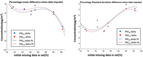
As shown in the third degree polynomial fits in Figure 11a, the trend in the relationship between initial missing data in set and the percentage difference of mean after imputation is negatively exponential according to the results obtained. This seems to indicate that the greater the percentage of missing data in databases is considered, less reliable the model will be related to the real PMx concentration in the area evaluated. Conversely, the highest difference presented in this work being the case of PM_2.5 in SAG station only presented a decrease of −5.48% in its mean. As shown in the third degree polynomial fits in Figure 11b, the trend in the relationship between the initial missing data in set and the absolute difference of standard deviation after imputation shows another behavior than the trend obtained in Figure 11a, standard deviation seems oscillate around the horizontal axis approximately in the 1.5% value. The case of PM10 for CAM station is shown as the highest difference in the standard deviation after imputed but only presented a rise of 3.83% in its standard deviation.

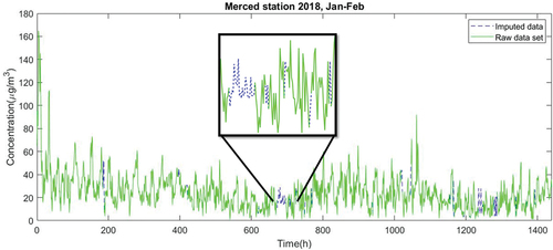
An example of how the MICE algorithm imputed the database is shown in Figure 12, showing the case of the Merced station between January and February of 2018.

Figure 12. Example of how MICE algorithm imputes the databases.

To avoid over-fitting, the models were trained with 80% percent of the imputed data and used the remaining 20% to forecast and evaluate the models. Eight models were obtained from the LSTM network, and using these 8 models as search space, 25 models were obtained through the ACO algorithm. These resulting models are going to be used for comparison in performance through RMSE in Equation (10)(10) $RMSE=\sqrt{\frac{1}{n}\sum _{i=1}^n{\left(Y{M}_i-Y{R}_i\right)}^2}$(10) , MAE in Equation (11)(11) $MAE=\frac{1}{n}\sum _{i=1}^n\left|Y{M}_i-Y{R}_i\right|$(11) and correlation coefficient squaring the obtained in Equation (12)(12) $r=\frac{n\left(\sum _{i=1}^n\left(Y{M}_i\right)\left(Y{R}_i\right)\right)-\left(\sum _{i=1}^{n}Y{M}_i\right)\left(\sum _{i=1}^{n}Y{R}_i\right)}{\sqrt{\left[n\sum _{i=1}^{n}Y{M}_i^2-\left(\sum _{i=1}^{n}Y{M}_i^2\right)\right]-\left[n\sum _{i=1}^{n}Y{R}_i^2-\left(\sum _{i=1}^{n}Y{R}_i^2\right)\right]}}$(12) . To evaluate the repeatability of the LSTM and LSTM-ACO models, the median, the standard deviation in Equation (1)(1) $Std.Dev.=\sqrt{\frac{\sum _{i=1}^n{\left(xi-\bar{x}\right)}^2}{n-1}}$(1) , and mean for each of the evaluation metrics that were obtained; to compare these results, a delta will be calculated with Equation (13)(13) $delta=(\frac{Optimizedvalue-Initialvalue}{Initalvalue})x100$(13) . The results of the predicted PM₁₀ RMSE for the 25 LSTM-ACO models and the RMSE of the 8 LSTM models are shown in Figure 13. The RMSE presented by the LSTM models presented a standard deviation of 1.16 for XAL, 0.84 for TLA, 0.77 for CAM, 0.41 for HGM, 1.87 for MER, and 1.49 for SAG, which was improved by the results obtained in this contribution by 97.01% for XAL, 99.48% for TLA, 99.71% for CAM, 97.35% for HGM, 99.55% for MER, and 99.13% for SAG. The RMSE presented by the LSTM models presented a mean of 6.44 for XAL, 3.93 for TLA, 4.38 for CAM, 3.12 for HGM, 4.46 for MER, and 5.91 for SAG, which was improved by the results obtained in this contribution by 15.17% for XAL, 5.17% for TLA, 34.62% for CAM, 9.23% for HGM, 18.66% for MER, and 8.34% for SAG. The results of the predicted PM_2.5 RMSE for the 25 LSTM-ACO models and the

Figure 13. PM₁₀ RMSE of LSTM models and LSTM-ACO models.

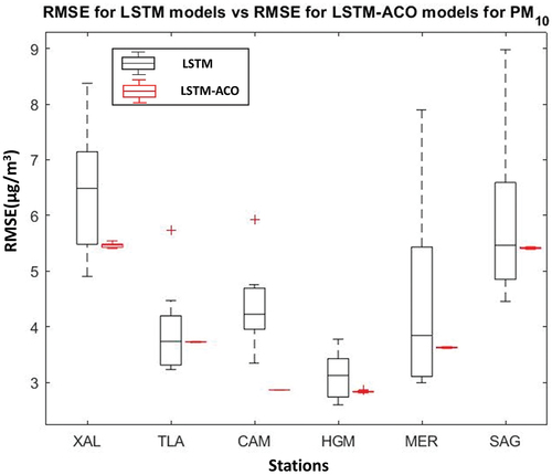
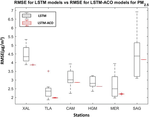
RMSE of the 8 LSTM models are shown in Figure 14. The RMSE presented by the LSTM models presented a standard deviation of 0.53 for XAL, 0.51 for TLA, 0.56 for CAM, 0.33 for HGM, 0.73 for MER, and 1.32 for SAG, which was improved by the results obtained in this contribution by 99% for XAL, 97.41% for TLA, 99.61% for CAM, 99.85% for HGM, 98.98% for MER, and 99.9% for SAG. The RMSE presented by the LSTM models presented a mean of 4.48 for XAL, 2.41 for TLA, 3.11 for CAM, 2.86 for HGM, 2.68 for MER, and 4.43 for SAG, which was improved by the results obtained in this contribution by 13.58% for XAL, 18.17% for TLA, 8.07% for CAM, 8.2% for HGM, 17.99% for MER, and 5.83% for SAG.

Figure 14. PM_2.5 RMSE of LSTM models and LSTM-ACO models.

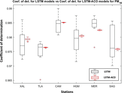
The results of the predicted PM₁₀ Coefficient of determination for the 25 LSTMACO models and the Coefficient of determination of the 8 LSTM models are shown in Figure 15. The coefficient of determination presented by the LSTM models presented a standard deviation of 0.005 for XAL, 0.004 for TLA, 0.003 for CAM, 0.005 for HGM, 0.003 for MER, and 0.006 for SAG, which was improved by the results obtained in this contribution by 91.5% for XAL, 97.64% for TLA, 98.13% for CAM, 95.63% for HGM, 95.67% for MER, and 96.84% for SAG. The coefficient of determination presented by the LSTM models presented a mean of 0.977 for XAL, 0.974 for TLA, 0.984 for CAM, 0.979 for HGM, 0.984 for MER, and 0.978 for SAG, which was improved by the results obtained in this contribution by −0.002% for XAL, −0.002% for TLA, −0.001% for CAM, −0.001% for HGM, 0.002% for MER, and 0.002% for SAG. Note that for the coefficient of determination a higher value is classified as a better fit.

Figure 15. PM₁₀ coefficient of determination of LSTM models and LSTM-ACO models.

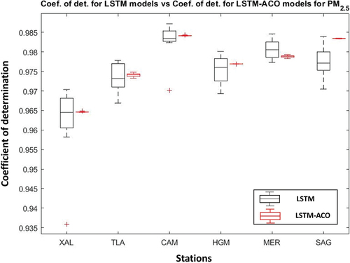
The results of the predicted PM_2.5 Coefficient of determination for the 25 LSTM-ACO models and the Coefficient of determination of the 8 LSTM models are shown in Figure 16. The Coefficient of determination presented by the LSTM models presented a standard deviation of 0.011 for XAL, 0.004 for TLA, 0.005 for CAM, 0.004 for HGM, 0.003 for MER, and 0.004 for SAG, which was improved by the results obtained in this contribution by 99.29% for XAL, 88.79% for TLA, 98.81% for CAM, 99.3% for HGM, 89.54% for MER, and 98.81% for SAG. The Coefficient of determination presented by the LSTM models presented a mean of 0.962 for XAL, 0.973 for TLA, 0.983 for CAM, 0.975 for HGM, 0.981 for MER, and 0.977 for SAG, which was improved by the results obtained in this contribution by −0.003% for XAL, −0.001% for TLA, −0.002% for CAM, −0.002% for HGM, 0.002% for MER, and −0.006% for SAG.

Figure 16. PM_2.5 coefficient of determination of LSTM models and LSTM-ACO models.

As seen in Figures 13–16, the proposed methodology presents a better result when evaluating with RMSE and MAE and for most cases, the coefficient of determination show much better results regarding responsibility, making this methodology an improvement when forecasting in no real-time PMx and highly reliable. The synthesized results for the LSTM models obtained for PM₁₀ and PM_2.5 are shown in Tables 3 and 4, respectively. These results include mean RMSE and its standard deviation, mean MAE and its standard deviation, and mean coefficient of determination and its standard deviation for the six stations evaluated.

Table 3. Evaluation metrics of LSTM models predicting PM₁₀ concentrations.

Stations	RMSE (µg/m^3)		MAE (µg/m^3)		Coef. of det.
	Mean	Std. Dev.	Mean	Std. Dev.	Mean	Std. Dev.
SAG	5.91	1.49	4.62	1.55	0.978	0.006
TLA	3.93	0.84	3.18	0.81	0.974	0.004
MER	4.46	0.19	3.72	1.98	0.984	0.003
XAL	6.44	1.16	5.11	1.01	0.977	0.005
HGM	3.12	0.41	2.41	0.37	0.979	0.005
CAM	4.38	0.77	3.42	0.73	0.984	0.003

Table 4. Evaluation metrics of LSTM models predicting PM_2.5 concentrations.

Stations	RMSE (µg/m^3)		MAE (µg/m^3)		Coef. of det.
	Mean	Std. Dev.	Mean	Std. Dev.	Mean	Std.Dev.
SAG	4.43	1.32	3.71	1.33	0.977	0.004
TLA	2.41	0.51	1.95	0.48	0.973	0.004
MER	2.68	0.73	2.15	0.76	0.981	0.003
XAL	4.48	0.53	3.52	0.59	0.962	0.011
HGM	2.86	0.33	2.23	0.36	0.975	0.004
CAM	3.11	0.56	2.39	0.46	0.983	0.005

The synthesized results for the LSTM-ACO models obtained for PM₁₀ and PM_2.5 are shown in Tables 5 and 6 respectively. These results include mean RMSE and its standard deviation, mean MAE and its standard deviation, and mean coefficient of determination and its standard deviation for the six stations evaluated.

Table 5. Evaluation metrics of LSTM-ACO models predicting PM₁₀ concentrations.

Station	RMSE	Std. Dev	MAE	Std. Dev.	Coef. of det.	Std. Dev.
SAG	5.41	0.01	4.30	0.02	0.976	0.000
TLA	3.72	0.00	3.00	0.01	0.976	0.000
MER	3.62	0.01	2.96	0.01	0.982	0.000
XAL	5.46	0.03	4.26	0.02	0.979	0.000
HGM	2.83	0.01	2.12	0.01	0.980	0.000
CAM	2.86	0.00	3.08	0.01	0.985	0.000

Table 6. Evaluation metrics of LSTM-ACO models predicting PM_2.5 concentrations.

Station	RMSE	Std. Dev.	MAE	Std. Dev.	Coef. of det	Std. Dev.
SAG	4.18	0.00	3.31	0.00	0.983	0.000
TLA	1.98	0.01	1.59	0.01	0.974	0.000
MER	2.19	0.01	1.69	0.00	0.979	0.000
XAL	3.87	0.01	2.93	0.00	0.965	0.000
HGM	2.63	0.00	1.99	0.00	0.977	0.000
CAM	2.86	0.00	2.13	0.00	0.984	0.000

It is worth highlighting the standard deviation results shown in Tables 5 and 6 where in all of the cases the standard deviation represents less than 1% of the evaluation metric being evaluated. Having no cases of outliers in Tables 5 and 6, the convergence of the LSTM-ACO models can be insured. These results may be translated to very robust models with high replicability of both PM_2.5 and PM₁₀.

Conclusion

In the present work, a novel methodology was proposed, consisting on taking raw PMx data, then filing the missing values using MICE imputation. Based on these imputed data, the data is trained in order to obtain a series of LSTM models and finally improve the predicted PMx concentrations of the recurrent network using the Ant Colony Algorithm. The proposed LSTM-ACO model was tested through various evaluation metrics that demonstrated high repeatability and a very high correlation with the original PMx databases obtaining in every scenario a better lower RMSE and MAE compared with the LSTM network and a coefficient of determination of 0.976 taking into consideration the 6 stations for both PM₁₀ and PM_2.5. These results seem to indicate a highly reliable and generalized model to predict PMx concentrations.

For future work, it may be pertinent to apply this methodology to different sequential (time-dependent) phenomena, and there is no need to respond in real time and evaluate their results.

Disclosure statement

No potential conflict of interest was reported by the author(s).

Data availability statement

The data that support the findings of this study are available in Partículas Suspendidas at http://www.aire.cdmx.gob.mx/default.php?opc=%27aKBhnmE=%27&r=b3Blb mRhdGEvcmVkX21hbnVhbC9yZWRfbWFudWFsX3BhcnRpY3VsYXNfc3VzcC5jc 3Y=, reference number n/a. These data were derived from the following resources available in the public domain: http://www.aire.cdmx.gob.mx/default.php?opc=%27ZaBhnmI=%27#:~:text=La%20Red%20Autom%C3%A1tica%20de%20Monitoreo,de%20los%20equipos%20de%20monitoreo.

Additional information

Notes on contributors

Gerardo Javier Kuri-Monge

Gerardo Javier Kuri-Monge received his B.SC. Degree in El Salvador and his M.SC. (Eng) in Artificial Intelligence at Universidad Autonoma de Queretaro, Mexico in 2022 with honors.

Marco Antonio Aceves-Fernández

Marco Antonio Aceves-Fernández received the B.Sc. degree in telematics engineering from Colima University, Mexico, and the M.Sc. and Ph.D. degrees in the field of intelligent systems from the University of Liverpool, U.K. He is a full-time Professor with the Engineering Faculty, Autonomous University of Querétaro, Mexico. His research interest includes intelligent and embedded systems. He has been a member of the National Systems of Researchers (SNI), since 2009. He is also the Honorary President of the Mexican Association of Embedded Systems (AMESE) and a Board Member for many Institutions and Associations.

Jesús Carlos Pedraza-Ortega

Jesús Carlos Pedraza-Ortega received the B.Sc. degree in electronics engineering from the Celaya Institute of Technology, Mexico, the M.Sc. degree in electrical engineering from the FIMEE Universidad de Guanajuato, and the Ph.D. degree in mechanical engineering from the University of Tsukuba, Japan. He is a full-time Professor with the Engineering Faculty, Autonomous University of Querétaro, Mexico. He has been a member of the National Systems of Researchers (SNI), since 2004, and the Mexican Science Academy (AMC), since 2007. His research interests include machine vision, 3D reconstruction, image processing, and deep and machine learning.

References

- Aceves, M., R. Domínguez, J. Pedraza, and J. E. Vargas-Soto. 2020. Evaluation of key parameters using deep convolutional neural networks for airborne pollution (PM10) prediction. Discrete Dyn. Nat. Soc 2020:1–14. doi:10.1155/2020/2792481.
- Becerra, J., M. Aceves, K. Esquivel, and J. C. Pedraza-Ortega. 2020. Airborne particle pollution predictive model using Gated Recurrent Unit (GRU) deep neural networks. Earth Sci. Inf 13(3):821–34. doi:10.1007/s12145-020-00462-9.
- Beesley, L., and J. Taylor. 2019. A stacked approach for chained equations multiple imputation incorporating the substantive model. Biometrics doi:10.1111/biom.13372.
- Beni, G., and J. Wang. 1993. Swarm Intelligence in Cellular Robotic Systems. In Robots and Biological Systems: Towards a New Bionics?, ed. P. Dario, G. Sandini, and P. Aebischer, vol. 102. Berlin, Heidelberg: Springer. https://doi.org/10.1007/978-3-642-58069-7_38.
- Bodor, K., M. Micheu, A. Keresztesi M. V. Birsan, I. A. Nita, Z. Bodor, S. Petres, A. Korodi, and R. Szep. 2021. Effects of PM10 and weather on respiratory and cardiovascular diseases in the Ciuc basin. Atmosphere 12(2):289–310. doi:10.3390/atmos12020289.
- Cabrera, M., M. Aceves, J. Ramos, J. M. Ramos-Arreguin, J. E. Vargas-Soto, and E. Gorrostieta-Hurtado. 2019. Parameters influencing the optimization process in airborne particles PM10 using a neuro-fuzzy algorithm optimized with bacteria foraging. Int. J. Intell. Sci 9(3):67–91. doi:10.4236/ijis.2019.93005.
- Chakraborty, A., and A. Kar. 2017. Swarm intelligence: A review of algorithms. Nature-inspired computing and optimization 10:479–94. doi:10.1007/978-3-319-50920-4_19.
- Chen, K., Y. Zhou, and F. Dai. 2015. A LSTM-based method for stock returns prediction: A case study of China stock market. International Conference on Big Data, 2823–24.
- Cheng, J., G. Zhang, Z. Li, and Y. Li. 2011. Multi-objective ant colony optimization based on decomposition for bi-objective traveling salesman problem. Soft Comput 16(4):597–614. doi:10.1007/s00500-011-0759-3.
- Christidis, T., A. Erickson, A. Pappin, D. L. Crouse, L. L. Pinault, S. A. Weichenthal, J. R. Brook, A. van Donkelaar, P. Hystad, R. V. Martin, and M. Tjepkema. 2019. Low concentrations of fine particle air pollution and mortality in the Canadian Community Health Survey cohort. Environ. Health 18(84):1–16. doi:10.1186/s12940-019-0518-y.
- de Ecología IN. 2019. Manual 2: Sistemas de Medición de la Calidad del Aire. March. https://sinaica.inecc.gob.mx/archivo/guias/2/%20-/%20Sistemas/%20de/%20Medici/%C3/%B3n/%20de/%20la/%20Calidad/%20del/%20Aire.pdf.
- Deng, W., J. Xu, and X. Zhao. 2019. An improved ant colony optimization algorithm based on hybrid strategies for scheduling problem. IEEE Access 7. doi:10.1109/ACCESS.2019.2897580.
- Dorigo, M., V. Maniezzo, and A. Coloni. 1996. Ant system: Optimization by a colony of cooperating agents. Trans. Syst. Man Cybern 26 (1):29–41. doi:10.1109/3477.484436.
- Dorigo, M., and T. Stützle. 2010. Ant colony optimization: Overview and recent advances. Int. Ser. Oper. Res. Manage. Sci 272:311–51. doi:10.1007/978-1-4419-1665-5-8.
- Faris, H., A. Al-Zoubi, A. Heidari, I. Aljarah, M. Mafarja, M. A. Hassonah, and H. Fujita. 2019. An intelligent system for spam detection and identification of the most relevant features based on evolutionary random weight networks. Inf. Fusion 48:67–83. doi:10.1016/j.inffus.2018.08.002.
- Ghosh, M., R. Guha, R. Sarkar, and A. Abraham. 2019. A wrapper-filter feature selection technique based on ant colony optimization. Neural Comput. Appl doi:10.1007/s00521-019-04171-3.
- Government MC. 2021. Air quality monitoring. http://www.aire.cdmx.gob.mx/default.php?opc=/%27ZaBhnmI=/%27.
- Gu, F., B. Ma, J. Guo, P. A. Summers, and P. Hall. 2017. Internet of things and big data as potential solutions to the problems in waste electrical and electronic equipment management: An exploratory study. Waste Manage 68:434–48. doi:10.1016/j.wasman.2017.07.037.
- Hochreiter, S., and J. Schmidhuber. 1997. Long short-term memory. Neural Comput 9 (8):1735–80. doi:10.1162/neco.1997.9.8.1735.
- Hua, Y., R. Z. Zhao, R. Li, X. Chen, Z. Liu, and H. Zhang. 2019. Deep learning with long short-term memory for time series prediction. Internet Things Sendor Network. doi:10.1109/MCOM.2019.1800155.
- Ismkhan, H. 2017. Effective heuristics for ant colony optimization to handle large-scale problems. Swarm Evol. Comput 32:140–49. doi:10.1016/j.swevo.2016.06.006.
- Klambauer, G., T. Unterthiner, and A. Mayr. 2017. Self-normalizing neural networks. Comput. Sci 3. Available from. doi:10.48550/arXiv.1706.02515.
- Kumar, A., P. Dash, R. Dash, and R. Bisoi. 2017. Forecasting financial time series using a low complexity recurrent neural network and evolutionary learning approach. J. King Saud Univ. Comput. Inf. Sci 29(4):536–52. doi:10.1016/j.jksuci.2015.06.002.
- Lee, B., B. Kim, and K. Lee. 2014. Air pollution exposure and cardiovascular disease. Toxicol. Res 30(2):71–75. doi:10.5487/tr.2014.30.2.071.
- Li, Y., H. Soleimani, and M. Zohal. 2019. An improved ant colony optimization algorithm for the multidepot green vehicle routing problem with multiple objectives. J. Clean. Prod 227:1161–72. doi:10.1016/j.jclepro.2019.03.185.
- Liu, Y., C. Yang, C. Wu, Q. D. Sun and W. Bi. 2019. Threshold changeable secret image sharing scheme based on interpolation polynomial. Multimed. Tools Appl 78(13):18653–67. doi:10.1007/s11042-019-7205-4.
- Mu, H., S. Otani, M. Okamoto, Y. Yokoyama, Y. Tokushima, K. Onishi, T. Hosoda and Y. Kurozawa. 2014. Assessment of effects of air pollution on daily outpatient visits using the air quality index. J. Med. Sci 57 (4):133–36.
- Nguyen, B., B. Xue, and M. Zhang. 2020. A survey on swarm intelligence approaches to feature selection in data mining. Swarm Evol. Comput 54:100663. doi:10.1016/j.swevo.2020.100663.
- Nikoonahad, A., R. Naserifar, V. Alipour, Poursafar, A., Miri, M.,Ghafari, H. R., and A. Mohammadi. 2017. Assessment of hospitalization and mortality from exposure to PM10 using AirQ modeling in Ilam, Iran. Environ. Sci. Pollut. Res 24 (27):21791–96. doi:10.1007/s11356-017-9794-7.
- Ning, J., Q. Zhang, C. Zhang, and B. Zhang. 2018. A best-path-updating information-guided ant colony optimization algorithm. Inf. Sci 433(434):142–62. doi:10.1016/j.ins.2017.12.047.
- Ordeñez, B., M. Aceves, S. Fernández, J. M. Ramos-Arreguín, and E. Gorrostieta-Hurtado. 2019. An improved particle swarm optimization (PSO): method to enhance modelling of airborne particulate matter (PM10). Evolving Syst 11(4):615–24. doi:10.1007/s12530-019-09263-y.
- Paniri, M., M. Bagher, and H. Nezamabadi-pour. 2020. Ant colony optimization for multi-objective optimization problems. Knowledge-Based Syst 192(15). doi:10.1016/j.knosys.2019.105285.
- Pérez-Cirera, V., E. Schmelkes, O. López-Corona, F. Carrera, A. P. García-Teruel and G. Teruel. 2016. Ingreso y calidad del aire en ciudades: ¿Existe una curva de Kuznets para las emisiones del transporte en la Zona Metropolitana del Valle de Mexico? El trimestre económico 85(340):745–764.
- Prokuryakov, A. 2017. Intelligent system for time series forecating. Procedia Comput. Sci 103:363–69. doi:10.1016/j.procs.2017.01.122.
- RAMA. 2021. Databases automatic air monitoring network. www.aire.cdmx.gob.mx/default.php?opc=/%27aKBh/%27.
- Ramírez-Montañez, J., M. A. Fernández, A. T. Arriaga, J. M. Arreguin and G. A. Calderon. 2019. Evaluation of a recurrent neural network LSTM for the detection of exceedances of particles PM10. International Conference on Electrical Engineering, Conputing Science and Automatic Control (CCE), Mexico City, Mexico, September 11–13.
- Resche-Rigon, M., and I. White. 2016. Multiple imputation by chained equations for systematically and sporadically missing multilevel data. Stat. Methods Med. Res 1–16. doi:10.1177/0962280216666564.
- Royston, P., and I. White. 2011. Multiple imputation by chained equations (MICE): Implementation in stata. J. Stat. Softw 45 (4). doi:10.18637/jss.v045.i04.
- Schranz, M., G. Di Caro, T. Schmickl, W. Elmenreich, F. Arvin, A. Şekercioğlu, and M. Sende. 2021. Swarm intelligence and cyber-physical systems: concepts, challenges and future trends. Swarm Evol. Comput 60:100762. https://doi.org/10.1016/j.swevo.2020.100762
- Sotomayor, A., M. Aceves, E. Gorrostieta, C. Pedraza-Ortega, J. M. Ramos-Arreguín, and J. E. Vargas-Soto. 2013. Forecast urban air pollution in Mexico city by using support vector machines: a kernel performance approach. Int. J. Intell. Sci 3(3):126–35. doi:10.4236/ijis.2013.33014.
- Tellez, M., D. López, and P. Fernández. 2018. La movilidad en la Ciudad de México: Impactos, conflictos y oportunidades. Academia 10:73–86.
- Uthayakumar, J., N. Metawa, K. Shankar, and S. K. Lakshmanaprabu. 2020. Financial crisis prediction model using ant colony optimization. Int. J. Inf. Manage 50:538–56. doi:10.1016/j.ijinfomgt.2018.12.001.
- Wang, H. Z., L. T. Xing, Y. Yang, R. Qu, and Y. Pan. 2016. A modified ant colony optimization algorithm for network coding resource minimization. IEEE Trans. Evol. Comput 20(3):325–42. doi:10.1109/TEVC.2015.2457437.
- Wang, W., and Y. Lu. 2018. Analysis of the Mean Absolute Error (MAE) and the Root Mean Square Error (RMSE) in assessing rounding model. IOP Conference Series: Materials Science and Engineering, Kuala Lumpur, Malasya. IOP Publishing.
- WHO. 2018. Ambient (outdoor) air quality and health. May.
- WHO. 2021. WHO air quality guidelines for particulate matter, ozone, nitrogen dioxide and sulfur dioxide, 6–10.
- Wulff, J., and L. Jeppesen. 2017. Multiple imputation by chained equations in praxis: Guidelines and review. Electron. J. Bus. Res. Methods 15 (1):41–56.
- Xu, S., Y. Liu, and M. Chen. 2017. Optimization of partial collaborative transportation scheduling in supply chain management with 3PL using ACO. Expert Syst. Appl 71:173–91. doi:10.1016/j.eswa.2016.11.016.
- Yan, Y., Y. Li, M. Sun and Z. Wu. 2019. Primary pollutants and air quality analysis for urban air in China: evidence from Shanghai. Sustainability 11(8):2319. doi:10.3390/su11082319.
- Yixiang, X., and Y. Chunning. 2020. Fault recognition of electric servo steering gear based on long and short-term memory neural network. International Conference on Unmanned Aircraft Systems (ICUAS), Athens, Greece, September. https://doi.org/10.1109/ICUAS48674.2020.9213882
- Zhang, D. 2016. A coefficient of determination for generalized linear models. Am. Stat 71 (4):310–16. doi:10.1080/00031305.2016.1256839.
- Zhao, D., L. Liu, F. Yu, A. A. Heidari, M. Wang, D. Oliva, K. Muhammad, and H. Chen. 2020. Ant colony optimization with horizontal and vertical crossover search: fundamental visions for multi-threshold image segmentation. Expert Syst. Appl 114122. doi: 10.1016/j.eswa.2020.114122.
- Zhu, B., S. Ma, R. Xie, J. Chevallier, and Y. M. Wei. 2018. Hilbert spectra and empirical mode decomposition: a multi-scale event analysis method to detect the impact of economic crises on the European carbon market. Comput. Econ 52(1):105–21. doi:10.1007/s10614-017-9664-x.