A fuzzy control algorithm for tracing air pollution based on unmanned aerial vehicles

ABSTRACT

The process of atmospheric pollutants traceability based on unmanned aerial vehicles (UAVs) is affected by many factors that can impact and increase the complexity of the traceability of atmospheric pollutants. In this study, we proposed a new algorithm called the fuzzy control traceability (FCT) to track odor plumes. Our proposed algorithm combined the characteristics and fuzzy control of the UAV and designed a controller based on the actual environment of the UAV. The fuzzy controller fuzzed the input gas concentration information, established fuzzy control rules by imitating human brain thinking, and outputted the turning angle and the move length according to rules, thus realizing intelligent tracking of the odor plume by the UAV. We compared the FCT algorithm with the bio-inspired “ZigZag” algorithm to validate its performance. Various concentration fields were constructed, and ten sets of experiments are performed using the two algorithms in different concentration fields. The average success rate of the FCT algorithm under different concentration fields was 95.4% higher than that of the ZigZag algorithm.

Implications: Fuzzy control logic is applied to the field of air pollutant traceability of drones, and a single drone traceability algorithm based on fuzzy control is proposed; and in view of the shortcomings of a single traceability subject in the traceability, multiple traceability subjects are introduced to optimize fuzzy control.

Introduction

With the advancement of industrialization, the problem of air pollution has intensified. Traditional pollution source locations generally use fixed monitoring stations, vehicle mounted monitoring stations, or wireless sensor networks (Jatmiko, Sekiyama, and Fukuda 2006; Longinus, John, and Olatunde et al. 2016; White et al. 2008). However, owing to the limitation of ground conditions, monitoring stations are often unevenly distributed, altogether absent, or they may be surrounded by detection stations near the accidental pollution sources. Although the quality of environmental monitoring can be improved by additional monitoring stations and observation frequency, issues with limited detection range, high cost, poor mobility are pervasive obstacles. Since the end of the last century, the industry has used mobile robots with gas sensors to search identify pollution sources in real time, commonly known as the active olfaction of robots (Meng and Li 2006). However, when mobile robots on the ground perform plume tracking, they often become trapped in the complex ground environment and thus are limited to the laboratory stage. The development of unmanned aerial vehicles (UAVs) has provided a new method for solving the problem of air pollution. At present, researchers mostly use UAVs to carry gas sensors for atmospheric monitoring; however, they rarely use UAVs to trace sources of air pollutants. Owing to their flexibility and wide monitoring range, UAVs hold great promise in the growing field of active olfactory smells, particularly when chemical plants emit undetected gaseous waste. UAVs can quickly locate discharge areas and solve potential pollution problems in time, ultimately benefitting the environment and human health.

The gases released by air pollution sources are manipulated by wind and temperature, forming a three-dimensional odor plume. As plumes move away from pollution sources, they are diluted by molecular diffusion and turbulence that mix the odor molecules with clean air. Therefore, addressing the issue of atmospheric pollutant tracing by UAV includes three successive stages: plume finding, plume traversal, and odor source declaration. This study, among many others, focused on the second phase, plume traversal. Under the experimental condition of constant airflow, the plume shape is relatively regular. However, under the condition of no wind or breeze, odor molecules are affected by gas turbulence and are not evenly distributed, so the traversal process is very complicated. Although international scholars have conducted substantial research on this issue, the traceability of pollution remains a difficult task.

At this stage, air pollutant traceability algorithms can generally be divided into four categories: probabilistic distribution-based traceability, formation-based traceability, map-based traceability, and bio-inspired traceability algorithm (Gideon and Russell et al. 2008). Probabilistic distribution-based traceability algorithms model the location of pollution sources as a probability distribution. A typical case is that Infotaxis uses the “information axis”, a non-gradient search algorithm to move the tracer subject toward the location that maximizes information gain (Vergassola, Villermaux, and Shraiman 2007). However, in the calculation process, all data on time are included in the algorithm, thus as time progresses, this algorithm will still use the relatively old data which makes it less reliable.

The formation-based traceability algorithm involves requires at least two tracing subjects to interact with each other; however, the control technology of group intelligence is not mature enough at present and lacks an efficient interactive influence on the success rate of tracing (Demetriou, Egorova, and Gatsonis 2016; Fu, Chen, and Ding et al. 2019; Gu et al. 2018; Park and Oh 2020).

The map-based algorithm constructs a gas concentration map of the search area rather than directly searching for pollution sources (Kowadlo and Russell 2009; Qiu, Chen, and Wang et al. 2017). There are also overlaps with the probabilistic distribution-based traceability algorithm. Moreover, unstable gas diffusion may lead to inconsistencies in the constructed gas concentration diagram, which may then require more complex algorithms to solve.

The bio-inspired traceability algorithm derives inspiration from biology of certain species and traditionally combines chemotaxis and anti-chemotaxis (Fu, Shen, and Liu 2021; Lochmatter 2010; Lu, Zhang, and Li 2010; Zhang, Zhang, and Meng et al. 2008). For examples, in 1992, Ishida et al. at The Tokyo Institute of Technology in Japan studied the mate location strategy of male moths using olfactory information to find females ultimately proposing a concentration gradient algorithm and a headwind search algorithm (Ishida et al. 1994; Lochmatter 2010). In 1998, Professor Russell et al. developed a six-legged ant smell robot. Russell studied the behavior of ants using their head antennae as olfactory organs in the foraging process and proposed an algorithm for locating a smell source in the semi-circular eight-shape path of the smell robot (Russell 1999, 2004a, 2004b; Russell et al. 2003). Through the improvement of neural networks, the Li Yongming team applied an adaptive neural network to finite time optimal control, which can ensure the stability of the system and minimize the cost function; however, this innovation is still in the theoretical stage (Li, Li, and Tong 2020; Li, Yang, and Tong 2020). Most of these algorithms require the tracer to react in time, which means that the tracer only considers the current (or very recent) gas state of the concentration field. Therefore, this kind of algorithm has a low requirement for computing resources so that the traceability subject can respond quickly, similar to the algorithm used in this study.

Unlike the above bio-inspired traceability algorithms, the fuzzy control traceability (FCT) algorithm does not directly derive inspiration from a particular species but rather attempts to reproduce the multi-scale observations of various species. Fuzzy control is an intelligent control method based on the concepts of fuzzy mathematics (Cheng, Feng, and Lv 2012; Hu 2021). As a branch of artificial intelligence, fuzzy control is widely used in various fields, but it has rarely been used in the field of atmospheric traceability. Fuzzy control has since been applying to the field of active olfactory study, and the combination of its own robustness and “perceptual action behavior” based on physiology enhances the improvement of atmospheric traceability efficiency. A fuzzy controller can be designed to complete corresponding tasks without relying on the mathematical model of the object or on the information of the concentration gradient and wind direction, rather biological expertise is used to complete the corresponding tasks (Ge, Wang, and Wei et al. 2013; Li and Wang 2013). In addition, UAVs are is used as the carrier of the algorithm to identify, judge, and process gas concentration by imitating the thinking of the human brain, which can efficiently solve the traceability problem in unknown and complex environments. The effectiveness and feasibility of the algorithm were verified through simulations.

Herein, we aimed to establish a traceability simulation environment and traceability metrics based on fuzzy control. The results of simulation experiments conducted in different environments have been discussed in detail. With regards to the shortcomings of a single traceability subject, multiple traceability subjects are introduced to optimize the FCT algorithm, and finally, a refined multi-UAV traceability algorithm based on fuzzy control has been proposed.

Principle of fuzzy control algorithm

This chapter introduces the design of the fuzzy controller and defines its input and output membership functions. Simultaneously, the fuzzy rule table and reasoning are constructed, and the application of the fuzzy control traceability algorithm to gas traceability is explained in detail. Finally, this chapter introduces the layout of two types of pollution concentration scenarios, and presents the performance metrics of the evaluation algorithms.

Fuzzy controller design

In this study, the UAV used was idealized and regarded as a particle with no position deviation during its movement. It was able to turn 360° in situ regardless of the width required for its path or the space required for turning. The gas sensors were located in the front, back, left, and right directions of the UAV, and four gas concentration data can be obtained in one measurement. The UAV structure is diagrammed in Figure 1.

Figure 1. Schematic diagram of the UAV structure.

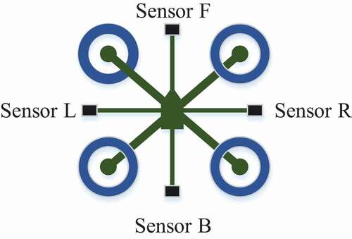
In the process of UAV traceability, the input of the controller was identified as the concentration of four gas sensors located in the front (F), back(B), left (L), and right (R) sections of the UAV. The output of the controller was defined as the move length and turning angle of the UAV, as shown in Figure 2.

Figure 2. The input-output relationship of the fuzzy controller.

Fuzzy measure

Membership function of input variables

The gas concentration range measured by the gas sensor was uniformly quantified into the interval [0, C], the domain of discussion was [0.1C, 0.5C, 0.9C], and the corresponding variable fuzzy language was C = {S, M, W} = {Strong, Medium, Weak}. The membership function formula is shown in formula (1), and the membership degree image considers the gas sensor (F) concentration in front of the UAV as an example, as shown in Figure 3.

Figure 3. Membership function of the input “Front”.

(1) $C_i=\left\{\begin{array}{c}{C}_i\mathrm{W}=\left\{\begin{array}{c}\begin{array}{cc}1& x\le 0.1\end{array}\\ \begin{array}{cc}\frac{0.5-x}{0.4}& 0.1<x\end{array}\le 0.5\end{array}\right.\\ C_i\mathrm{M}=\left\{\begin{array}{cc}\frac{x-0.1}{0.4}& 0.1<x\le 0.5\\ \frac{0.9-x}{0.4}& 0.5<x\le 0.9\end{array}\right.\\ C_i\mathrm{S}=\left\{\begin{array}{cc}\frac{x-0.5}{0.4}& 0.5<x\le 0.9\\ 1& x>0.9\end{array}\right.\end{array}\right.\begin{array}{cc}\hspace{0.17em}& i=\{F,B,L,R\}\end{array}$(1)

Membership function of output variables

By uniformly quantizing the output turning angle within the interval of [0°, 360°], the domain of discussion was [0°, 30°, 75°, 135°, 180°, 210°, 240°, 270°, 300°, 330°, 360°.] and Angle = {A1, A2, A3, A4, A5, A6, A7, A8, A9}. The membership degree image is shown in Figure 4.

Figure 4. Membership function of the output “Angle”.

The output move length was uniformly quantized into the interval [0,d], and the domain of discussion was [0,1d,√2d,√4d,√5d,√8d,√9d,√10d,√13d,√18d]. Step = {ST1, ST2, ST3, ST4, ST5, ST6, ST7}. The membership degree image of this output is shown in Figure 5.

Figure 5. Membership function of the output “Step”.

The minimum move length of the UAV is a standard unit Represented as d. The turning angle before each movement was vector synthesized according to the length of the front, back, left, and right sections of the UAV.

Constructing fuzzy rules and reasoning

Fuzzy rules

The premise of UAV traceability is to find the real source of pollution in the shortest time and distance. Each flight of the UAV moved toward of a higher gas concentration. The basic rules were established as follows:

(1) Establish a coordinate system based on the front, back, left, and right of the UAV, with the front direction oriented at 0°and the clockwise direction being positive.

(2) When there is a sensor with a concentration of S, the movement length is d. For example, the gas concentration in the front of the UAV is S, and the gas concentration in the back is W, so the movement length is d.

(3) When the gas concentrations of the front and back (left and right) sensors are M, the movement length is 2d. For example, if the gas concentration in front of the UAV is M, and the gas concentration in the back is W, so the move length of the forward walk is 2d.

(4) When the concentrations of the front and back (left and right) sensors are both W, the move length is 3d; For example, if the gas concentration in front of the UAV is W and the gas concentration in the back is W, the move length of the forward walk is 3d.

(5) When the concentrations of the front and back (left and right) sensors are the same, the UAV moved forward (left).

(6) When the front and back sensors were both S, no movement occurred in either the front or back directions. The same is true for the left and right sides.

(7) When the concentration of the front, back, left, and right gas sensors of the UAV is S, the source has been identified.

(8) When it is necessary to move forward (back) and left (right) simultaneously the vector synthesis principle is followed to obtain the move length and turning angle. For example, if the gas concentration at the front of the UAV is S, the gas concentration at the back is M, the gas concentration on the left is M, and the gas concentration on the right is W.

According to the above rules, the move length of the forward walk is d, and that of the left walk is 2d. According to the principle of vector synthesis, the UAV only needs to move√5d in the direction of 296.6°.

According to the input and output variables and the above basic principles, 3 × 3 × 3 × 3 = 81 fuzzy control rules in total can be established, as listed in Table 1.

Table 1. The fuzzy control rule.

F	B	L	R	ST&A
S	S	S	S	A1
S	S	S	M	ST1&A7
S	S	S	W	ST1&A7
S	S	M	S	ST1&A2
S	S	M	M	ST3&A7
S	S	M	W	ST3&A7
…	…	…	…	…
W	W	W	M	ST7&A1
W	W	W	W	ST7&A8

Fuzzy reasoning and defuzzification

In this study, the Mamdani reasoning method was used to substitute the gas concentration data output of the four gas sensors into the membership function of Equation (1)(1) $C_i=\left\{\begin{array}{c}{C}_i\mathrm{W}=\left\{\begin{array}{c}\begin{array}{cc}1& x\le 0.1\end{array}\\ \begin{array}{cc}\frac{0.5-x}{0.4}& 0.1<x\end{array}\le 0.5\end{array}\right.\\ C_i\mathrm{M}=\left\{\begin{array}{cc}\frac{x-0.1}{0.4}& 0.1<x\le 0.5\\ \frac{0.9-x}{0.4}& 0.5<x\le 0.9\end{array}\right.\\ C_i\mathrm{S}=\left\{\begin{array}{cc}\frac{x-0.5}{0.4}& 0.5<x\le 0.9\\ 1& x>0.9\end{array}\right.\end{array}\right.\begin{array}{cc}\hspace{0.17em}& i=\{F,B,L,R\}\end{array}$(1) . After obtaining the four input quantities, the fuzzy control rule table in Table 1 was used to determine the corresponding fuzzy rule. The premise of each rule is to use the relationship “and” to draw conclusions simultaneously. The method used for the credibility of the rule uses a small method for the output.

The clarification method adopts the center of gravity method. The obtained clarification value is transformed into the actual control amount by scale transformation. The center of gravity method considers the center of gravity of the area enclosed by the membership function curve and abscissa as the final output values of the fuzzy inference. The calculation method is Equation (2)(2) $v_0=\frac{\sum _{k=1}^m{v}_k{\mu }_v(v_k)}{\sum _{k=1}^m{\mu }_v(v_k)}$(2) :

(2) $v_0=\frac{\sum _{k=1}^m{v}_k{\mu }_v(v_k)}{\sum _{k=1}^m{\mu }_v(v_k)}$(2)

where, $v_k$ is the center of gravity value corresponding to each membership function of the output value, and ${\mu }_v(v_k)$ is the credibility corresponding to each output value.

Application analysis of the algorithm

Taking this design requirement as the background to analyze the calculation example, if the concentration in front of the UAV is 0.9, that in the back is 0.4, that in the left is 0.6, and that in the right of the UAV is 0.5. The concentration data is then substituted into the membership function of Equation (1)(1) $C_i=\left\{\begin{array}{c}{C}_i\mathrm{W}=\left\{\begin{array}{c}\begin{array}{cc}1& x\le 0.1\end{array}\\ \begin{array}{cc}\frac{0.5-x}{0.4}& 0.1<x\end{array}\le 0.5\end{array}\right.\\ C_i\mathrm{M}=\left\{\begin{array}{cc}\frac{x-0.1}{0.4}& 0.1<x\le 0.5\\ \frac{0.9-x}{0.4}& 0.5<x\le 0.9\end{array}\right.\\ C_i\mathrm{S}=\left\{\begin{array}{cc}\frac{x-0.5}{0.4}& 0.5<x\le 0.9\\ 1& x>0.9\end{array}\right.\end{array}\right.\begin{array}{cc}\hspace{0.17em}& i=\{F,B,L,R\}\end{array}$(1) .

The degree of membership with a strong concentration in front of the UAV is 1, that with a weak concentration on the back is 0.25, that with a medium concentration on the back is 0.75, that with a medium concentration on the left is 0.75, that with a strong concentration on the left is 0.25, and that with a medium concentration on the right is 1.

After substituting the above data into the fuzzy control rule table for the rule-matching search, the following four rules can be established:

(1) If (F is S) and (B is W) and (L is M) and (R is M), then (step is ST4) (angle is A8).

(2) If (F is S) and (B is W) and (L is S) and (R is M), then (step is ST2) (angle is A8).

(3) If (F is S) and (B is M) and (L is M) and (R is M), then (step is ST4) (angle is A8).

(4) If (F is S) and (B is M) and (L is S) and (R is M), then (step is ST2) (angle is A8).

The following are examples of Rule (1) and Rule (3):

In Rule (1), if the gas concentration in front of the UAV has a strong membership degree of C_FS (0.9) = 1, the gas concentration at the back of the UAV has a weak membership degree of C_BW (0.4) = 0.25, the gas concentration on the left of the UAV has a medium membership degree of C_LM (0.6) = 0.75, and the gas concentration on the right of the UAV has a medium membership degree of C_RM (0.5) = 1; thus, the credibility of this rule is described as min (1, 0.25, 0.75, 0.5) = 0.25.

In Rule (3), if the gas concentration in front of the UAV has a strong membership degree of C_FS (0.9) = 1, the gas concentration at the back of the UAV has a medium membership degree of C_BM (0.4) = 0.75, the gas concentration on the left of the UAV has a medium membership degree of C_LM (0.6) = 0.75, and the gas concentration on the right of the UAV has a medium membership degree of C_RM (0.5) = 1. Thus, the credibility of this rule is min (1, 0.75, 0.75, 1) = 0.75.

After obtaining the reliability of the UAV’s move length and turning angle under the above setting conditions, the fuzzy subset is defuzzified using the center of gravity method, and the reliability corresponding to each output value is substituted into Equation (2)(2) $v_0=\frac{\sum _{k=1}^m{v}_k{\mu }_v(v_k)}{\sum _{k=1}^m{\mu }_v(v_k)}$(2) , where the movement length of the UAV is 2d, and the turning angle is 300°.

When the UAV completes this move, it obtains new gas concentration data and a new fuzzy input value according to the algorithm, performs fuzzy reasoning and defuzzification, obtains the move length and turning angle of the next move, and controls the approach of the UAV until it finds the source of the pollution.

Pollutant concentration field

The traceability algorithm should be evaluated under various environmental conditions, thus designing an air pollutant diffusion concentration field for the traceability algorithm is necessary. Numerical simulations are a widely used scientific research method, as this method can not only fully and intuitively understand the diffusion law of atmospheric pollutants and air flow characteristics, but can also show different diffusion characteristics under different environmental conditions. Therefore, this study used numerical simulation to build an environment gradient of gas diffusion in an ideal environment and gas diffusion in a complex environment.

The Gaussian pollutant diffusion model was selected for a gas diffusion simulation in an ideal environment. The parameters of the Gaussian pollutant diffusion model(Table 2) was set as the length and width of the pollutant diffusion environment, 150 × 80 m; the coordinates of the air pollution source, (0 m, 20 m); the emission intensity of the pollution source Q = 1–10 g/s; the effective height of the pollution source, 1 m; and the diffusion coefficients in the y and z-axis directions are ${\sigma }_y=0.08x/{\left(1+0.0001x\right)}^{0.5}$ and ${\sigma }_z=0.06x/{\left(1+0.0001x\right)}^{0.5}$, respectively. A simulation example of the Gaussian pollutant diffusion model assuming that the average wind speed u is 0.5–1.0 m/s and that z = 1.5 m, is shown in Figure 6.

Figure 6. Pollutant diffusion simulation in an ideal environment.

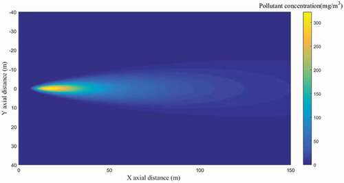
Table 2. Simulation parameters.

Parameters	Value
Area	150 × 80 m
Pollution source location	(0 m, 20 m)
Gas release speed	1–10 g/m
Height of the pollution source	1 m
Wind speed	0.5–1 m/s

According to the analysis of the MATLAB simulation results, the gas concentration distribution of the Gaussian pollutant diffusion model in the entire field source is symmetrical about y = 0, the pollution source diffused downwind toward the x axis, the gas concentration value gradually decreased, and the diffusion distance was long. The pollutant concentration in the upwind direction of the pollution source was very small and close to zero. The pollutant concentration was densely distributed in the vertical x-axis direction, and the diffusion distance was short; thus it was a stable, smooth, and ideal gas diffusion model.

Gas diffusion simulation in a complex environment was an irregular turbulent motion process. Turbulence is an extremely complex and non-linear fluid motion. In turbulent motion, various physical parameters (pressure, temperature, speed, etc.) change constantly with time and space. The GAMBIT software is a software package designed to integrate computational mechanics and physical models into computational fluid dynamics (CFD) models (Wang 2018). In this study, it was used to establish a model of the UAV flight environment in a three-dimensional space of 100 × 50 × 20 m³. The air pollution source was set in a three-dimensional space at the location (20 m, 25 m), where and the height was 10 m, the air pollution source release speed was 1–10 g/s, the polluted gas mass fraction (C) was 1, and the wind inlet velocity was 0.5–1.0 m/s. The ambient pressure was the standard atmospheric pressure, (Pa), the temperature was 300 K, and there were pressure outlets all around. the space. Current turbulence models for the diffusion of atmospheric pollutants mainly include the k–ε, k–ω, SSG and SST. This study used the k–ε model based on the eddy current viscosity theory, which not only has wide applicability but also high calculation accuracy. after the parameters obtained from the FLUENT calculation are listed in Table 3. The results of the simulation calculation with z = 12 m are intercepted, as shown in Figure 7.

Figure 7. Pollutant diffusion simulation in a complex environment.

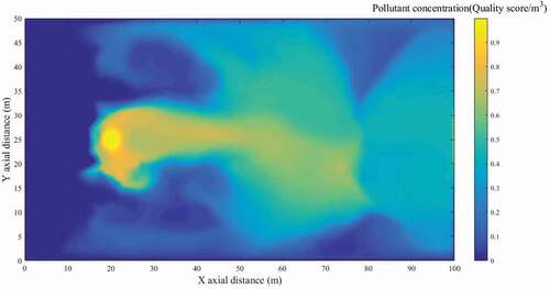
Table 3. Simulation parameters.

Parameters	Value
Area	100 × 50 × 20 m
Pollution source location	(20 m, 25 m, 10 m)
Gas release speed	1–10 g/m
Ambient pressure	$1.01\times {10}^5$ Pa
Wind speed	0.5–1 m/s
Temperature	300 K
Turbulence model	k-ε model

Performance metrics

Two metrics, the distance ratio and success rate, are generally used to evaluate the performance of FCT algorithms.

The distance ratio (d₀) is the flying distance (d_t) of the UAV divided by the length (d_u) of the shortest path connecting the starting point and source of pollution. The distance ratio was used here because it indirectly reflected the time spent in the experiment. To a certain extent, the distance ratio in this study represents the traceability efficiency of the algorithm, which can be expressed mathematically by Equation (3)(3) ${\mathrm{d}}_0=\frac{d_t}{d_u}$(3) .

(3) ${\mathrm{d}}_0=\frac{d_t}{d_u}$(3)

The lower the d₀, the better the performance of the algorithm and the higher the efficiency. The algorithm achieved the best performance when d₀ was 1.

The second metric, the success rate (Sr), is the ratio of the number of successes (or the frequency of successful traceability with a specific time or iteration time) to the total number of experiments.

Traceability algorithm for a single UAV

To compare and explain, in this chapter, the representative bio-inspired ZigZag and the FCT algorithms in bionics are selected, and changes in the two parameters of wind speed and source intensity are compared and analyzed.

Experimental evaluation

The FCT and the ZigZag algorithm were simulated under an ideal environment (Gaussian pollutant diffusion model) and complex conditions (time-varying complex gas diffusion model simulated by FLUENT software), respectively, and then these data were used to calculate the model performance. Figure 8 shows the typical trajectories of the two algorithms in the Gaussian concentration field. Figure 11 shows the typical trajectories of the two algorithms in a complex concentration field. Figures 9, 10, 12, and 13 show the results of randomly selecting the starting point position of both algorithms in each different environment ten times. The box plots in the lower panel of Figures 9, 10, 12, and 13 show the distance ratio, which can vary significantly under different circumstances, while the Sr of each set of numerical simulations is represented by a bar graph at the top of the figure.

Figure 8. Trajectories of the FCT algorithm(left) and the ZigZag algorithm(right) obtained in the Gaussian concentration field.

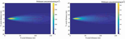
Figure 9. Tracing results of the FCT algorithm(left) and the ZigZag algorithm(right) under Gaussian environmental conditions with different wind speed.

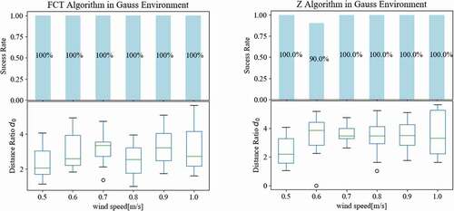
Figure 10. Tracing results of the FCT algorithm(left) and the ZigZag algorithm(right) under Gaussian environmental conditions with different gas release speeds.

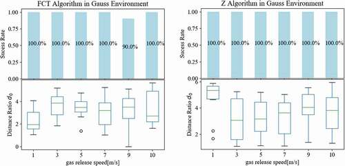
Figure 11. Trajectories of the FCT algorithm(left) and the ZigZag algorithm(right) obtained in the Gaussian concentration field.

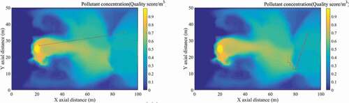
Figure 12. Tracing results of the FCT algorithm (left) and the ZigZag algorithm (right) in a complex environment with different wind speeds.

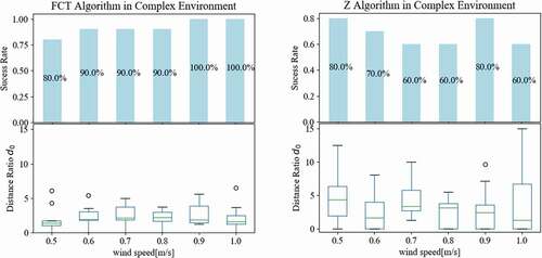
Figure 13. Tracing results of the FCT algorithm and the ZigZag algorithm in a complex environment with different gas release speed.

Gaussian concentration field

Figure 8 shows the trajectories of the two algorithms in the Gaussian concentration field. The figure on the left shows the pollution source tracking path using the FCT algorithm. The figure on the right shows the use of ZigZag algorithm to track the paths of pollution sources.

Figure 9 shows the influence of the wind speed on the simulation results of the two algorithms, wherein the Srs of the FCT and ZigZag algorithms are both relatively high in an ideal environment. In this round of experiments, when the wind speed was set to 0.6 m/s, the Sr of the ZigZag algorithm was 90%, indicating that the wind speed has a certain influence on the ZigZag algorithm. However, the Sr of the FCT algorithm was 100% under different wind speed conditions, which indicates that the Sr of the FCT algorithm is optimal over the ZigZag algorithm. In contrast, the distance ratio of the two algorithms was similar; however, the distance ratio of the FCT algorithm was slightly better than that of the ZigZag algorithm overall except for several groups of data. This conclusion is reached through the median distance ratio between the two algorithms.

Figure 10 shows the influence of the gas release speed on the simulation results of the two algorithms. In an ideal environment, the FCT and ZigZag algorithms were not significantly affected by the source strength. In this round of experiments, when the release intensity Q of the pollution sources was set as 1 m/s, the Sr of ZigZag algorithm was 100%, owing to the strong searching ability of ZigZag for smoke plumes. However, some experiments using the FCT algorithm failed to find the plume; therefore, its Sr was only 90%. The FCT algorithm had a higher traceability efficiency and Sr in the plume; however, its ability to find the plume was not as good as that of the ZigZag algorithm.

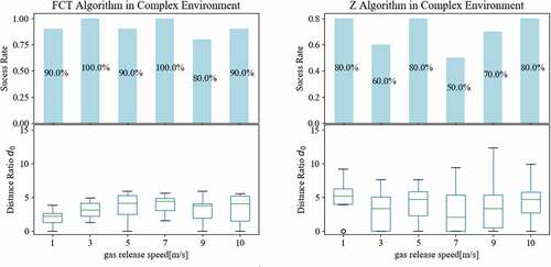
Complex concentration field

Figure 11 shows the trajectories of the two algorithms in a complex concentration field. The figure on the left shows the use of the FCT algorithm to track the pollution source path, while the figure on the right shows the ZigZag algorithm used to track the pollution source path.

Figure 12 shows the simulation results of the FCT and ZigZag algorithm for the wind speed change in a complex environment. In this round of experiments, the release rate of the pollution source was set to a constant value of 2 m/s. Six different wind speed conditions were set: 0.5, 0.6, 0.7, 0.8, 0.9, and 1.0 m/s. In terms of the Sr, in complex environments, FCT algorithm had obvious advantages over the ZigZag algorithm, as it had more delicate and flexible search ability for pollution sources, while the Sr of ZigZag algorithm was not accurate, especially in the experimental group where the wind speed was 0.7, 0.8 m/s, the Sr of traceability was only 60%. Conversely, the distance ratio of the FCT algorithm was below 6, and the median was approximately 2. The distance of the ZigZag algorithm, however, was 15 compared with the highest value of d₀, and the median was approximately 4, so the tracing efficiency was low.

Figure 13 shows the simulation results of the FCT and ZigZag algorithm for the gas release speed change in a complex environment. In this round of experiments, the wind speed was set to a constant 0.5 m/s, and six different conditions were set for the release rate of pollution sources: 1, 3, 5, 7, 9 and 10 m/s. In terms of Sr, the FCT algorithm had obvious advantages in a complex environment. The Sr of the ZigZag algorithm was higher than that of the wind speed change, but still not optimal. In the experimental group, where the release speed of the pollution source was set to 7 m/s, the tracing Sr was only 50%. Contrarily, the distance ratio of the FCT algorithm was below 6 and the distance of the ZigZag algorithm was 12, compared to the highest value of d₀, and the median was approximately 4, indicating low tracing efficiency.

Result and discussion

In this chapter, the above simulation comparison of the FCT algorithm and ZigZag algorithm under time-varying environments (Gaussian pollutant diffusion model) and complex situations (time-varying complex gas diffusion model simulated by FLUENT software) assessed the advantages and disadvantages of the two algorithms. In an ideal environment (Gaussian pollutant diffusion model), the Sr of the FCT algorithm and ZigZag algorithms were very high, and the tracing efficiency was no less than that under the ideal environment (Gaussian pollutant diffusion model), regardless of wind speed or release intensity of pollution sources. However, in the complex case (the time-varying complex gas distribution model simulated by FLUENT software), although Sr could not reach 100%, the FCT algorithm could search the pollution area more delicately and flexibly according to our preset rules with a better traceability efficiency, while ZigZag algorithm could not adapt its the relatively more simple search logic to compare with the FCT algorithm.

Traceability algorithm for multiple UAVs

The last chapter introduced a single UAV traceability algorithm based on fuzzy control and a set of traceability simulation experiments in an environment based on FLUENT and MATLAB. In view of the shortcomings of a single UAV in the traceability task, this section further reports the improvement of the traceability algorithm of fuzzy control and proposes a traceability algorithm that can be applied for multiple UAVs.

Strategy

Multiple UAVs can be viewed as a population, composed of three roles: master, slave, and reconnaissance UAV, as shown in Figure 14.

Figure 14. Schematic diagram of UAV population.

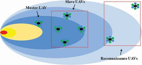
(1) The location of the master was the location where the highest concentration was found in the current traceability task.

(2) The slave plays represent the local search ability of the refined population in the area surrounding the master.

(3) A reconnaissance UAV is used to conduct a random search and improve the global optimal ability of the population search.

(4) The basic principle of master location update: Each location update in the traceability task is updated according to the fuzzy control-traceability algorithm of a single UAV.

(5) The basic principle of the slave location update: Each position update in the traceability task is based on the master position update rules, and the position and concentration difference of the master are comprehensively quantified as an index (master information), which can be compared with the density information of other directions horizontally, as a modification rule of the fuzzy control traceability rule of a single UAV.

(6) The basic principle of reconnaissance UAV location update: The position update is based on a random walk strategy, wherein the move length of each update is relatively large and the angle of rotation is also a random value.

(7) The role of the population is also updated every time its position is updated. The master has the highest concentration after the update each time, and the reconnaissance UAV has the lowest gas concentration.

(8) While there is only one master, the number of slave and reconnaissance UAVs can be reallocated according to the corresponding rules.

Slave location update strategy

Each location update in the traceability task was based on the master location update rules, which comprehensively quantified the master location and concentration difference into an index (master information), denoted as massage_M. The fuzzy language description of the gas concentration measured by the gas sensor mounted on the slave was the same as that of the master. After the slave was updated according to the fuzzy control-traceability algorithm of a single UAV, the master information was used as an additional indicator for the output of the slave. The angle and step information are corrected in accordance with certain rules so that each slave could process its own gas concentration and environmental information and then synthesized the relevant information from the master to perform an efficient traceability search. The update strategy of a slaver location is shown in Figure 15.

The correction rule is as follows: The highest gas concentration measured by the master should be compared with the highest gas concentration measured by the slave.

(1) If the concentration level has the same intensity, the slave is not affected by the master information, and the slave position is updated according to the move length and angle calculated by the fuzzy control traceability algorithm of a previous single UAV.

(2) If the concentration level of the slave is greater than that of the master, the slave will be regarded as the new master and will not be affected by the original master information, and the location is updated according to the update strategy of the previous master location.

(3) If the concentration value of the slave is less than that of the master, the update strategy must be corrected according to the position of the master; that is, direction A1 of the next update position of the slave is replaced with the synthesis direction of the directions A0 and A1 of the master relative to the position of the slave. The move length of the slave update position remains constant.

Reconnaissance UAV location update strategy

The position update of a reconnaissance UAV was based on a random-walk strategy to improve the global optimal ability of the population search. In particular, when the master and slave groups fell into a local optimum, the global optimization capability of the reconnaissance UAV could be well reflected; the move length of each position update of the reconnaissance UAV was relatively large, and the angle of rotation was also a random value, as shown in Equation (4)(4) $Angle=\alpha ,ST=r{d}_{max}$(4) ,

(4) $Angle=\alpha ,ST=r{d}_{max}$(4)

where $\alpha$ is a random direction, r is a random constant generated by a normal distribution with an average value of zero and a standard deviation of one, and d_max is the maximum move length in the master location update strategy.

Dynamic population allocation strategy

After updating the positions of all individuals in the population each time, make a comprehensive judgment (i.e., the diversity of the population) should be made according to the environment of the individual and the number of each role to determine whether an update was warranted in implementing the characteristics of the dynamic populations of the algorithm. In this study, the diversity of the population was measured using the Shannon-Wienner diversity index, as shown in Equation 5(5) $D=1-\sum _{i=1}^S\frac{N_i}{N}\mathrm{I}\mathrm{n}\frac{N_i}{N}\hspace{0.17em}i=(1,\hspace{0.17em}2,\hspace{0.17em}\dots ,\hspace{0.17em}S)$(5) ,

(5) $D=1-\sum _{i=1}^S\frac{N_i}{N}\mathrm{I}\mathrm{n}\frac{N_i}{N}\hspace{0.17em}i=(1,\hspace{0.17em}2,\hspace{0.17em}\dots ,\hspace{0.17em}S)$(5)

where S is the number of roles in the group, N is the number of individuals in the entire group, N_i is the number of individuals in i, and D is the Shannon-Wienner index quantitative index of the population diversity. The larger the value of D, the stronger the population diversity. The threshold range of the population diversity should be set to [D₀, D₁].

The population update strategy is as follows:

(1) If there is only one master, the number of slaves and reconnaissance UAVs can be redistributed according to their corresponding rules.

(2) The master has the highest concentration after the population location is updated.

(3) The reconnaissance UAV has the lowest gas concentration each time, and the concentration of the population individuals should be calculated after the position is updated to Concentration(i), i = 1, …, N. The individuals are sorted according to the concentration value in order of increasing size, and the Q individuals with the smallest concentration are selected as the reconnaissance UAVs after sorting. The size of Q is the number of reconnaissance UAV depending on the total number of populations.

(4) The diversity of the population is maintained between D₀ and D₁.

(5) A diversity value below the threshold D₀ indicated that the diversity of the population is poor. The number of reconnaissance UAVs should be increased and the number of slaves should be reduced in response to improve the global optimization ability of the population search, which can be generated according to a uniform distribution. A random number between [0% and 20%] can be generated according to a uniform distribution. This random number is multiplied by the total population S to obtain the value of the increased number of reconnaissance UAVs.

(6) A diversity value greater than the threshold value D₁, indicated that the diversity of the population is high. Therefore, the number of slaves can be increased and the number of reconnaissance UAV can be reduced, to improve the local optimization performance of the population. A random number between [0% and 20%], should be generated according to the uniform distribution. This random number is multiplied by the total population S, and the value obtained is reduced the number of reconnaissance UAVs.

Experimental evaluation

This section mainly discusses changes in the total number of populations in the traceability algorithm, the atmospheric wind speed of the background concentration field and the source intensity of atmospheric pollutants, as a means to explore the influence of the changes in these three factors on the algorithm described in this chapter. The termination conditions are as follows: concentration_max = 300, iteration_max = 1000, threshold range of population diversity [0.2, 0.8], and the total number of population individuals N = 3, 5, 7, 9.

Gaussian concentration field

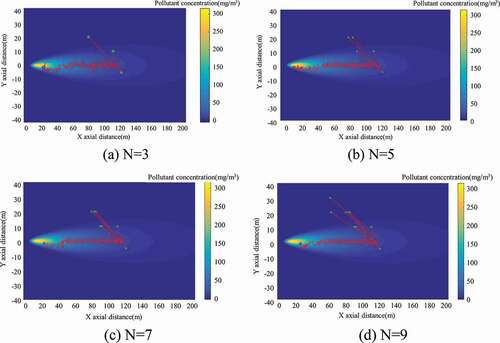
Sixteen different experiments were set up under steady-state conditions, and the two algorithms were run ten times each in different environments. The first six groups were used to keep the total population of the algorithm N = 3 unchanged, the source intensity of air pollutants was set to a constant 2 g/s in the Gaussian plume diffusion model, and change in wind speed u was set to 0.5, 0.6, 0.7, 0.8, 0.9 and 1.0 m/s respectively; in the middle six groups, the total population N = 3 of the algorithm was constant, the wind speed u was set to a constant 0.5 m/s, and the release intensity of air pollutants was changed to 1, 3, 5, 7, 9, and 10 g/s, respectively; the release intensity of air pollutants in the last four groups of experiments was 2 g/s, the wind speed u was a constant 0.5 m/s, and the total population of the algorithm was N = 3, 5, 7 and 9 respectively.

Figures 16 (a) and (b) show the resulting simulation statistics of the multi-UAV traceability algorithm based on fuzzy control under steady-state conditions under varying the wind speeds and source intensities. In this round of experiments, the Sr of the multi-UAV traceability algorithm based on fuzzy control was 100%, indicating that the Sr of the algorithm under steady-state conditions was insensitive to changes in environmental factors. However, the single UAV traceability algorithm based on fuzzy control failed to find the smoke plume in the experiment where source strength was altered, so the Sr of the algorithm in this chapter was better under steady-state conditions. In terms of distance ratio, the algorithm in this chapter, owing to the position update strategy of the random walk of the reconnaissance UAV role, enhanced the global search capability of UAV populations, as well as the total distance of the population search to a certain extent. Therefore, the algorithm in this chapter was not prominent in the distance ratio, but the median of the distance ratio was basically maintained within 4, which had little impact on the overall traceability efficiency. Figure 16(c) shows the resulting simulation statistics of the multi-UAV traceability algorithm based on fuzzy control with varying total numbers of traceable UAV populations under steady-state conditions. Changing the total number of populations had no effect on the Sr of traceability; all were 100%, but the median of the distance ratio indicated that as the total population increased, the distance ratio decreased significantly, and thus the traceability efficiency also increased. Figure 17 shows a simulation diagram of the multi-UAV traceability algorithm based on fuzzy control under steady-state conditions with N = 3, 5, 7, and 9.

Figure 15. Schematic diagram of a slave location update strategy.

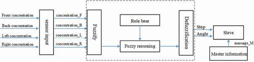
Figure 16. Analysis of simulation results under steady-state conditions. (a) Wind speed, (b) Source intensity, (c) Total population.

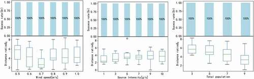
Figure 17. Schematic diagram of traceability algorithm simulation.

Complex concentration field

A set of 16 experiments were set up under complex turbulent conditions. The first six groups were chosen to keep the total population of the algorithm N = 3 unchanged, the release rate of air pollutants in FLUENT was set to 2 m/s,, and the wind speed u was set to 0.5, 0.6, 0.7, 0.8, 0.9 and 1.0 m/s, respectively; the middle six groups also retained the N = 3 conditions, but the wind speed u of 0.5 m/s was constant, while the release intensity of air pollutants were set to 1, 3, 5, 7, 9, 10 m/s; the release intensity of atmospheric pollutants in the last four groups of experiments was 2 m/s and the atmospheric wind speed u was 0.5 m/s, only the algorithm was changed The total number of populations N = 3, 5, 7, 9.

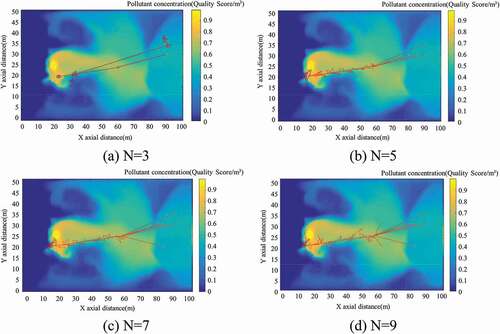
Figures 18 (a) and (b) show the simulation result statistics of the multi-UAV traceability algorithm based on fuzzy control, factory in changing wind speed and source intensity under complex turbulent conditions. Compared with Figures 12 and 13, the proposed algorithm was significantly more accurate than both the single UAV traceability algorithm based on fuzzy control and the ZigZag algorithm. Figure 18(c) shows the simulation statistics of the multi-UAV traceability algorithm based on fuzzy control factoring in changes in the total number of traceable UAV populations under complex turbulent conditions. The schematic diagram shows that the total number of populations affected the improvement of traceability Sr, and the median the distance ratio indicated that, as the total number of population’s increased, the distance ratio decreased significantly, which implied that as the total population increases, the traceability efficiency also increased. Figure 19 shows a simulation diagram of the algorithm under complex turbulent conditions with N = 3, 5, 7, and 9.

Figure 18. Analysis of simulation results under complex turbulent flow conditions. (a)Wind speed, (b) Source intensity, (c) Total population.

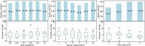
Figure 19. Schematic diagram of traceability algorithm simulation where N = 3 (a), 5 (b),7 (c), and 9 (d).

Result and discussion

The single-UAV traceability algorithm based on fuzzy control, combined with the characteristics of each role in the population, resulted in a multi-UAV traceability algorithm based on fuzzy control, which we propose here. The position update and population allocation strategies of the slave and reconnaissance UAVs in the algorithm role are introduced in detail, and the implementation steps of the algorithm are sorted out. Finally, the simulation experiment using multiple concentration fields provided in Chapter 2, proves the superior performance of the proposed multi-UAV traceability algorithm based on fuzzy control in terms of search efficiency and Sr.

Conclusion

Considering the complexity and multifaceted nature of air pollutants, this study proposed a fuzzy control method for tracing air pollution using UAVs. The algorithm combined the characteristics of UAVs and rules of fuzzy control to imitate the thinking of the human brain to identify, judge, and process gas concentrations, which could effectively solve the problem of traceability of atmospheric pollutants in complex environments. To prove the excellent performance of the FCT algorithm, we compared the FCT algorithm with the ZigZag algorithm. In this study, multiple sets of experiments were conducted, and the results verified that the FCT algorithm had good applicability and robustness in the traceability of pollutants.

Fuzzy control logic was applied to the field of air pollutant traceability of UAVs, and a single UAV traceability algorithm based on fuzzy control was proposed, in which multiple traceability subjects were introduced to optimize the FCT algorithm, and then a multi-UAV traceability algorithm based on fuzzy control was proposed. The algorithm divided the UAV group into three roles, dynamically allocated the number of population roles according to the diversity of the population, and verified its superior performance through simulation experiments, thereby solving the shortcomings of a single UAV as the main body of traceability.

Finally, in future, endeavors to improve the efficiency of the FCT algorithm, wind speed direction information should be added to the slate of input variables of the fuzzy controller, and formulate corresponding fuzzy control rules.

Disclosure statement

No potential conflict of interest was reported by the author(s).

Data availability statement

The data that support the findings of this study are available from the corresponding author, Tao Ding, upon reasonable request.

Additional information

Funding

This study was supported by the Natural Science Foundation of Zhejiang Province [LGF20E080014].

Notes on contributors

Xinyan Jiang

Xinyan Jiang is a graduate student affiliated with the College of Quality and Safety Engineering, China Jiliang University, Hangzhou, China.

Tao Ding

Tao Ding is an associate professor affiliated with the College of Quality and Safety Engineering, China Jiliang University, Hangzhou, China.

Yuting He

Yuting He is a graduate student affiliated with the College of Quality and Safety Engineering, China Jiliang University, Hangzhou, China.

Xuelin Cui

Xuelin Cui is a graduate student affiliated with the College of Quality and Safety Engineering, China Jiliang University, Hangzhou, China.

Zhenguo Liu

Zhenguo Liu is a graduate student affiliated with the College of Quality and Safety Engineering, China Jiliang University, Hangzhou, China.

Zhenming Zhang

Zhenming Zhang is a graduate student affiliated with the College of Quality and Safety Engineering, China Jiliang University, Hangzhou, China

References

- Cheng, D., J. E. Feng, and H. Lv. 2012. Solving fuzzy relational equations via semitensor product. Fuzzy Syst. IEEE Trans 20 (2):390–96. doi:10.1109/TFUZZ.2011.2174243.
- Demetriou, M. A., T. Egorova, and N. A. Gatsonis. 2016. Estimation of a gaseous release into the atmosphere using a formation of UAVs. IFAC-PapersOnLine 49 (18):110–15. doi:10.1016/j.ifacol.2016.10.148.
- Fu, Z., Y. Chen, and Y. Ding, D. He. 2019. Pollution source localization based on multi-UAV cooperative communication. IEEE Access, 29304–12.
- Fu, J., L. Y. Shen, and R. R. Liu. 2021. An indoor odor source locating method for multi-robot active olfaction based on improved AEO. Chin. J. Sens. Actuators 34:1406–11.
- Ge, A. D., Y. Z. Wang, A. R. Wei, and H. B. Liu. 2013. Control design for multi-variable fuzzy systems with application to parallel hybrid electric vehicles. Control Theory Appl 30 (8):998–1004.
- Gideon, K., R. A. Russell. 2008. Robot odor localization: A taxonomy and survey. Int. J. Rob. Res 27 (8):869–94. doi:10.1177/0278364908095118.
- Gu, J., S. Tao, Q. Wang, X. Du, and M. Guizani. 2018. Multiple moving targets surveillance based on a cooperative network for multi-UAV. IEEE Commun. Mag 56 (4):82–89. doi:10.1109/MCOM.2018.1700422.
- Hu, C. 2021. Attitude stability control of UAV gyroscope based on neutral statistics for smart cities. Int. J. Syst. Assur. Eng. Manag 13:281–290. https://doi.org/10.1007/s13198-021-01391-6.
- Ishida, H., K. Suetsugu, T. Nakamoto, and T. Moriizumi. 1994. Study of autonomous mobile sensing system for localization of odor source using gas sensors and anemometric sensors. Sensors and Actuators A: Physical. 45 (2):153–57. doi:10.1016/0924-4247(94)00829-9.
- Jatmiko, W., K. Sekiyama, and T. Fukuda 2006. A PSO-based mobile sensor network for odor source localization in dynamic environment: Theory, simulation and measurement. IEEE Congress on Evolutionary Computation, 1036–43. Vancouver, BC, Canada: IEEE.
- Kowadlo, G., and R. A. Russell. 2009. Improving the robustness of nave physics airflow mapping, using Bayesian reasoning on a multiple hypothesis tree. Rob. Auton. Syst 57:723–37. doi:10.1016/j.robot.2008.10.019.
- Li, H., and Y. Wang. 2013. A matrix approach to latticized linear programming with fuzzy-relation inequality constraints. IEEE Trans. Fuzzy Syst 21 (4):781–88. doi:10.1109/TFUZZ.2012.2232932.
- Li, Y., K. Li, and S. Tong. 2020. Adaptive neural network finite-time control for multi-input and multi-output nonlinear systems with positive powers of odd rational numbers. IEEE Trans. Neural Networks Learn. Syst 31 (7):2532–43.
- Li, Y., T. Yang, and S. Tong. 2020. Adaptive neural networks finite-time optimal control for a class of nonlinear systems. IEEE Trans. Neural Networks Learn. Syst 31 (11):4451–60.
- Lochmatter, T. J. E. 2010. Bio-inspired and probabilistic algorithms for distributed odor source localization using mobile robots. epfl. 135. doi:10.5075/epfl-thesis-4628.
- Longinus, N. K., R. T. John, and A. M. Olatunde, Adesuyi, A. A., & Jolaoso, A. O. 2016. Ambient air quality monitoring in metropolitan City of Lagos, Nigeria. J. Appl. Sci. Environ. Manag 20 (1):178–85. doi:10.4314/jasem.v20i1.21.
- Lu, G. D., X. J. Zhang, and J. H. Li. 2010. Robot bionic active olfaction strategy based on wandering albatross behavior. J. Mach. Des 27 (11):43–47.
- Meng, Q. H., and F. Li. 2006. Review of active olfaction. Robot 28 (1):89–96.
- Park, M., and H. Oh. 2020. Cooperative information-driven source search and estimation for multiple agents. Inf. Fusion 54:72–84. doi:10.1016/j.inffus.2019.07.007.
- Qiu, S., B. Chen, R. Wang, Z. Zhu, Y. Wang, and X. Qiu. 2017. Estimating contaminant source in chemical industry park using UAV-based monitoring platform, artificial neural network and atmospheric dispersion simulation. RSC Adv 7 (63):39726–38. doi:10.1039/C7RA05637K.
- Russell, R. A. 1999. Ant trails - an example for robots to follow? Proceedings of the Proceedings 1999 IEEE International Conference on Robotics and Automation, vol. 4, , 2698–703. Detroit, Michigan,USA.
- Russell, R. A., A. Bab-Hadiashar, R. L. Shepherd, and G. G. Wallace. 2003. A comparison of reactive robot chemotaxis algorithms. Rob. Auton. Syst 45 (2):83–97. doi:10.1016/S0921-8890(03)00120-9.
- Russell, R. A. 2004a. Locating underground chemical sources by tracking chemical gradients in 3 dimensions. Proceedings of the IEEE/RSJ International Conference on Intelligent Robots & Systems, vol. 1, 325–30. Sendai, Japan.
- Russell, R. A. 2004b. Chemical source location and the robomole project. Aust. Rob. Autom. Assoc. 1–6.
- Vergassola, M., E. Villermaux, and B. I. J. N. Shraiman. 2007. ‘Infotaxis’ as a strategy for searching without gradients. Nature 445 (7126):406–09. doi:10.1038/nature05464.
- Wang, Y. X. 2018. Simulated calculation of flue gas mixing flow field. Shandong Chem. Ind 47 (15). 177-179. doi:10.19319/j.cnki.issn.1008-021x.2018.15.073.
- White, B. A., A. Tsourdos, I. Ashokaraj, S. Subchan, and R. Zbikowski. 2008. Contaminant cloud boundary monitoring using network of UAV sensors. IEEE Sens. J 8 (10):1681–92. doi:10.1109/JSEN.2008.2004298.
- Zhang, X. J., M. L. Zhang, Q. H. Meng, and J. Li. 2008. A gas/odor source localization strategy for mobile robot based on animal predatory behavior. Robot 30 (3):268–72.