Optimization of multi-frequency electromagnetic surveying for investigating waste characteristics in an open dumpsite

ABSTRACT

Multi-frequency electromagnetic (EM) surveying is a type of frequency-domain electromagnetic (FDEM) survey, a new geophysical exploration approach used as a scanning tool to investigate waste characteristics within a final disposal site before electrical resistivity tomography (ERT) surveying. EM surveys provide information about shallow subsurface conditions; however, to date, no studies on waste bodies or waste characteristics in open dumpsites have assessed the optimal frequency for use in multi-frequency EM surveys. This research aims to determine the optimal frequency set for multi-frequency EM surveying for initial waste quality assessment in open dumpsites. These initial waste quality data are critical to assess the feasibility of open dump mining projects. First, a multi-frequency EM survey was performed in this study, which was measured at the exact electrode positions of the three ERT profiles. This FDEM survey used 15 frequencies ranging from 1,000–⁠15,000 Hz, which were grouped into frequency sets for inversion modeling of the electrical conductivity. Second, an ERT survey was carried out along all three profiles, each of which was around 144 m long. Subsequently, synthetic electrical resistivity data were generated by processing the electrical conductivity model. Data from each frequency set were then generated at the same depth, with interpolation techniques used to analyze the linear correlation between synthetic electrical resistivity and real electrical resistivity data and compare the Pearson’s correlation coefficient (R) values to determine the optimum frequency set for FDEM surveys in the open dumpsite. The results showed that the E4 frequency set, consisting of 5,000, 11,000, and 15,000 Hz values, typically had the highest positive correlations (R = 0.74–0.91) across all profiles and provided waste characteristics information close to the true conditions. Thus, these frequencies represent the optimal set for multi-frequency EM surveys for the primary assessment of waste characteristics in open dumpsites.

Implications: Open dump mining (ODM) is now applied as a sustainable approach to combat improper waste disposal and reduce municipal solid waste (MSW) in the open dumpsite. To implement ODM for producing RDF, business developers must know the amount and composition of waste that can be converted into RDF before mining. This study used multi-frequency EM surveys with frequencies of 5,000, 11,000, and 15,000 Hz. This multi-frequency method effectively determined the waste composition and identified potential excavation points in the open dumpsite prior to ODM. This method can mitigate the limitations of traditional surveying, due to its improved mobility, lower time consumption, and reduced labor needs.

Introduction

Open dumping (OD) is a prevalent waste disposal method in developing countries. In Thailand, open dumpsites can be found in all regions due to their low cost and ease of operation (Prechthai, Padmasri, and Visvanathan 2008; Sharma et al., 2018). However, this method is an improper waste management system whose problems include a lack of control over the type of waste being disposed of, an absence of soil cover over waste sites, and the possibility of open burning of some waste. Improper waste handling protocols will lead to an increased volume of mismanaged waste, causing severe pollution and environmental contamination problems (Chiemchaisri et al., 2008; Maheshi, Steven, and Karel 2015). Open dump mining (ODM) is now being applied as a sustainable approach to combat improper waste disposal and help to reduce municipal solid waste (MSW) in open dumpsites. The ODM process involves excavating waste in an open dumpsite and separating it for raw material extraction through waste to material conversion and refuse-derived fuel (RDF) for waste to energy conversion (Carius et al. 1999; Rosendal 2009; Maheshi, Steven, and Karel 2015; Sharma et al., 2019; Wangyao, Sutthasil, and Chiemchaisri 2021).

To implement ODM for RDF production, business developers must identify the amount and composition of waste that can be potentially converted to RDF before mining. The amount of waste can be determined through topographic surveys or unmanned aerial vehicle photogrammetry surveys (Bhatsada et al. 2020). However, a major problem in ODM operations is a lack of available information on the composition of partially degraded waste. Geophysical exploration methods are now widely applied in waste processing because they are noninvasive, less time-consuming in the field than other methods, and can successfully characterize waste. These factors result in lower costs and reduced environmental impacts compared to conventional surveys (i.e., direct waste sampling by excavation and gas flux measurement) (Rosquist et al. 2011; Maio et al. 2018; Boonsakul et al. 2021; Chungam et al. 2021).

Frequency-domain electromagnetic (FDEM) surveying is a common geophysical survey method, which is widely used in waste work in conjunction with the electrical resistivity tomography (ERT) survey method. The FDEM technique enables various preliminary studies of waste disposal areas, including inspecting groundwater contamination from leachate, inspecting the geological and structural characteristics of final disposal sites, mapping the boundaries of final disposal sites, and inspecting waste composition within landfill sites (Shemang et al., 2011; Osinowo, Falufosi, and Omiyale 2018; Kondracka et al. 2021; Deidda et al. 2022).

FDEM surveys work by generating a primary electromagnetic (EM) field (H_p) at different frequencies, which is passed through the ground surface. When the H_p field passes through a conductive object, it induces eddy currents around the object, thus producing a secondary electromagnetic field (H_s). Subsequently, both fields combine to induce a current in the receiver coil. This complex field is then decomposed into its real and imaginary components (i.e., in-phase and quadrature components, respectively) after subtraction of the principal magnetic field. The imaginary components are converted to apparent electrical conductivity (σ_a); this parameter is processed to determine the subsurface characteristics of the electrical conductivity (EC or σ) and depth of investigation (DOI) (McNeill 1980).

FDEM surveys to assess and investigate final waste disposal sites are commonly conducted using a single frequency and multi-coil orientations. Previous studies have used single-frequency surveys to characterize leachate plumes (Bichet, Grisey, and Aleya 2016), investigate landfill site structures (Fraga et al. 2019), map waste disposal areas (Soupios et al. 2007), and inspect groundwater contamination (Kaya, Özürlan, and Şengül 2007). However, previous surveys using a single frequency with multi-coil orientations have identified some limitations of using this method to examine the waste composition and physical characteristics of open dumpsites (Soupios and Ntarlagiannis 2017; Isunza Manrique et al. 2019). These limitations arose because the waste was heterogeneous, with high porosity and low density, resulting in reduced single-frequency waves traveling through the medium, thus making it impossible to interpret the significance of the modeled EC distribution. Although density does not exhibit a direct first-order relationship with electrical properties, the movement of electric currents to the surface of the ground is nonetheless influenced by density (Kaufmann 2014; Hunkeler et al. 2015).

Modern multi-frequency EM surveys are conducted using a single-coil orientation to counteract the issue of data ambiguity in single-frequency surveys. Kaufmann (2014) and Hunkeler et al. (2015) identified that using multiple frequencies for an FDEM survey is more effective than using single frequencies. Multi-frequency surveys allow improved subsurface wave transmission, reduce the limitations caused by high porosity media, and provide data from the EC layer that are more representative of real-world conditions. These advantages allow the volume and thickness of the waste layer to be more effectively characterized than with the use of a single frequency. Previously, multi-frequency surveys have been used in a variety of waste-related applications, such as assessing leachate movement in landfills (Ramalho, Dill, and Rocha 2012) and mapping final disposal sites (Osinowo, Falufosi, and Omiyale 2018). A previous study by Boonsakul et al. (2021) demonstrated that multi-frequency EM surveys are an efficient and reliable pre‑screening tool prior to ODM and can be used to estimate waste quality for RDF production. Past studies by Feng et al. (2017) have shown that ERT is a common and effective method to assess waste composition; however, this approach is labor-intensive, time-consuming, and costly. Consequently, the FDEM method is used to mitigate the limitations of ERT surveying, due to its improved mobility, lower time consumption, and reduced labor needs. In addition, although this method provides a shallower investigation than ERT surveying, FDEM surveys can be easily repeated after the waste has been excavated for RDF production. However, previous studies have not proposed an optimal frequency set for multi-frequency EM surveying to determine the waste composition in OD. This paper focuses on increasing the efficiency of multi-frequency EM surveys by finding the optimal frequency set for evaluating the composition and characteristics of waste in open dumpsites; accordingly, the objective of this study was to determine the optimal frequency set for multi-frequency EM surveys to be used as a scanning tool for preliminary waste quality assessment in OD before processing it into RDF.

Materials and methods

Site description

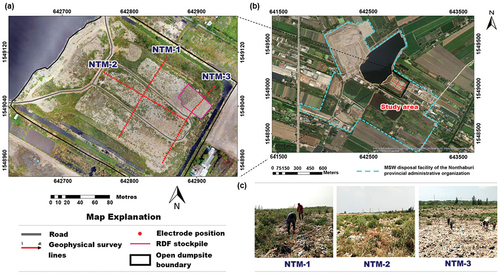
The study area is situated in the MSW disposal facility of the Nonthaburi provincial administrative organization (latitude 14.008417°N, longitude 100.322466°E), Khlong Khwang subdistrict, Sai Noi district, Nonthaburi province, Thailand. The study area covers approximately 35,000 m² and is located in a lowland area with an average height of 1–2 m above mean sea level, with slight elevation differences of 1–5 m (Figure 1). In 2018, this open dump contained a total waste volume of around 8,488,000 m³ and received approximately 1,300 tons of MSW per day (Xaypanya et al. 2018). The site’s waste consists of plastic material (e.g., polyethylene bags and other plastic), wood, textiles, soil-like material, and other material (Chiemchaisri, Charnnok, and Visvanathan 2010). This waste is around 7–12 years in age. In 2015, a private company reached an agreement with the Nonthaburi provincial administration organization to operate the ODM business and associated RDF power plant.

Figure 1. Site description; (a) Location and aerial image map of the study area showing ERT profile locations and EMP-400 profiler measurement points, (b) Map of MSW disposal facility of the Nonthaburi provincial administrative organization, Khlong Khwang subdistrict, Sai Noi district, Nonthaburi province, Thailand, and (c) Images showing surface conditions of each profile.

Data obtained from the Department of Mineral Resources of Thailand show that the geology of the study area is characterized by Quaternary sediments (flood plain clay on tidal flat clay on marine clay deposits). The climate of the study site is tropical. The average temperature is high throughout the year (24.2–32.5°C), with clear alternating rainy and dry seasons. The average relative humidity is 76.3%, and the average annual rainfall is approximately 1,795.5 mm.

Geophysical surveys

The geophysical methods used in this study consist of ERT and FDEM surveys, with data from the ERT survey used to generate a reference ER model. The reference ER model provided the true resistivity of the study site. This reference ER model was then directly compared with the EC model derived from the FDEM survey and the synthetic ER models obtained from inversion modeling of the EC data (Cavalcante Fraga et al. 2019). Obtaining comparable data using ER and synthetic ER is conducive to determining the FDEM survey’s optimal frequency in OD.

In this study, three geophysical survey profiles were acquired (NTM-1, NTM-2, and NTM-3 profiles), where the abbreviation NTM is used in the name of each profile, which stands for Nonthaburi dumpsite measurement. Each profile, 144 m long, was carried out during the fieldwork (Figure 1). The geophysical profiles are divided into two groups: (1) profiles NTM-1 and NTM-3, running northeast–southwest, and (2) profile NTM-2, running southeast–northwest. The survey was conducted from September to October 2020, at the end of the rainy season.

Data acquisition: ERT

The ERT survey was conducted by injecting direct current (I) through steel electrodes, creating a potential difference (∆V) between the electrodes. The potential difference was measured between different electrode pairs and the apparent resistivity (ρ_a) was then calculated (Eq. 1)(1) ${\rho }_a=K\frac{\mathrm{\Delta }V}{I}$(1) according to Ohm’s law (Milsom 2003). Therefore, ρ_a was calculated as follows:

(1) ${\rho }_a=K\frac{\mathrm{\Delta }V}{I}$(1)

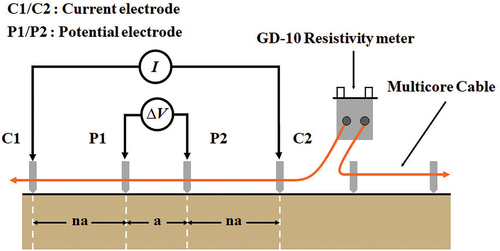
where ρ_a is the apparent electrical resistivity (Ω m), ΔV is the potential difference (mV), I is the electric current (A), and K is the geometrical factor (m). K is a numerical multiplier determined by the electrode configuration; the value of this geometric factor depends on the spacings between the current electrode (C₁ or C₂) and the potential electrode (P₁, P₂). The K value is used with the voltage-to-current ratio (R) to calculate ρ_a (Milsom 2003). The ERT survey was conducted using a GD-10 SUPREME 2D multi-electrode system (Geomative, China), and a Wenner–Schlumberger configuration (WS array) was used to collect data along all the survey lines. The WS array spacing between P1 and P2 electrodes was fixed in this array, as shown in Figure 2. The spacing between C₁ or C₂ and the potential electrode is proportional to the ratio n, which relates the distance between C₁ and P₁ to the distance between P₁ and P₂. Increasing n and the electrode spacing will increase the DOI. Furthermore, the DOI depends on the current density distribution, which is related to the length of the current dipole. The WS array can measure moderately sensitive/moderate resolution data both vertically and horizontally. This configuration is suitable for monitoring geological and environmental conditions in final disposal sites (Callegary, Ferré, and Groom 2007; Kondracka et al. 2021). In addition, the WS array configuration allows an exploration depth of 10 to 15% to be achieved, suitable for investigating the entire solid waste thickness and underlying basal sediment layers when the profile length exceeds 80 m (Barker 1989).

Figure 2. The electrode positions for the Wenner–Schlumberger configuration of the ERT survey.

In each of the three ERT survey profiles (NTM-1, NTM-2, and NTM-3), 48 electrodes were used, spaced 3 m apart, with all electrode coordinates measured using the real-time kinetic global navigation satellite system network (RTK-GNSS). RTK-GNSS is a satellite navigation technique that provides highly accurate positional data, with horizontal and vertical root mean squared error specifications of 8 mm ±0.5 ppm and 15 mm ±0.5 ppm, respectively (Bhatsada et al. 2020).

The ρ_a data were processed using RES2DINV 4.03.29 software (GEOTOMO SOFTWARE SDN BHD., Malaysia). The first processing step involves the removal of anomalous measurements (noise) from the field data, followed by the addition of the coordinates obtained from the RTK-GNSS. Next, the inversion is performed using the RES2DINV software; in this study, an iterative Jacobian matrix–constrained least-squares inversion approach was used to generate the actual ER model for the open dumpsite. The model processing can accurately estimate the DOI to create an ERT model that reflects the true configuration of the study area (Loke 2000). The resulting models were based on 800–810 points for all profiles (i.e., NTM-1, NTM-2, and NTM-3). In addition, the model provides root mean squared error (RMSE) values that show the percentage differences between the measured and calculated values of ρ_a in the fifth iteration of the ER model.

Data acquisition: FDEM

FDEM surveys are applied to investigate material and subsurface characteristics through different EC properties. The survey is performed by using the transmitter coil (T_x) to generate a primary electromagnetic field (H_p) from different frequencies of alternating current electricity. The T_x coil then releases the H_p field, which flows through the ground surface and air around the source. The H_p field induces a current around the conductor, generating an eddy current in the conductor. This eddy current produces a secondary electromagnetic field (H_s) that radiates outward. The H_s field interferes with the H_p field at any point on the surface and creates a net field, which is measured by the receiver coil (R_x). The net field is composed of in-phase field (I) and quadrature field (Q) components. The quadrature field is directly related to the EC of the ground surface and the conductivity anomaly (McNeill 1980). Accordingly, σ_a can be calculated as follows:

(2) ${\sigma }_a=\frac{4}{\omega s^2{\mu }_0}{\left(\frac{H_s}{H_p}\right)}_Q$(2)

where σ_a is the apparent electrical conductivity (mS/m), ω is the angular operating frequency (Hz) (ω = 2πf; f is the EM wave frequency), s is the inter-coil spacing (m) (profiler EMP-400 has a fixed coil spacing about 1.291 m), and μ₀ is the permeability of free space (4π × 10⁻⁷ H/m). The skin depth (δ) is the depth at which the transmitted magnetic field strength has decayed to an exponential level (i.e., e⁻¹ or 37%) of its initial magnitude at a reference point. In FDEM surveys, the effective δ varies inversely with the material’s resistivity and frequency (f): if δ increases, then the material’s frequency and resistivity decrease (Callegary, Ferré, and Groom 2007). The δ is defined by the expression:

(3) $\delta =\sqrt{\frac{2}{\sigma \mu \omega }}$(3)

This study measured the FDEM sounding at the electrode positions of ERT survey lines using a multi-frequency EM conductivity meter profiler (profiler EMP-400; Geophysical Survey Systems Inc., USA). The FDEM measurements were conducted along the same three profiles as the ERT survey (NTM-1, NTM-2, and NTM-3), as shown in Figure 1. Each profile consisted of 48 signaling points, and the EMP-400 profiler emitted an electric field at each signaling point at a height (h) of 0.4 m above the ground, producing an effective δ value of around 6–7 m. The optimum frequency survey applied 15 frequencies ranging from 1,000 to 15,000 Hz and used horizontal coplanar coils (HCP) or vertical magnetic dipole (VMD) coils with a constant coil spacing of 1.291 m. HCP coils are suitable for data detection in waste disposal sites and have greater sensitivity in deeper layers than vertical coplanar coils (VCP) (Callegary, Ferré, and Groom 2007; Piero Deidda et al. 2022).

Processing of σ_a obtained from the FDEM survey was conducted by inversion using EM4Soil-MF software (REFLEXOS Uni.P., Portugal). This software converts the σ_a data into a 2D EC model displaying the true EC that can be used to estimate the number of layers and the DOI. In addition, the EC data were used in this study for inverse processing to create a synthetic ER model.

This study used σ_a data from FDEM surveys with 15 different frequencies to group the frequency ranges using the random data method. Each frequency set comprised three frequencies, the maximum number that can be simultaneously measured by the EMP-400 profiler. Each frequency set was processed by inversion to generate an EC model and a synthetic ER model for comparison with the reference ER model. The results were used to determine the optimal FDEM survey frequency for investigating waste composition in open dumpsites.

Selection of an optimum frequency set

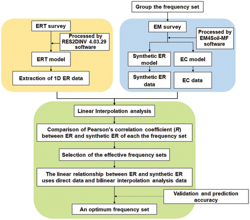
The optimum frequency set for FDEM surveys in the open dumpsite was evaluated by interpolation and linear regression (LR) between the ER and synthetic ER values. The synthetic ER values were created by inversion of the conductivity from the FDEM survey and the ER values were obtained by inversion of the apparent resistivity from the ERT survey. The selection of an optimum frequency set consisted of the following eight steps, as shown in Figure 3:

• The frequency sets were grouped using a sampling technique to arrange the frequency dataset, with each set containing three frequencies (the maximum number that can be measured by the EMP-400 profiler). The instrument has a frequency range from 1,000 to 15,000 Hz, which is divided into three groups: low frequency (1,000–5,000 Hz), moderate frequency (6,000–10,000 Hz), and high frequency (11,000–15,000 Hz). In this study, the frequency set was randomized into these different groups, with each profile containing 51 frequency sets, as listed in Table 1. Notably, we did not set groups entirely from the same frequency range, namely “Low–Low–Low”, “Moderate–Moderate–Moderate”, and High–High–High”, because similar frequency ranges in EM surveys will propagate waves through the waste layer at approximately the same depth; this will result in a lack of information at other levels and propagation through less of the subsurface medium, thus causing poorer data quality and increased difficulty in interpreting the EC distribution. These issues are similar to the problems encountered in single-frequency EM surveys (Kaufmann 2014; Hunkeler et al. 2015).

• EC data obtained from each frequency set were processed to generate the EC and synthetic ER models.

• Extraction of 1D ER data from the ERT survey was performed by selecting three-quarters of all the data points for comparison with synthetic ER values from the same intersection points and DOIs obtained from the interpolation analysis.

• Linear interpolation analysis was applied to obtain synthetic ER and ER data from the same investigational depth. Both datasets from the shallower EM survey (6–7 m depth) were used in the linear correlation analysis.

• Pearson’s correlation coefficient (R) was analyzed between the ER and synthetic ER data for each frequency set across all profiles.

• R values were compared between each frequency set to select effective frequency sets with high correlation coefficients (R ≥ 0.7).

• We evaluated and selected effective frequency sets with high correlation coefficients in all profiles.

• We analyzed the linear relationship between the synthetic ER data and ER data for each effective frequency set using data obtained from the direct collection and bilinear interpolation analysis; this process was used to determine the optimum frequency set for FDEM surveys in the open dumpsite.

Table 1. Arrangement of the frequency set of FDEM surveys.

Type	Name	f (kHz)	Type	Name	f (kHz)
Low–High–High	A1	1,10,15	Low–Low–Moderate	G1	1,3,6
	A2	1,11,15		G2	1,3,7
	A3	1,12,15		G3	1,3,8
	A4	1,13,15		G4	1,3,9
	A5	1,14,15		G5	1,3,10
	E1	2,11,15	Low–Low–High	C1	1,2,15
	E2	3,11,15		C2	1,3,15
	E3	4,11,15		C3	1,4,15
	E4	5,11,15		C4	1,5,15
	I1	1,11,13	Low–Moderate–Moderate	H1	1,7,9
	I2	1,10,13		H2	2,7,9
	I3	1,12,13		H3	3,7,9
	I4	1,14,13		H4	4,7,9
	I5	1,10,11		H5	5,7,9
	I6	1,12,11	Moderate–Moderate–High	D1	6,7,15
	I7	1,14,11		D2	6,8,15
Low–Moderate–High	B1	1,6,15		D3	6,9,15
	B2	1,7,15		D4	6,10,15
	B3	1,8,15		J1	7,8,15
	B4	1,9,15		J2	7,9,15
	K1	1,7,10	Moderate–High–High	F1	7,10,15
	K2	1,7,11		F2	7,11,15
	K3	1,7,12		F3	7,12,15
	K4	1,7,13		F4	7,13,15
	K5	1,7,14		F5	7,14,15
	K6	1,7,15

Figure 3. Flowchart showing the selection process of an optimum frequency set.

Interpolation analysis

Interpolation analysis is a statistical method used to predict the values of unknown data points based on known sample data. This method is currently applied in environmental science and geophysics fields such as altitude, depth, rainfall, and chemical concentration (Li and Heap 2014; Mariani and Basu 2015). In this, study, interpolation analysis was applied to decrease the limitations of LR analysis between ER data and synthetic ER data for different DOI; accordingly, the interpolation technique was applied to forecast the synthetic ER and ER data values for the same DOI. This study selected appropriate interpolation techniques based on the type of data (i.e., 1D or 2D data), with two interpolation analysis techniques applied (linear interpolation and bilinear interpolation) as follows:

• Linear interpolation is a common technique for creating new data points within the range of known data points using linear polynomials. This technique is suitable for one-dimensional data points and is effective for high-density data forecasting, especially for scientific applications (Li and Heap 2014; Mariani and Basu 2015). Thus, linear interpolation analysis was selected to forecast synthetic ER data at different DOI. This analysis technique allowed us to obtain synthetic ER values at the same depths as the 1D ER data, allowing the preliminary correlation between the datasets to be assessed. Linear interpolation analysis was calculated using the following relationship:

If the two known values are (x₁, y₁) and (x₂, y₂), then the y value for some point x is given by:

(4) $y=y_1+\left(x-x_1\right)\frac{y_2-y_1}{x_2-x_1}$(4)

where the coordinates of the first point are x₁ and y₁, the coordinates of the second point are x₂ and y₂, the point at which the interpolation is being performed is x, and the interpolated value is y.

• Bilinear interpolation is a popular approach for two-dimensional rectangular interpolation, especially in computer modeling and image processing. This technique extends the regular linear interpolation technique to approximate the function’s value at any point (x, y) within a 2D rectangle. This method assumes the values of some unknown function are known at each of the four corners of a rectangle; these coordinates are then set to (x₁, y₁), (x₁, y₂), (x₂, y₁), and (x₂, y₂) to find the unknown value (P) of the function at some location (x, y). The formula for calculating P is:

(5) $\begin{array}{rl}& P=\frac{\left(x_2-x\right)\left(y_2-y\right)}{\left(x_2-x_1\right)\left(y_2-y_1\right)}{Q}_{11}+\frac{\left(x-x_1\right)\left(y_2-y\right)}{\left(x_2-x_1\right)\left(y_2-y_1\right)}{Q}_{21}\\ & +\frac{\left(x_2-x\right)\left(y-y_1\right)}{\left(x_2-x_1\right)\left(y_2-y_1\right)}{Q}_{12}+\frac{\left(x-x_1\right)\left(y-y_1\right)}{\left(x_2-x_1\right)\left(y_2-y_1\right)}{Q}_{22}\end{array}$(5)

where the values of the function are known at four points: Q₁₁ is the value at (x₁, y₁), Q₂₁ is the value at (x₁, y₂), Q₁₂ is the value at (x₂, y₁), and Q₂₂ is the value at (x₂, y₂). Equation (4)(4) $y=y_1+\left(x-x_1\right)\frac{y_2-y_1}{x_2-x_1}$(4) indicates that bilinear interpolation is the weighted average of values Q₁₁, Q₁₂, Q₂₁, and Q₂₂ from the four corners of the rectangle, where the weights are based on the distance between the corners and the interpolation point (x, y). This is similar to the characteristics of electricity and electromagnetic waves that flow through the ground surface in the x-direction (horizontal) and y-direction (vertical), which can be interpolated to provide the apparent value at the surface to create a 2D model (Milsom 2003). Therefore, this study used bilinear interpolation to forecast synthetic ER data for each effective frequency set to compare with ER data at the same depth, thus allowing the optimum frequency set to be determined for FDEM surveys in open dump sites.

Pearson’s correlation analysis

Pearson’s correlation coefficient (or linear correlation) is a statistical method to determine the magnitude and direction of a linear relationship between two variables. This method gives a value (R) between −1 and 1, which can be interpreted as follows:

• A value close to 0 indicates no or very low correlation.

• Values close to 1 or −1 indicate a high degree of correlation.

The sign of the R value represents the direction of the relationship as either positive (direct variable) or negative (inverse) (Zhang 2016). This study used R to quantify the linear relationship between ER and synthetic ER for determining the optimum frequency set for FDEM surveying.

Validation and accuracy prediction

To assess the optimum frequency set, we predicted the accuracy of the EC model processed from each effective frequency set. The accuracy analysis of the EC model was evaluated using the RMSE and sensitivity analysis.

Root Mean Square Error (RMSE)

The RMSE is a popular statistical analysis tool to evaluate the conformity between simulated and measured values. This study used RMSE analysis to predict the accuracy of the EC model obtained from each effective frequency set, using the number of EC data points (around 670 for this analysis). The RMSE was estimated using the following formula:

(6) $RMSE=\sqrt{\frac{1}{N}\sum _{i=1}^N{({\sigma }_{ai}^o+{\sigma }_{ai}^c)}^2}$(6)

where ${\sigma }_{ai}^o$, ${\sigma }_{ai}^c$, and N are the measured apparent conductivity, the calculated apparent conductivity, and the number of data points, respectively. The smaller the RMSE value of an EC model, the better the consistency and the smaller the deviation between simulated and measured values and, therefore, the more accurate and reliable the model. In addition, the RMSE also effectively indicates the interpretability of the model’s simulated values (Abdennour et al. 2020).

Cumulative sensitivity analysis

Cumulative sensitivity (CS) analysis is used to evaluate the sensitivity of FDEM instruments for measuring any material above or below a specific depth. The CS value is defined as the relative contribution to the secondary magnetic field or the apparent conductivity from all material below a given depth (z) (Callegary, Ferré, and Groom 2007; Santos 2004).

In this study, we applied CS analysis for validation and accuracy prediction of selecting an optimum frequency set. This analysis compared the relationship between the standard CS values and the CS values of the effective frequency sets of all profiles. The calculated CS values from Equation (7)(7) $C{S}_{HCP}\left(z\right)=\underset{z}{\overset{\mathrm{\infty }}{\int }}L{S}_{HCP}\left(z\right)dz=\frac{1}{{(4z^2+1)}^{\frac{1}{2}}}$(7) and the actual z-values obtained from the field were used to calculate the standard CS values, and the CS value of the effective frequency series was calculated from the effective skin depth (z_e) in Equation (8)(8) $z_e=\frac{1}{5}\delta \approx \frac{100}{f\sigma }$(8) . The z_e parameter is equivalent to the local source skin depth, which is defined as the depth at which the amplitude of a local finite source’s electric or magnetic field in a homogeneous half-space decreases to e⁻¹ of its surface value (George et al. 2016).

The CS analysis for the horizontal coil orientation (CS_HCP), based on normal depth function (McNeill 1980), is calculated from the equations below:

(7) $C{S}_{HCP}\left(z\right)=\underset{z}{\overset{\mathrm{\infty }}{\int }}L{S}_{HCP}\left(z\right)dz=\frac{1}{{(4z^2+1)}^{\frac{1}{2}}}$(7)

(8) $z_e=\frac{1}{5}\delta \approx \frac{100}{f\sigma }$(8)

The cumulative sensitivity analysis consisted of five steps, as follows:

• Calculate the CS_HCP standard values for each profile from Equation (7)(7) $C{S}_{HCP}\left(z\right)=\underset{z}{\overset{\mathrm{\infty }}{\int }}L{S}_{HCP}\left(z\right)dz=\frac{1}{{(4z^2+1)}^{\frac{1}{2}}}$(7) using the z-values.

• Calculate the CS_HCP value of each effective frequency set using the z_e value obtained from Equation (8)(8) $z_e=\frac{1}{5}\delta \approx \frac{100}{f\sigma }$(8) .

• Use the CS_HCP value of each effective frequency set to calculate the average CS_HCP value.

• Evaluate the R value between the CS_HCP standard values and the average CS_HCP value of each frequency set across all survey lines.

• Compare and interpret the R values to select an optimum frequency set result and verify the validity and prediction of the study results.

Results and discussion

Electrical resistivity tomography survey results

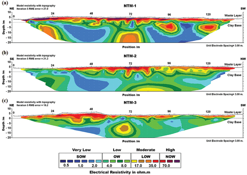
The ER model obtained from inversion modeling using RES2DINV 4.03.29 extends to a depth of approximately 20 m, as shown in Figure 4. The ER model shows homogeneous high electrical resistivity values within the waste layer, indicating that the waste has a high density and contains a high proportion of inorganic components (Ling et al. 2012; Feng et al. 2017). The RMSE values of the ERT models are 27.0, 21.3, and 19.2 for NTM-1, NTM-2, and NTM-3 respectively. A previous study by Georgaki et al. (2008) classified ER values and waste composition into four groups: (1) organic waste saturated with leachate (SOW); (2) organic waste (OW); (3) waste with very high inorganic content or with very low OW (LOW); and (4) entirely inorganic material (NOW). Accordingly, the ER model can be divided into three layers using this classification:

• The first layer has high resistivity (>50 Ω m) and extends approximately 5–7 m below the waste surface level. It has a typical thickness of around 5 m and forms a uniform layer in profiles NTM-1, NTM-2, and NTM-3, as shown in Figure 3. Georgaki et al. (2008) and Wangyao et al. (2019) suggest that high ER values (>50–300 Ω m) indicate the characteristics of accumulated old waste, such as less organic content, low moisture content, and high density; therefore, the first layer can be classified as NOW. This high-resistivity waste layer may also have a high plastic content.

• The second layer, with moderate resistivity (25–50 Ω m), occurs at a depth of approximately 6 m below the waste surface. This layer is thin (1–2.5 m) and forms a continuous layer under the uppermost high-resistivity layer throughout all three profiles. Field surveys show that the waste is relatively old, with leachate and rainwater seeping downward through a high-resistivity layer. Therefore, the waste in this layer is interpreted as saturated with water, resulting in moderately lower resistivity. The medium to high permeability of waste (approximately 10⁻⁶–10⁻⁴ m/s) (Durmusoglu, Sanchez, and Corapcioglu 2006) enables the downward movement of leachate and rainwater to accumulate in pores in the underlying clay base, which has lower permeability (approximately 10⁻¹⁰–10⁻⁹ m/s). As a result, some of the leachate cannot be drained and remains in the waste layer’s pores. This creates a saturated waste layer in which the electrical resistance is reduced, corresponding to Archie’s law, which states that electrical resistivity is inversely proportional to water saturation and porosity. For example, the waste layer saturated with the leachate is characterized by a low resistance but has high electrical conductivity.

• The third layer, with low resistivity (0.5–25 Ω m), is found at a depth of approximately 6–7 m from the surface. It is a continuous, thick layer situated beneath the moderate- and high-resistivity layers. In addition, low electrical resistivity values were found in the southeast of the NTM-2 and NTM-3 profiles, as shown in Figure 3. This low resistivity layer is interpreted as the geological base or clay base. The variable saturation within the clay layer produces heterogenous electrical resistivity across the study area.

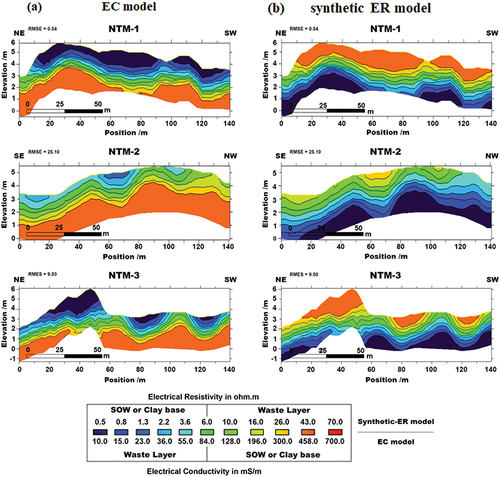
Figure 4. Inverted ERT model for profiles (a) NTM-1, (b) NTM-2, and (c) NTM-3. Adapted with permission from “Applying electromagnetic surveys as pre-screening tools prior to open dump mining,” by Boonsakul et al. (2021), J mater cycles waste manag 23, 1518–1530. Copyright (2021) by Springer Japan KK, part of Springer nature.

Electromagnetic survey results

The EC model obtained from inversion modeling using EM4Soil-MF software allows investigation at depths approximately 4–6 m below the surface, as shown in Figure 5. The distribution of EC values ranges from 10 mS/m to more than 100 mS/m. The observed distribution can broadly be divided into two layers:

• The first layer, with low to medium conductivity (10–100 mS/m) (Yannah et al. 2017), occurs from the surface of the waste to a depth of approximately 4 m. It is characterized as a uniform layer in profiles NTM-1 and NTM-3. This is consistent with previous studies by Yannah et al. (2017) and Crook, Levitt, and McNeill (2017), which indicate that old waste constituents (e.g., plastic, glass, rubber, and non-electromagnetic material) were found to have low EC values (<20 mS/m). These low values are due to their high inorganic content and low humidity, resulting in strong insulative properties and low electrical conductivity. The synthetic ER model of the first layer also showed moderate to high electrical resistivity (5–100 Ω m), as shown in Figure 5.

• The second layer has medium to high conductivity (over 100 mS/m) (Palacky 1988), corresponding to low electrical resistivity (approximately 0.5 Ω m) in the synthetic ER model. This thick layer was found under the first layer (low to medium EC layer) at subsurface depths exceeding 4 m. This layer can be interpreted as either waste saturated with leachate or the geological (clay) base. The study site’s leachate is known to have a high electrical conductivity of approximately 1,090–1,570 mS/m (Ogata et al. 2015), which would result in high electrical conductivity within this layer. A previous study (Soupios et al. 2007) identified that high subsurface conductivity values (40–150 mS/m) are associated with leachate saturation in landfills.

Figure 5. (a) Inverted EM results of the EC model, and (b) synthetic ER models obtained by inversion modeling of the conductivity data acquired from FDEM measurement along profiles NTM-1, NTM-2, and NTM-3. Adapted with permission from “Applying electromagnetic surveys as pre-screening tools prior to open dump mining,” by Boonsakul et al. (2021), J mater cycles waste manag 23, 1518–1530. Copyright (2021) by Springer Japan KK, part of Springer nature.

The selection and optimization of the frequency set

Pearson’s correlation coefficient analysis was performed between ER and synthetic ER data, with 148 data points (N = 148) compared to preliminarily assess the optimal frequency set for FDEM surveying. A relationship analysis revealed whether each profile had effective frequency sets, i.e., high-correlation frequency sets where R ≥ 0.7. The number of effective frequency sets in each profile, observed from the bar chart in Figure 6, is as follows:

• The NTM-1 profile had 34 effective frequency sets, as shown by the red bars in Figure 6.

• The NTM-3 profile had five effective frequency sets, as shown by the yellow bars in Figure 6.

• The NTM-2 profile did not have a high-correlation frequency set with R ≥ 0.7. However, around seven frequency sets for NTM-2 had a maximum correlation coefficient range of approximately 0.65–0.69, as shown by the blue bars in Figure 6.

Figure 6. Comparing the effective frequency sets of all profiles.

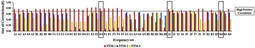
By comparing the effective frequency sets of all profiles, three sets were found to have very similar correlations, as shown by the black boxes in Figure 6. These are:

• The E4 frequency set, comprising 5,000 Hz, 11,000 Hz, and 15,000 Hz.

• The I1 frequency set, comprising 1,000 Hz, 11,000 Hz, and 13,000 Hz.

• The K4 frequency set, comprising 1,000 Hz, 7,000 Hz, and 13,000 Hz.

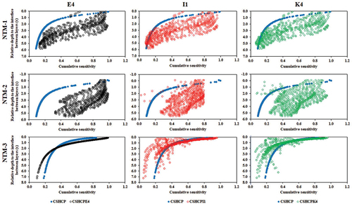
A scatter chart (Figure 7) shows the relationship between synthetic ER and ER data of all three effective frequency sets. It was found that:

• The NTM-1 profile had the following R values in the effective frequency sets:

Figure 7. Distribution of ER data and synthetic ER data from (a) direct correlation analysis, (b) linear interpolation analysis, and (c) bilinear interpolation analysis.

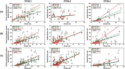
E4 = 0.79 (R² = 0.62), I1 = 0.76 (R² = 0.85), and K4 = 0.72 (R² = 0.52).

• The NTM-2 profile had the following R values in the effective frequency sets:

E4 = 0.69 (R² = 0.47), I1 = 0.67 (R² = 0.45), and K4 = 0.66 (R² = 0.44).

• The NTM-3 profile had the following R values in the effective frequency sets:

E4 = 0.70 (R² = 0.49), I1 = 0.67 (R² = 0.45), and K4 = 0.70 (R² = 0.49).

The linear relationships between the ER data and synthetic ER data for all three effective frequency sets were analyzed directly, with data also obtained by linear and bilinear interpolation. Each high-correlation frequency set used 48 data points for direct analysis and 148 data points generated from linear interpolation and bilinear interpolation analysis to determine the optimum frequency set for FDEM surveys in open dumpsites.

The results in Figure 7 indicate that the R values from direct correlation analysis (Figure 7a) are lower than those for the data from bilinear interpolation (Figure 7c), which provides a high to very high positive correlation. The R values of the three effective frequency sets analyzed from these two data sources produced the following results:

The correlation from data generated by direct correlation analysis had the R values in each profile as follows:

• The R values of profile NTM-1 are E4 = 0.65 (R² = 0.42), I1 = 0.57 (R² = 0.32), and K4 = 0.55 (R² = 0.30).

• The R values of profile NTM-2 are E4 = 0.22 (R² = 0.05), I1 = 0.24 (R² = 0.06), and K4 = 0.17 (R² =  0.03).

• The R values of profile NTM-3 are E4 = 0.71 (R² =  0.51), I1 = 0.66 (R² = 0.43), and K4 = 0.74 (R² = 0.55).

The correlation from data generated by bilinear interpolation had the R values in each profile as follows:

• The R values of profile NTM-1 are E4 = 0.91 (R² = 0.83), I1 = 0.85 (R² =  0.71), and K4 = 0.81 (R² = 0.65).

• The R values of profile NTM-2 are E4 = 0.74 (R² = 0.51), I1 = 0.72 (R² = 0.52), and K4 = 0.70 (R² = 0.49).

• The R values of profile NTM-3 are E4 = 0.83 (R² = 0.69), I1 =  0.74 (R² = 0.55), and K4 = 0.78 (R² = 0.61).

By comparing the data, it was found that the E4 frequency set (5,000, 11,000, and 15,000 Hz) was better distributed and achieved superior R values (between ER and synthetic ER) than the I1 and K4 frequency sets, as shown in Figures 7–8.

Figure 8. Comparison of the R values of the effective frequency sets E4, I1, and K4 in all three profiles.

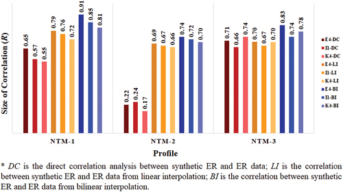
Based on the linear relationship analysis between ER and synthetic ER, when interpolation analysis was conducted to compare data at the same depth, the E4 frequency set achieved a higher positive correlation than the other frequency sets. The R values of the E4 frequency set obtained from direct correlation analysis show a positive correlation that ranges from low to high (R = 0.22–0.71), whereas the correlation analysis based on bilinear interpolation shows a positive correlation ranging from high to very high (R = 0.74–0.91).

In addition, the three statistical analysis approaches (i.e., direct analysis, linear interpolation, and bilinear interpolation) yielded different levels of correlation, as shown in Figure 8. The R values of data from bilinear interpolation indicated the strongest correlation (high to very high). Accordingly, this interpolation technique can be applied to estimate the best fit of 2D geophysical data; this approach also produces smoother transitions between data points when determining the optimum frequency set for FDEM surveying. While the linear interpolation technique yields moderate to strong positive correlation values (R = 0.69–0.79), it also has a lower R value than the bilinear method; this is likely because this study features extraction of 1D data from a 2D survey data for this statistical analysis, i.e., it is not an actual 1D survey, thus reducing the reliability of this interpolation approach.

In the direct linear correlation analysis between synthetic ER and ER data, key issues included the comparison of data at very different depths and the low number of data points (48) used for the analysis. These factors resulted in lower correlation values than those achieved using interpolation analysis. However, all three correlation analyses showed a similar correlation trend for the E4 frequency set; therefore, the E4 frequency set is considered to be the optimum frequency set for multi-frequency FDEM surveying of open dumpsites.

Validation and accuracy prediction results

The RMSE values of the EC model obtained through high-performance frequency set data processing are shown in Table 2. The results show that frequency set E4 had the lowest RMSE values than I1 and K4 frequency set, achieving RMSE values of NTM–1, NTM–2, and NTM–3. Therefore, the EC model obtained from inversion modeling using the E4 frequency set is the closest model to the true EC values from the study area.

Table 2. Degree of RMSE value and the correlation (R) between the CS_HCP standard values and the average CS_HCP values for the effective frequency sets for each profile.

Profiles	RMSE	R
NTM-1 E4	4.50	0.54
NTM-1 I1	37.90	0.52
NTM-1 K4	33.70	0.52
NTM-2 E4	25.10	0.46
NTM-2 I1	24.40	0.33
NTM-2 K4	38.50	0.30
NTM-3 E4	9.50	0.99
NTM-3 I1	17.60	0.87
NTM-3 K4	25.00	0.89

The CS analysis for horizontal coil orientations in the open dumpsite was investigated using the correlation between the standard CS values, calculated from the actual depth (z), and the CS values of the effective frequency set in each profile, calculated with z_e. The results indicate that the R values of NTM-1 display a moderate positive correlation (R = 0.52–0.54). Profile NTM-2 displays a low-to-moderate positive correlation (R = 0.30–0.46); however, profile NTM-3 exhibits a very strong positive correlation (R = 0.87–0.99). The RMSE and R values based on the CS values of all profiles are shown in Table 2.

By comparing the data, the E4 frequency set was found to have the highest R value across all profiles. Moreover, a significant trend between CS data and CS standard data was identified in one direction, as shown in Figure 9. This indicates that the E4 frequency set has superior sensitivity when used with the EMP-400 instrument profiler to evaluate waste composition at depth than the other tested frequencies.

Figure 9. Validation and accuracy prediction results showing the correlation between standard CS and CS values of the E4, I1, and K4 effective frequency sets across all profiles.

The validation and accuracy prediction results using both RMSE and CS analyses confirm that the E4 frequency set (5,000, 11,000, and 15,000 Hz) can be successfully employed to collect a weighted average complex conductivity value between the waste surface to the maximum investigated depth. Therefore, our findings demonstrate that E4 is the optimum frequency set for multi-frequency EM surveys for investigating waste composition in open dumpsites.

Conclusion

This study used multi-frequency EM surveys with 15 frequencies ranging from 1,000 to 15,000 Hz. Based on a range of analyses, a multi-frequency method containing frequencies of 5,000, 11,000, and 15,000 Hz effectively determined the waste composition and identified potential excavation points in open dumpsites for ODM operations. For these purposes, this approach was more effective than the single-frequency method. This study suggests that multi-frequency EM surveys are suitable as a screening tool before ERT surveying, as FDEM surveys provide better shallow-level survey data. These approaches also have the potential to identify LOW and NOW waste compositions suitable for RDF fuel production (such as plastic waste). These can be identified through their low electrical conductivity, corresponding to high electrical resistivity values in the ERT survey. In addition, multi-frequency EM surveys can improve the efficiency of conventional surveys for evaluating waste composition within an open dumpsite, such as reducing the number of required waste sampling sites by direct excavation and accurately identifying gas collection points for gas flux measurements. However, multi-frequency EM surveys have a limited investigation depth due to the fixed coil orientations of EM sensors.

To apply multi-frequency EM surveys at future disposal sites, FDEM surveying using the identified optimal frequency set should be compared with waste composition analysis, and 2D and 3D EM surveys should be conducted to create conductivity maps and 3D models of the final disposal site. It is beneficial to constrain the waste composition boundary and moisture content to determine a suitable area for in-depth exploration with ERT measurements. In addition, optimum frequency set investigations should be carried out in areas of other waste disposal methods (i.e., landfills) to assess solid waste composition. This approach can help to ensure the effectiveness of ODM and landfill mining operations in the future.

Acknowledgment

The authors would like to express their gratitude to The National Research Council of Thailand (NRCT), The Joint Graduate School of Energy and Environment (JGSEE), King Mongkut’s University of Technology Thonburi, and the Center of Excellence on Energy Technology and Environment (CEE), PERDO, and the Ministry of Higher Education, Science, Research and Innovation for the financial support provided to perform this study. They would also like to express gratitude to the Department of Earth Sciences, Faculty of Science, Kasetsart University, for supporting the instruments used during this research. In addition, the authors would like to thank the Nonthaburi Provincial Administrative Organisation and Siam Power Co., Ltd. for providing the study area.

Disclosure statement

No potential conflict of interest was reported by the author(s).

Data availability statement

The data that support the findings of this study are available from the corresponding author, [KW], upon reasonable request.

Additional information

Funding

This work was supported by the National Research Council of Thailand [7162].

Notes on contributors

Pornchanok Boonsakul

Pornchanok Boonsakul is a Ph.D. candidate at The Joint Graduate School of Energy and Environment, King Mongkut’s University of Technology Thonburi, Bangkok, Thailand.

Sasidhorn Buddhawong

Sasidhorn Buddhawong (Dr. rer. nat.) is an assistant professor at the School of Energy, Environment and Materials, King Mongkut’s University of Technology Thonburi, Bangkok, Thailand.

Komsilp Wangyao

Komsilp Wangyao (Ph.D.) is an assistant professor at The Joint Graduate School of Energy and Environment, King Mongkut’s University of Technology Thonburi, Bangkok, Thailand.

References

- Abdennour, M. A., A. Douaoui, C. Piccini, M. Pulido, A. Bennacer, A. Bradaï, J. Barrena, and I. Yahiaoui. 2020. Predictive Mapping of Soil Electrical Conductivity as a Proxy of Soil Salinity in South-East of Algeria. Environmental and Sustainability Indicators 8 (November):100087. doi:10.1016/j.indic.2020.100087.
- Barker, R. D. 1989. Depth of investigation of collinear symmetrical four‐electrode arrays. Geophysics 54 (8):1031–37. doi:10.1190/1.1442728.
- Bhatsada, A., S. Towprayoon, S. Garivait, K. Wangyao, T. Laphitchayangkul, and T. Ishigaki. 2020. Evaluation of UAV photogrammetric accuracy for mapping of open dump based on variation of image overlaps. KMUTT Res. Dev. J 25632:133–42.
- Bichet, V., E. Grisey, and L. Aleya. 2016. Spatial characterization of leachate plume using electrical resistivity tomography in a landfill composed of old and new cells (Belfort, France). Eng. Geol. 211:61–73. doi:10.1016/j.enggeo.2016.06.026.
- Boonsakul, P., S. Buddhawong, S. Towprayoon, S. Vinitnantharat, D. Suanburai, and K. Wangyao. 2021. Applying electromagnetic surveys as pre-screening tools prior to open dump mining. J. Mater. Cycles Waste Manage. 23 (4):1518–30. doi:10.1007/s10163-021-01232-5.
- Callegary, J., T. Ferré, and R. Groom. 2007. Vertical spatial sensitivity and exploration depth of low-induction-number electromagnetic-induction instruments. Vadose Zone J. 6 (1):158–67. doi:10.2136/vzj2006.0120.
- Carius, S., W. Hogland, L. Jilken, A. Mathiasson, and P. Andersson. 1999. A hidden waste material resource: Disposed thermoplastic. The 7th international waste management and landfill symposium, Sardinia, Italy.
- Cavalcante Fraga, L. H., C. Schamper, C. Noël, R. Guérin, and F. Rejiba. 2019. Geometrical characterization of urban fill by integrating the multi-receiver electromagnetic induction method and electrical resistivity tomography: A case study in Poitiers, France. Eur. J. Soil. Sci. 70 (5):1012–24. doi:10.1111/ejss.12806.
- Chiemchaisri, C., B. Charnnok, and C. Visvanathan. 2010. Recovery of plastic wastes from dumpsite as refuse-derived fuel and its utilization in small gasification system. Bioresour. Technol. 101 (5):1522–27. doi:10.1016/j.biortech.2009.08.061.
- Chiemchaisri, C., and C. Visvanathan. 2008. Greenhouse gas emission potential of the municipal solid waste disposal sites in Thailand. J. Air Waste Manage. Assoc. 58 (5):629–35. doi:10.3155/1047-3289.58.5.629.
- Chungam, B., S. Vinitnantharat, S. Towprayoon, D. Suanburi, S. Buddhawong, and K. Wangyao. 2021. Evaluation of the potential of refuse-derived fuel recovery in the open dump by resistivity survey prior to mining. J. Mater. Cycles Waste Manage. 23 (4):1320–30. doi:10.1007/s10163-021-01207-6.
- Crook, N., M. Levitt, and M. McNeill. 2017. Geophysical survey of the Los Angeles landfill, Albuquerque NM. Research report, HydroGeophysics Inc, USA.
- Deidda, G. P., M. Himi, I. Barone, G. Cassiani, and A. C. Ponsati. 2022. Frequency-domain electromagnetic mapping of an abandoned waste disposal site: A case in Sardinia (Italy). Remote Sens. 14 (4):878. doi:10.3390/rs14040878.
- Durmusoglu, E., I. M. Sanchez, and M. Corapcioglu. 2006. Permeability and compression characteristics of municipal solid waste samples. Environ. Geol. 50 (6):773–86. doi:10.1007/s00254-006-0249-6.
- Feng, S., Z. Bai, B. Cao, S. Lu, and S. Ai. 2017. The use of electrical resistivity tomography and borehole to characterize leachate distribution in Laogang landfill, China. Environ. Sci. Pollut. Res. 24 (25):20811–17. doi:10.1007/s11356-017-9853-0.
- Fraga, L. C., C. Schamper, C. Noël, R. Guérin, and F. Rejiba. 2019. Geometrical characterization of urban fill by integrating the multi‐receiver electromagnetic induction method and electrical resistivity tomography: A case study in Poitiers, France. Eur. J. Soil. Sci. 70:1012–24. doi:10.1111/ejss.12806.
- Georgaki, I., P. Soupios, N. Sakkas, F. Ververidis, E. Trantas, F. Vallianatos, and T. Manios. 2008. Evaluating the use of electrical resistivity imaging technique for improving CH (4) and CO (2) emission rate estimations in landfills. Sci. Total Environ. 389 (2–3):522–31. doi:10.1016/j.scitotenv.2007.08.033.
- George, N. J., D. N. Obiora, A. M. Ekanem, and A. E. Akpan. 2016. Approximate relationship between frequency-dependent skin depth resolved from geoelectromagnetic pedotransfer function and depth of investigation resolved from geoelectrical measurements: A case study of coastal formation, southern Nigeria. J. Earth Syst. Sci. 125 (7):1379–90. doi:10.1007/s12040-016-0744-4.
- Hunkeler, P. A., S. Hendricks, M. Hoppmann, S. Paul, and R. Gerdes. 2015. Towards an estimation of sub-sea-ice platelet-layer volume with multi-frequency electromagnetic induction sounding. Ann. Glaciol. 56 (69):137–46. doi:10.3189/2015AoG69A705.
- Isunza Manrique, I., D. Caterina, E. Van De Vijver, G. Dumont, and F. Nguyen. 2019. Assessment of geophysics as a characterization and monitoring tool in the dynamic landfill management (DLM) context : Opportunities and challenges. In Proceedings Sardinia 2019 : 17th International Waste Management and Landfill Symposium, Eds. R. Cossu, P. He, P. Kjeldsen, Y. Matsufuji, and R. Stegmann Santa Margherita di Pula, Cagliari, Italy: CISA Publisher.
- Kaufmann, M. S. 2014. Pseudo 2D inversion of multi-frequency coil-coil FDEM data. Master thesis., IDEA League, ETH Zurich, Switzerland.
- Kaya, M., G. Özürlan, and E. Şengül. 2007. Delineation of soil and groundwater contamination using geophysical methods at a waste disposal site in Çanakkale, Turkey. Environ. Monit. Assess. 135 (1–3):441–46. doi:10.1007/s10661-007-9662-x.
- Kondracka, M., I. Stan-Kłeczek, S. Sitek, and D. Ignatiuk. 2021. Evaluation of geophysical methods for characterizing industrial and municipal waste dumps. Waste Manag. 125:27–39. doi:10.1016/j.wasman.2021.02.015.
- Li, J., and A. D. Heap. 2014. Spatial interpolation methods applied in the environmental sciences: A review. Environ. Model. Softw. 53:173–89. doi:10.1016/j.envsoft.2013.12.008.
- Ling, C., Q. Zhou, Y. Xue, Y. Zhang, R. Li, and J. Liu. 2012. Application of electrical resistivity tomography to evaluate the variation in moisture content of waste during 2 months of degradation. Environ. Earth Sci. 68 (1):57–67. doi:10.1007/s12665-012-1715-y.
- Loke, M. H. 2000. Electrical imaging s surveys for environmental and engineering studies, a practical guide to 2-d and 3-d surveys. Malaysia: Penang.
- Maheshi, D., V. P. Steven, and V. Karel. 2015. Environmental and economic assessment of open waste dump mining in Sri Lanka. Resour. Conserv. Recyl. 102:67–79. doi:10.1016/j.resconrec.2015.07.004.
- Maio, R. D., S. Fais, P. Ligas, E. Piegari, R. Raga, and R. Cossu. 2018. 3D geophysical imaging for site-specific characterization plan of an old landfill. Waste Manag. 76:629–42. doi:10.1016/j.wasman.2018.03.004.
- Mariani, M. C., and K. Basu. 2015. Spline interpolation techniques applied to the study of geophysical data. Physica A 428:68–79. doi:10.1016/j.physa.2015.02.014.
- McNeill, J. 1980. Electromagnetic terrain conductivity measurement at low induction numbers. Tech. Note TN-6, Geonics Ltd, Ontario, Canada.
- Milsom, J. 2003. Field geophysics. 3rd ed. New York, USA: John Wiley & Sons.
- Ogata, Y., T. Ishigaki, Y. Ebie, N. Sutthasil, C. Chiemchaisri, and M. Yamada. 2015. Water reduction by constructed wetlands treating waste landfill leachate in a tropical region. Waste Manag. 44:164–71. doi:10.1016/j.wasman.2015.07.019.
- Osinowo, O., M. O. Falufosi, and E. O. Omiyale. 2018. Integrated electromagnetic (EM) and electrical resistivity tomography (ERT) geophysical studies of environmental impact of Awotan dumpsite in Ibadan, southwestern Nigeria. J. Afr. Earth Sci. 140:42–51. doi:10.1016/j.jafrearsci.2017.12.026.
- Palacky, G. 1988. 3. Resistivity characteristics of geologic targets. Electromagnetic methods in applied geophysics-theory, ed. M. N. Nabighian, 53–129. Tulsa, OK: Society of exploration geophysicists. doi:10.1190/1.9781560802631.ch3.
- Piero Deidda, G., L. de Carlo, M. Clementina Caputo, and G. Cassiani. 2022. Frequency domain electromagnetic induction imaging: An effective method to see inside a capped landfill. Waste Manag. 144 (February):29–40. doi:10.1016/j.wasman.2022.03.007.
- Prechthai, T., M. Padmasri, and C. Visvanathan. 2008. Quality assessment of mined MSW from an open dumpsite for recycling potential. Resour. Conserv. Recyl. 53 (1–2):70–78. doi:10.1016/j.resconrec.2008.09.002.
- Ramalho, E., A. C. Dill, and R. Rocha. 2012. Assessment of the leachate movement in a sealed landfill using geophysical methods. Environ. Earth Sci. 68 (2):343–54. doi:10.1007/s12665-012-1742-8.
- Rosendal, R. 2009. Landfill mining - process, feasibility, economy, benefits and limitations. Copenhagen, Denmark: RenoSam.
- Rosquist, H., V. Leroux, T. Dahlin, M. Svensson, M. Lindsjö, C. Månsson, and S. Johansson. 2011. Mapping landfill gas migration using resistivity monitoring. Waste Resour. Manag. 164 (1):3–15. doi:10.1680/warm.2011.164.1.3.
- Santos, F. A. 2004. 1-D laterally constrained inversion of EM34 profiling data. J. Appl. Geophys. 56 (2):123–34. doi:10.1016/j.jappgeo.2004.04.005.
- Sharma, A., R. Ganguly, and A. Kumar Gupta. 2018. Matrix Method for Evaluation of Existing Solid Waste Management System in Himachal Pradesh, India. Journal of Material Cycles and Waste Management 20 (3):1813–31. doi:10.1007/s10163-018-0703-z.
- Sharma, A., R. Ganguly, and A. Kumar Gupta. 2019. Characterization and Energy Generation Potential of Municipal Solid Waste from Nonengineered Landfill Sites in Himachal Pradesh, India. Journal of Hazardous, Toxic, and Radioactive Waste 23 (4):04019008. doi:10.1061/(asce)hz.2153-5515.0000442.
- Shemang, E., and K. Mickus. 2011. Geophysical characterization of the abandoned Gaborone landfill, Botswana: Implications for abandoned landfills in arid environments. Int. J. Environ. Prot. 1:1–12.
- Soupios, P., and D. Ntarlagiannis. 2017. Characterization and monitoring of solid waste disposal sites using geophysical methods: Current applications and novel trends. In Modelling trends in solid and hazardous waste managemen, ed. S. Debashish and A. Sudha, 75–103. Singapore: Springer Singapore. doi:10.1007/978-981-10-2410-8_5.
- Soupios, P., N. Papadopoulos, I. Papadopoulos, M. Kouli, F. Vallianatos, A. Sarris, and T. Manios. 2007. Application of integrated methods in mapping waste disposal areas. Environ. Geol. 53 (3):661–75. doi:10.1007/s00254-007-0681-2.
- Wangyao, K., N. Sutthasil, and C. Chiemchaisri. 2021. Methane and nitrous oxide emissions from shallow windrow piles for biostabilisation of municipal solid waste. J. Air Waste Manage. Assoc. 71 (5):650–60. doi:10.1080/10962247.2021.1880498.
- Wangyao, K., S. Towprayoon, K. Koetrit, A. Phongphiphat, and K. Boonrod. 2019. Applications of geophysics in landfill mining business for refuse derived fuel production. Final report, National Research Council of Thailand, Bangkok.
- Xaypanya, P., J. Takemura, C. Chiemchaisri, H. Seingheng, and M. A. N. Tanchuling. 2018. Characterization of landfill leachates and sediments in major cities of Indochina Peninsular countries—heavy metal partitioning in municipal solid waste leachate. Env. MDPI 5 (6):1–24. doi:10.3390/environments5060065.
- Yannah, M., K. Martens, M. V. Camp, and K. Walraevens. 2017. Geophysical exploration of an old dumpsite in the perspective of enhanced landfill mining in Kermt area, Belgium. Bull. Eng. Geol. Environ. 78 (1):55–67. doi:10.1007/s10064-017-1169-2.
- Zhang, Z. 2016. Environmental data analysis: Methods and applications. Germany: Walter de Gruyter GmbH.