Development and validation of a route planning methodology for vehicle-based remote measurements of methane and other emissions from oil and gas wells and facilities

ABSTRACT

Multi-sensor vehicle systems have been implemented in large-scale field programs to detect, attribute, and estimate emissions rates of methane (CH₄) and other compounds from oil and gas wells and facilities. Most vehicle systems use passive sensing; they must be positioned downwind of sources to detect emissions. A major deployment challenge is predicting the best measurement locations and driving routes to sample infrastructure. Here, we present and validate a methodology that incorporates high-resolution weather forecast and geospatial data to predict measurement locations and optimize driving routes. The methodology estimates the downwind road intersection point (DRIP) of theoretical CH₄ plumes emitted from each well or facility. DRIPs serve as waypoints for Dijkstra’s shortest path algorithm to determine the optimal driving route. We present a case study to demonstrate the methodology for planning and executing a vehicle-based concentration mapping survey of 50 oil and gas wells near Pecos, Texas. Validation was performed by comparing DRIPs with 174 CH₄ plumes measured by vehicle surveys of oil and gas wells and facilities in Alberta, Canada. Results indicate median Manhattan distances of 145.8 m between DRIPs and plume midpoints and 160.3 m between DRIPs and peak plume enhancements. A total of 46 (26%) of the plume segments overlapped DRIPs. Locational errors of DRIPs are related to misattributions of emissions sources and discrepancies between modeled and instantaneous wind direction measured when the vehicle intersects plumes. Although the development of the methodology was motivated by CH₄ emissions from oil and gas facilities, it should be applicable to other types of point source air emissions from known facilities.

Implications: This paper presents and validates a method that addresses the challenge of measuring industrial emissions from public roads. The method can increase the effectiveness and efficiency of targeted vehicle-based emissions surveys where the locations of potential sources are known. We believe the method has broad application in addition to the upstream oil and gas context it was designed for.

Introduction

Reducing methane (CH₄) emissions from industrial sources such as the oil and gas sector is a major focus of new government regulations, initiatives, and voluntary industry actions to mitigate climate change (e.g., AER 2020; CDPHE 2019; ECCC 2018; EU 2020; NMED 2020; PDEP 2019; US EPA 2021). CH₄ is invisible and odorless in the upstream and midstream sectors of the oil and gas supply chain, which makes it difficult to detect and reduce without specialized sensing technology. Conventional technologies and methods to detect CH₄ emissions from oil and gas operations rely on handheld instruments such as organic vapor analyzers (OVAs) and optical gas imaging (OGI) cameras (US EPA 2017). These technologies and related work practices are effective at locating emissions sources, tagging emitting components, and directing repairs. However, these close-range methods are time-consuming because there are many potential component sources at each site that must be inspected. The number of oil and gas wells and facilities is very numerous in some regions (e.g., up to 56 oil wells per km² in the Permian Basin; Scanlon et al. 2017). To help address this, a range of alternative technologies have been developed with the goal of more efficiently detecting CH₄ emissions and guiding follow-up. The suite of new technologies that fall into this category includes mobile platforms such as satellites, drones, vehicle systems, aircraft, and fixed sensors. Since these technologies generally lack the spatial resolution to identify component-level emissions, they are referred to as screening tools (Fox et al. 2019, 2021).

Vehicle-based systems are an established technology for detecting, attributing, and quantifying CH₄ emissions from wells and facilities (Fox et al. 2019). These systems typically integrate sensors for measuring the CH₄ mixing ratio, wind, and vehicle location, and work practices defining how measurements are collected for specific purposes such as concentration mapping, source characterization, and emissions quantification (Albertson et al., 2016; Barchyn and Hugenholtz 2022; Brantley et al. 2014; Phillips et al. 2013; Yacovitch et al. 2015; Zhou et al. 2021). To date, multi-sensor vehicle systems have been successfully adopted worldwide (Al-Shalan et al. 2022; Atherton et al. 2017; Defratyka et al. 2021; Maazallahi et al. 2020; Maher, Santos, and Tait 2014; Sun et al. 2019; Yacovitch et al. 2018; Zavala-Araiza et al. 2018; Zazzeri et al. 2015) to measure various types of CH₄ emission sources under both urban and non-urban environments (von Fischer et al. 2017; Zazzeri et al. 2017; Zhou et al. 2019; Ars et al. 2020; Robertson et al. 2020; Weller, Hamburg, and von Fischer 2020; Bakkaloglu et al. 2021; Lu et al. 2021). In addition, vehicle systems have standardized and well tested work practices, which define how measurements are collected and processed into information (e.g., United States Environmental Protection Agency (EPA) Other Test Method 33A; (Brantley et al. 2014; 2015; Robertson et al. 2017; Edie et al. 2020).

However, because these systems must intersect plumes to detect enhancements of CH₄ (ΔCH₄), either while driving or parked, their effectiveness for measuring CH₄ emissions is strongly modulated by road access that is immediately downwind of the emissions source. Plumes are undetectable when the vehicle is upwind of the source. For routine monitoring surveys or larger-scale campaigns, strategic route planning could be used to maximize plume intersection probability as a function of road network and wind conditions. By increasing the probability of detecting plumes from target sources, crews can reduce windshield time, associated risks, and ancillary vehicle emissions of CO₂.

This article builds on the path planning approach outlined in Albertson et al. (2016) by developing a reproducible and validated methodology to estimate the most effective and efficient driving route for measuring CH₄ emissions from wells and facilities. The methodology applies a series of geospatial procedures to high-resolution weather forecast data, well/facility points, and road network data. An example from the Permian Basin demonstrates the operationalization of the method for route planning under time-varying wind direction. Validation is performed using mobile measurements of 174 CH₄ plumes attributed to oil and gas wells and facilities in Alberta, Canada.

Methodology

Downwind road intersection point (DRIP)

The methodology was developed to support operational research and monitoring activities at a regional scale with vehicle-based measurements from public roads. The basis for this approach is to enable measurements at a stand-off distance where the plume is well mixed, and to avoid the need for direct access to wells or facilities, which typically requires permission and coordination with the facility operator. The main output of the methodology is an estimate of the shortest (optimal) driving route from a point of origin to a series of waypoints and return to the point of origin. Each waypoint corresponds to a downwind road intersection point (DRIP) that approximates the location where a theoretical plume of CH₄ emitted from an oil and gas well or facility advects over a road. Therefore, DRIPs represent the locations where a vehicle system has the best chance of measuring a plume.

Three input datasets are needed to estimate DRIPs: forecast wind direction, well or facility point locations, and road networks. To estimate wind, we use gridded high-resolution weather forecasts, such as the 2.5 km resolution High Resolution Deterministic Prediction System (HRDPS) from Environment and Climate Change Canada (Milbrandt et al. 2016), and the 3 km resolution High-Resolution Rapid Refresh (HRRR) model from the U.S. National Oceanic and Atmospheric Administration (Benjamin et al. 2016). Other gridded forecast datasets from the European Center for Medium-Range Weather Forecasts (ECWMF), can be used for regions outside North America. These datasets provide hourly estimates of near-surface (10 m) meridional ($v$) and zonal ($u$) wind components, which are converted to wind direction ($\theta$):

(1) $\theta =180+\frac{180}{\pi }atan2\left(u,v\right)$(1)

Archival HRDPS and HRRR data are available from the Canadian Surface Prediction Archive (CaSPAr; Mai et al. 2020) and the University of Utah (Blaylock, Horel, and Liston 2017). Well and facility locations are available from provincial or state-level data, such as the Alberta Energy Regulator’s ST37 and ST102 datasets, or national-level data such as the US Homeland Infrastructure Foundation-level Data (HIFLD). Road data are available from OpenStreetMap (OSM; Haklay and Weber 2008) or other infrastructure databases.

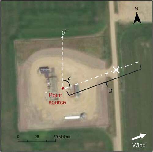
DRIPs are estimated by extending a virtual line downwind of a well or facility point location until it intersects the nearest public road (Figure 1). This virtual line represents the best estimate available of a time-averaged plume centreline emanating from the well or facility point under a constant wind direction. The virtual line can extend downwind by a pre-defined distance threshold, but the effective distance for detection varies according to the emission rate, terrain, weather conditions, and vehicle system characteristics such as the measurement rate, resolution, and driving speed. At some distance downwind, plumes are diluted and undetectable against the background CH₄ mixing ratio. The literature indicates that most vehicle-based measurements of CH₄ emissions are acquired from distances of a few decameters up to several kilometers downwind of oil and gas wells and facilities (e.g., 20–200 m in OTM33A; 40–1200 m in Lan et al. 2015; ~700 m in Yacovitch et al. 2017; < 300 m in Caulton et al. 2018; 500–2000 m in Zhou et al. 2019). Next, the latitude and longitude of the intersection between the virtual line and the nearest downwind road are converted to a point – this is the DRIP. Finally, DRIPs serve as waypoints for Dijkstra’s algorithm (Dijkstra 1959), which applies weights based on the speed limit of road segments between two connected points to find the shortest or lowest cost driving route.

Figure 1. Illustration of the downwind road intersection point (DRIP). The red dot represents the center of an O&G facility pad and a location of a potential point emission source, α is the downwind direction at the source location relative to true north, D is the user-defined length of the line segment, and X is the DRIP. Wind is from the southwest to the northeast.

Implementation

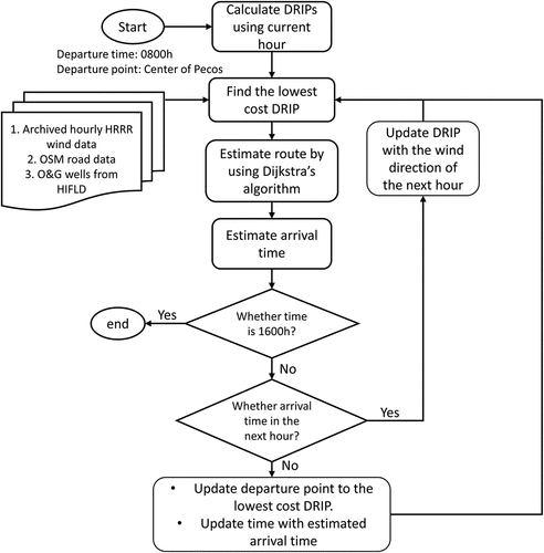
One of the challenges for implementing the methodology is that the wind direction changes with time, which means that DRIP locations are dynamic. Therefore, routes must be updated at timescales that are consistent with the input wind forecast data to account for changes in DRIP locations. To operationalize the methodology, we developed a simulation of route optimization for a hypothetical concentration mapping survey of 50 randomly selected oil and gas wells within 50 km of Pecos, Texas, USA, on 18 September 2021. The input datasets consisted of archived hourly HRRR wind forecast data, public roads from OSM, and point locations of oil and gas wells from the HIFLD. The simulation involved seven steps (Figure 2). First, DRIPs were calculated from archived hourly HRRR wind forecast data for each oil well at the beginning of the survey (0800 h local time). A distance threshold of 2 km was used for the virtual lines extending downwind from the well site points. Second, the lowest cost (shortest travel time) DRIP from the departure point (geographic center of Pecos) was determined at the start of the survey by iteratively applying Dijkstra’s algorithm and speed limit weighting to all 50 DRIPs. The lowest cost DRIP was set as the first waypoint of the survey (WP1). Third, the arrival time from the departure point to WP1 was estimated using the speed limit of the intervening road segments. Fourth, if the estimated time of arrival was in the next hour, the DRIP location for WP1 was recalculated based on the forecast wind direction of the next hour, otherwise the original DRIP location was used as WP1. Fifth, the route was updated if the location of WP1 changed from the original estimate. Sixth, steps 1–4 were repeated using the last DRIP as the departure point until the time reached 1600 h, which was arbitrarily chosen at the end of the survey. Finally, the lowest cost route from the last DRIP to the original departure point was calculated.

Figure 2. Flowchart of route planning with temporally- and spatially-varying forecast wind direction.

Validation

The methodology was evaluated using real vehicle-based measurements of CH₄ emissions from oil and gas wells and facilities in Alberta, Canada. We evaluated the spatial accuracy of the DRIPs by comparing the estimated locations with actual CH₄ plumes measured by the University of Calgary vehicle system, called PoMELO (Barchyn and Hugenholtz 2022). PoMELO fuses data from three sensors: (i) an open-path methane sensor (Li-Cor LI-7700), (ii) a global navigation satellite system (GNSS) (Hemisphere V112), and (iii) a 2D sonic anemometer (RM Young 86000). Measurements of the CH₄ mixing ratio, location, and wind speed and direction were recorded at 10 Hz. The wind data were corrected for vehicle speed and aerodynamic effects by subtracting the induced motion from wind measurements after accounting for the aerodynamic influence of the vehicle. Surveys were performed in the summer of 2018 and winter of 2020 for an unrelated research project assessing PoMELO’s hardware and software performance. From the raw data, 174 well-defined plumes were extracted using the segmentation procedure outlined by Barchyn, Hugenholtz, and Fox (2019). The segmentation procedure finds the global mixing ratio maxima and iteratively “grows” the segmented plume within the time series by connecting regions of locally elevated methane. The 174 plumes were selected from approximately 890 unknown source plumes using a two-stage process (Figure 3). First, each plume segment was referenced to well or facility points obtained from the Alberta Energy Regulator’s ST37 or ST102 datasets, available open access satellite imagery, and wind direction data from PoMELO (Figure 3a). PoMELO plume segments that did not appear to be associated with upwind oil and gas wells or facilities, and those > 1 km from the nearest upwind well or facility point, were excluded. Next, from this subsample, we extracted the wind direction from each PoMELO plume segment and created two upwind-facing wind wedges with the apexes located at the center of the segment (Figure 3b). The first upwind-facing wind wedge was created using the range of wind direction measurements from each segment, and the second was created using wind directions at the peak ΔCH₄ and the midpoint of plume segment. The second, narrower wind wedge was only used in a handful of cases where two wells or facilities were located within the first wind wedge. In these cases, the second wind wedge was used to identify the facilities or wells that were most likely the source of the emissions. The result was a sample size of 174 plume segments attributed to upwind oil and gas facilities and wells: 164 from surveys in 2018 and 10 from surveys in 2020. Because we did not visit each well or facility to confirm they were the source of the detected emissions, we refer to these as suspected sources.

Figure 3. Overview of the validation methodology. (a) CH₄ mixing ratio measurements along a road with the wind direction denoted by the small arrows. (b) After the plume is segmented, two wind wedges are extracted from the vehicle’s wind measurements to verify that a facility or well point is located within one or the other. (c) Once the DRIP is determined the road distance to the peak CH₄ and plume midpoint are measured to determine spatial errors. (d) A line graph showing the CH₄ mixing ratio vs distance where 0 m is the north end of the plume. The driving speed for this sample case is about 67 km/hour.

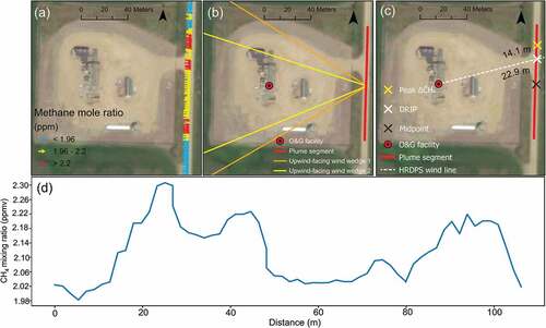
Archived hourly wind data from the HRDPS were retrieved from the CaSPAr platform (Mai et al. 2020) for the dates and times corresponding to the 174 plume segments. The HRDPS-derived wind directions from the same hour as the vehicle measurements were used to estimate the location of each DRIP. We individually inspected the accuracy of DRIPs by overlaying the sampled plume segment, the attributed O&G or facility or well, HRDPS-derived wind directions, midpoints of plume segments, and two corresponding upwind-facing wind wedges with satellite imagery in ArcGIS Pro. The spatial error was based on the Manhattan (road) distance ($d_M$) between the DRIPs and the corresponding plume segment midpoint and between the DRIPs and the peak ΔCH₄ of the corresponding plume segment (Figure 3c). The Manhattan distance ($d_M$) represents the one-norm (sum of absolute values) of the distance between two points measured along roads. The formula for calculating the Manhattan distance between points A at ($x_1,y_1$) and B at ($x_2,y_2$) can be expressed as follow:

(2) $d_M=\left|x_1-x_2\right|+\left|y_1-y_2\right|$(2)

Results and discussion

Operational deployment demonstration

xThe wind field over the study region varied on 18 September 2021, which highlights the importance of using high-resolution gridded forecast wind data to estimate and update DRIPs during the survey period (Figure 4). A single wind direction applied to estimate DRIPs at all 50 target well sites would not capture the spatial and temporal variability observed in the HRRR forecast data. To illustrate the estimated DRIPs and route, we divided the survey into roughly 1-hour segments, which are shown in the panels in Figure 4. The first well site surveyed in each segment is labeled “A”, followed by the next site labeled “B”, and so on. The route shown in each segment begins at the last DRIP surveyed in the previous segment. Each segment shows DRIPs and routes based on the forecast wind direction in the hour the well sites are expected to be surveyed based on the estimated driving time.

Figure 4. Operational demonstration of the methodology. The optimal route (green line) for 50 randomly selected oil and gas wells within 50 km of Pecos, Texas, USA, on 18 September 2021 is shown in panel (a). Panels (b-i) show the optimized routes for different time segments of the survey based on the estimated travel time. Wells are represented by colored points and labeled (A, B, C, …) according to the order they are surveyed in each segment. Subscript digits denote the corresponding time segment. Blue points are wells that were not surveyed because they did not have a DRIP located within 2 km downwind or their DRIPs were not included in the optimal route. Green points are wells that were surveyed because they had a DRIP located within 2 km downwind. Red points are wells surveyed in the specified survey segment. DRIPs are denoted by the red x’s. Black arrows are 2 km virtual lines calculated using the average of the two wind directions associated with the period displayed in the panel.

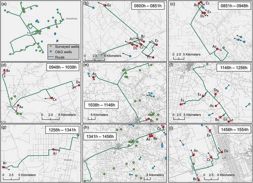
The simulation indicates the concentration mapping survey would have covered 34 of the 50 target wells (68%). The 16 wells not covered by the survey were too far upwind (> 2 km) of the estimated DRIPs. The total (shortest) driving distance to cover the 34 wells was 537.4 km, which is one well surveyed every 14 minutes or every 15.8 km on average. Given the high density of wells in this region, we anticipate the ratio of wells surveyed per km of driving and the total number of wells covered would be much higher if the sample size was larger.

Arrival times at each waypoint were estimated in the simulation based on the assumption the vehicle traveled at the speed limit. However, the practical extension is to update the driving route based on vehicle location and time, which are derived from an onboard GNSS receiver. This accounts for delays during the survey from vehicle traffic or stops and re-routing from road construction or other route deviations. To demonstrate this practical implementation, we integrated GNSS data with OSM, Dijkstra’s algorithm, and hourly estimates of DRIP locations calculated with HRDPS forecast wind data. We conducted a fictitious survey of emissions sources in Coquitlam, British Columbia on 25 November 2021. DRIP locations were automatically updated when the local time transitioned from one hour to the next. The driving route was also automatically updated by applying Dijkstra’s algorithm at 1 second intervals, which accounted for route deviations and changes in DRIP locations. A video showing route updates based on vehicle location, time, and changes in DRIP locations from the survey is presented by Gao (2021).

Validation

We compared DRIPs with 174 CH₄ plumes measured by PoMELO (Supplementary Data). The plume segments derived from the PoMELO vehicle measurements ranged in length from 7.1 m to 928.3 m with a mean and median of 128.1 m and 68.0 m, respectively. The frequency distribution is right skewed, indicating a tendency for shorter plume segments in the sample (Figure 5a). The Euclidian distance between suspected sources and plume midpoints (peak ΔCH₄) was right skewed, ranging from 15.1 m (15.1 m) to 946.8 m (934.3 m) with a mean and median of 235.7 m (239.2 m) and 157.9 m (159.7 m), respectively. The average Manhattan distance between the plume midpoint and peak ΔCH₄ was 27.5 m. More than 60% of the 174 plume midpoints were within 200 m of source points, which is the upper distance limit recommended for use of OTM33A (Thoma and Squier 2014).

Figure 5. Validation results of DRIPs. (a) Box plots of plume lengths, the Euclidean distance between suspected sources and plume midpoints, the Euclidean distance between suspected sources and plume peak ΔCH₄, and the Manhattan distance between plume midpoints and plume peak ΔCH₄. (b) A histogram of the Manhattan distance between DRIPs and plume midpoints by landcover types (logarithmic scale). (c) A histogram of the Manhattan distance between DRIPs and plume peak ΔCH₄ by landcover types (logarithmic scale). (d) A scatterplot between the HRDPS wind speed for each site and the average wind speed measured by PoMELO for each plume segment with colors indicate the standard deviation of wind directions measured by PoMELO.

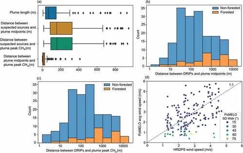
Manhattan distances between 174 DRIPs and the corresponding plume midpoints and peak ΔCH₄ derived from vehicle measurements are shown in Figure 5(c,d). The heavy-tailed frequency distributions indicate a tendency for shorter Manhattan distances. The median Manhattan distance between DRIPs and plume midpoints was 145.8 m, and 160.3 m between DRIPs and peak ΔCH₄. The 25^th and 75^th quartiles were 46.1 m and 810.0 m between DRIPs and plume midpoints, and 46.8 m and 810.0 m between DRIPs and peak ΔCH₄. A total of 46 (26%) plume segments overlapped DRIPs. Half of all plume midpoints and peak ΔCH₄ were < 8 seconds to the nearest DRIPs based on the road speed limits.

When the spatial error was assessed by landcover type, the Manhattan distance increased substantially in forest settings, which may be partly an effect of the lower density and irregular configuration of roads compared to those in the regions dominated by agriculture. A total of 33 (19%) of the DRIPs were in forest settings, while 141 (81%) were in settings dominated by grassland and crop agriculture. The median Manhattan distance was 781.7 m between 33 DRIPs in forest settings and the corresponding plume midpoints and peak ΔCH₄. Four DRIPs in forest settings were > 7.5 km from the corresponding plume midpoints and peak ΔCH₄. In agriculture settings, where the road network is gridded, the median Manhattan distance between 141 DRIPs and plume midpoints was 105.5 m, and 111.4 m between DRIPs and peak ΔCH₄. While the sample sizes are not equivalent, data suggest the method may be less reliable in forest settings.

Two main factors affect the spatial error of DRIPs. First, there is error in the location of DRIPs from the misattribution of emission source locations. Because we did not directly identify the component- or equipment-level sources of each plume, it possible that emissions came from sources that did not coincide with the locations of the well and facility points used to estimate the DRIPs. This is particularly important for oil and gas facilities that have multiple pieces of equipment and potential emissions sources spread over an area on pads, such as tanks, flare stacks, separators, engine exhausts, well heads and risers, compressors, and surface casing vents. Whereas DRIPs are calculated from a single point for each well and facility, often there are several pieces of equipment on each pad that could be emitting. This source of error is less important as the distance increases from source to DRIP.

Second, the forecast wind data does not capture horizontal wind variability at the spatial and temporal scales of the vehicle measurements, or wind modifications from interactions with near-surface features and terrain. The vehicle measurements captured instantaneous features of plumes and wind conditions near ground level, whereas the forecast data and DRIPs were based on a more generalized or time-averaged representation of wind conditions at 10 m a.g.l. and inferred plume behavior. The result is that plume behavior at instantaneous timescales, like meandering, can produce spatial offsets in the concentration field relative to the time-averaged centerline, particularly during low wind speeds associated with weak large-scale flow (e.g., Mahrt 2011). Wind direction errors preferentially impact DRIPs that are further downwind from the source due to geometry; however, at further downwind distances the plume more closely reflects the longer timescale average wind direction. This may account for some of the difference between the DRIPs and corresponding plume midpoints and peak ΔCH₄ locations. Additionally, the forecast models do not incorporate local terrain and roughness features that may result in deviations of wind direction and DRIP locations relative to the plumes. The average percentage difference between HRDPS wind speed for each site and the PoMELO average wind speed for each plume segment was 40% (Figure 5d), which reveals a limitation of the forecast wind data. Figure 5(d) also shows that the standard deviation of the wind direction measured by PoMELO is higher when the measured wind speed is less than 1 m/s. Therefore, sufficient wind speeds (>1 m/s) are required to maximize the accuracy of the DRIPs. However, this should not significantly impact the results of the route planning in most cases.

Conclusion

This study developed a geospatial method to optimize vehicle routing for measuring methane emissions from oil and gas wells and facilities. The method integrated the emission source location, road network, and forecast wind direction to maximize the probability of plume intersection (DRIPs) for regional surveys. We first demonstrated this method in a simulation case study of 50 oil and gas wells near Pecos, Texas. Simulation results indicated the influence of spatial and temporal variation of hourly forecast wind directions on the route planning during the regional survey. We further demonstrated the practical implementation of this method by combining GNSS data and DRIPs to live update the survey route. To quantitatively validate DRIPs, we compared the DRIPs to 174 CH₄ plumes measured by vehicle surveys of oil and gas wells and facilities in Alberta, Canada. The median Manhattan distances from DRIPs to plume midpoints and peak ΔCH₄ were 145.8 m and 160.3 m, respectively. Overall, the errors of DRIPs were primarily caused by misattributions of emissions sources and discrepancies between modeled and instantaneously measured wind directions when the vehicle intersects plumes, especially for plumes sampled during the low wind speed. The method should also be applicable to other types of point source air emissions from known facilities. The future study will focus on improving the accuracy of the DRIP by combining forecast wind data and computational fluid dynamic (CFD) modeling of wind flow over terrain.

Code availability

The route planning and analysis were programmed in Python with standard packages. The results can be reproduced by employing the equations, explanation, and parameters provided in the main text. Additional code and data are available by request.

Acknowledgment

The authors thank Clay Wearmouth, Thomas Fox, Adam Boulding, and Brynn Tarnowsky for operating PoMELO during Summer 2018. The authors thank Marshall Staples for operating PoMELO on 21 February 2020. The authors also acknowledge funding support from the Canada First Research Excellence Fund and the Global Research Initiative in Sustainable Low Carbon Unconventional Resources (GRI).

Disclosure statement

No potential conflict of interest was reported by the author(s).

Data availability statement

The authors confirm that the data supporting the findings of this study are available within the article and its supplementary materials. Additional data are available by request.

Supplementary material

Supplemental data for this article can be accessed online at https://doi.org/10.1080/10962247.2022.2113182

Additional information

Funding

This research was undertaken thanks in part to funding from the Canada First Research Excellence Fund and the Global Research Initiative in Sustainable Low Carbon Unconventional Resources (GRI).

Notes on contributors

Mozhou Gao

Mozhou Gao is a Ph.D. candidate and Research Assistant at the University of Calgary.

Chris H. Hugenholtz

Chris H. Hugenholtz is a Professor and Director of the Centre for Smart Emissions Sensing Technologies, University of Calgary.

Thomas Barchyn

Thomas Barchyn is a Research Project Manager at the University of Calgary.

References

- AER. 2020. Directive 060: Upstream petroleum industry flaring, incinerating, and venting. Alberta energy regulator. Accessed July 17, 2021. https://www.aer.ca/regulating-development/rules-and-directives/directives/directive-060.html.
- Al-Shalan, A., D. Lowry, R. E. Fisher, E. G. Nisbeta, G. Zazzeri, M. Al-Sarawic, and J. L. Francead. 2022. Methane emissions in Kuwait: Plume identification, isotopic characterisation and inventory verification. Atmos. Environ. 268:118763. doi:10.1016/j.atmosenv.2021.118763.
- Albertson, J. D., T. Harvey, G. Foderaro, P. Zhu, X. Zhou, S. Ferrari, M. S. Amin, M. Modrak, H. Brantley, and E. D. Thoma. 2016. A mobile sensing approach for regional surveillance of fugitive methane emissions in oil and gas production. Environ. Sci. Technol. 50 (5):2487–97. doi:10.1021/acs.est.5b05059.
- Ars, S., F. Vogel, C. Arrowsmith, S. Heerah, E. Knuckey, J. Lavoie, C. Lee, N. M. Pak, J. L. Phillips, and D. Wunch. 2020. Investigation of the spatial distribution of methane sources in the greater toronto area using mobile gas monitoring systems. Environ. Sci. Technol. 54 (24):15671–79. doi:10.1021/acs.est.0c05386.
- Atherton, E., D. Risk, C. Fougere, M. Lavoie, A. Marshall, J. Werring, J. P. Williams, and C. Minions. 2017. Mobile measurement of methane emissions from natural gas developments in northeastern British Columbia, Canada. Atmospheric Chem. Phys. 17 (20):12405–20. doi:10.5194/acp-17-12405-2017.
- Bakkaloglu, S., D. Lowry, R. E. Fisher, J. L. France, D. Brunner, H. Chen, and E. G. Nisbet. 2021. Quantification of methane emissions from UK biogas plants. J. Waste Manag. 124:82–93. doi:10.1016/j.wasman.2021.01.011.
- Barchyn, T. E., and C. H. Hugenholtz. 2022. Complex Multi-Source Emissions Quantification Results for the PoMELO Vehicle Measurement System, Test Results from the CSU METEC Facility. EarthArXiv. doi:10.31223/x5xp7b.
- Barchyn, T. E., C. H. Hugenholtz, and T. A. Fox. 2019. Plume detection modeling of a drone-based natural gas leak detection system. Elementa 7:41. doi:10.1525/elementa.379.
- Benjamin, S. G., S. S. Weygandt, J. M. Brown, M. Hu, C. R. Alexander, T. G. Smirnova, J. B. Olson, E. P. James, D. C. Dowell, G. A. Grell, et al. 2016. A North American hourly assimilation and model forecast cycle: The rapid refresh. Mon. Wea. Rev. 144 (4):1669–94. doi:10.1175/MWR-D-15-0242.1.
- Blaylock, B. K., J. D. Horel, and S. T. Liston. 2017. Cloud archiving and data mining of high-resolution rapid refresh forecast model output. Comput. Geosci. 109:43–50. doi:10.1016/j.cageo.2017.08.005.
- Brantley, H. L., E. D. Thoma, and A. P. Eisele. 2015. Assessment of Volatile Organic Compound and Hazardous Air Pollutant Emissions from Oil and Natural Gas Well Pads Using Mobile Remote and On-Site Direct Measurements. J. Air Waste Manag. Assoc. 65 (9):1072–82. doi:10.1080/10962247.2015.1056888.
- Brantley, H. L., E. D. Thoma, W. C. Squier, B. B. Guven, and D. R. Lyon. 2014. Assessment of methane emissions from oil and gas production pads using mobile measurements. Environ. Sci. Technol. 48 (24):14508–15. doi:10.1021/es503070q.
- Caulton, D. R., Q. Li, E. Bou-Zeid, J. P. Fitts, L. M. Golston, D. Pan, J. Lu, H. M. Lane, B. Buchholz, X. Guo, et al. 2018. Quantifying uncertainties from mobile-laboratory-derived emissions of well pads using inverse Gaussian methods. Atmospheric Chem. Phys. 18 (20):15145–68. doi:10.5194/acp-18-15145-2018.
- CDPHE. 2019. (Colorado) Regulation No. 7:Control of ozone precursors and control of hydrocarbons via oil and gas emissions. Colorado Department of Public Health and Environment. Accessed July 18, 2021.
- Defratyka, S. M., J. Paris, C. Yver-kwok, J. M. Fernandez, P. Korben, and P. Bousquet. 2021. Mapping urban methane sources in Paris, France. Environ. Sci. Technol. 55 (13):8583–91. doi:10.1021/acs.est.1c00859.
- Dijkstra, E. W. 1959. A note on two problems in connexion with graphs. Numerische Mathematik. 1 (1):269–71. doi:10.1007/BF01386390.
- ECCC. 2018. Regulations respecting reduction in the release of methane and certain volatile organic compounds (upstream oil and gas sector). Environment and climate change Canada. Accessed July 18, 2021. https://pollution-waste.canada.ca/environmental-protection-registry/regulations/view?Id=146.
- Edie, R., A. M. Robertson, R. A. Field, J. Soltis, D. A. Snare, D. Zimmerle, C. S. Bell, T. L. Vaughn, and S. M. Murphy. 2020. Constraining the accuracy of flux estimates using OTM 33A. Atmos. Meas. Tech. 13 (1):341–53. doi:10.5194/amt-13-341-2020.
- EU. 2020. Reducing greenhouse gas emissions: Commission adopts EU methane strategy as part of European green deal. European Union. Accessed July 18, 2021. https://ec.europa.eu/commission/presscorner/detail/en/ip_20_1833.
- Fox, T. A., T. E. Barchyn, D. Risk, A. P. Ravikumar, and C. H. Hugenholtz. 2019. A review of close-range and screening technologies for mitigating fugitive methane emissions in upstream oil and gas. Environ. Res. Lett. 14 (5):053002. doi:10.1088/1748-9326/ab0cc3.
- Fox, T. A., C. H. Hugenholtz, T. E. Barchyn, T. R. Gough, M. Gao, and M. Staples. 2021. Can new mobile technologies enable fugitive methane reductions from the oil and gas industry? Environ. Res. Lett. 16 (6):064077. doi:10.1088/1748-9326/ac0565.
- Gao, M. 2021. A demonstration of route planning methodology for vehicle-based measurements of methane and other gas emissions from point sources. Figshare. Media. doi:10.6084/m9.figshare.17131469.v4.
- Haklay, M., and P. Weber. 2008. Openstreetmap: User-generated street maps. IEEE Pervasive Comput. 7 (4):12–18. doi:10.1109/MPRV.2008.80.
- Lan, X., R. Talbot, P. Laine, and A. Torres. 2015. Characterizing fugitive methane emissions in the Barnett Shale area using a mobile laboratory. Environ. Sci. Technol. 49 (13):8139–46. doi:10.1021/es5063055.
- Lu, X., S. J. Harris, R. E. Fisher, J. L. France, E. G. Nisbet, D. Lowry, T. Röckmann, C. van der Veen, M. Menoud, S. Schwietzke, et al. 2021. Isotopic signatures of major methane sources in the coal seam gas fields and adjacent agricultural districts, Queensland, Australia. Atmos. Chem. Phys. 21 (13):10527–55. doi:10.5194/acp-21-10527-2021.
- Maazallahi, H., J. M. Fernandez, M. Menoud, D. Zavala-Araiza, Z. D. Weller, S. Schwietzke, J. C. von Fischer, H. D. van der Gon, and T. Röckmann. 2020. Methane mapping, emission quantification, and attribution in two European cities: Utrecht (NL) and Hamburg (DE). Atmos. Chem. Phys. 20 (23):14717–40. doi:10.5194/acp-20-14717-2020.
- Maher, D. T., I. R. Santos, and D. R. Tait. 2014. Mapping methane and carbon dioxide concentrations and δ13C values in the atmosphere of two Australian coal seam gas fields. Water Air Soil Pollut. 225 (12):2216. doi:10.1007/s11270-014-2216-2.
- Mahrt, L. 2011. Surface wind direction variability. J. Appl. Meteorol. Climatol. 50 (1):144–52. doi:10.1175/2010JAMC2560.1.
- Mai, J., K. C. Kornelsen, B. A. Tolson, V. Fortin, N. Gasset, D. Bouhemhem, D. Schäfer, M. Leahy, F. Anctil, and P. Coulibaly. 2020. The Canadian surface prediction archive (CaSPAr): A platform to enhance environmental modeling in Canada and globally. Bull. Amer. Meteor. 101 (3):E341–E356. doi:10.1175/BAMS-D-19-0143.1.
- Milbrandt, J. A., S. Bélair, M. Faucher, M. Vallée, M. L. Carrera, and A. Glazer. 2016. The pan-Canadian high resolution (2.5 km) deterministic prediction system. Weather and Forecasting 31 (6):1791–816. doi:10.1175/WAF-D-16-0035.1.
- NMED. 2020. New Mexico methane strategy. New Mexico environment department. Accessed May 09, 2021. https://www.env.nm.gov/new-mexico-methane-strategy/wpcontent/uploads/sites/15/2020/07/Draft-Ozone-Precursor-Rule-for-Oil-and-Natural-Gas-Sector-Version-Date-7.20.20.pdf.
- PDEP. 2019. A Pennsylvania framework of actions for methane reductions from the oil and gas sector. The Pennsylvania Department of Environmental Protection. Accessed October 18, 2021. https://www.dep.pa.gov/Business/Air/pages/methane-reduction-strategy.aspx
- Phillips, N. G., R. Ackley, E. R. Crosson, A. Down, L. R. Hutyra, M. Brondfield, J. D. Karr, K. Zhao, and R. B. Jackson. 2013. Mapping urban pipeline leaks: Methane leaks across Boston. Environ. Pollut. 173:1–4. doi:10.1016/j.envpol.2012.11.003.
- Robertson, A. M., R. Edie, R. A. Field, D. Lyon, R. McVay, M. Omara, D. Zavala-Araiza, and S. M. Murphy. 2020. New Mexico Permian Basin measured well pad methane emissions are a factor of 5–9 times higher than U.S. EPA estimates. Environ. Sci. Technol. 54 (21):13926–34. doi:10.1021/acs.est.0c02927.
- Robertson, A. M., R. Edie, D. Snare, J. Soltis, R. A. Field, M. D. Burkhart, S. M. Murphy, D. Zimmerle, and S. M. Murphy. 2017. Variation in methane emission rates from well pads in four oil and gas basins with contrasting production volumes and compositions. Environ. Sci. Technol. 51 (15):8832–40. doi:10.1021/acs.est.7b00571.
- Scanlon, B. R., R. C. Reedy, F. Male, and M. Walsh. 2017. Water issues related to transitioning from conventional to unconventional oil production in the Permian Basin. Environ. Sci. Technol. 51 (18):10903–12. doi:10.1021/acs.est.7b02185.
- Sun, W., L. Deng, G. Wu, L. Wu, P. Han, Y. Miao, and B. Yao. 2019. Atmospheric monitoring of methane in Beijing using a mobile observatory. Atm 10 (9):554. doi:10.3390/atmos10090554.
- Thoma, E., and B. Squier. 2014. OTM 33 Geospatial Measurement of Air Pollution, Remote Emissions Quantification (GMAP-REQ) and OTM33A Geospatial Measurement of Air Pollution-Remote Emissions Quantification-Direct Assessment (GMAP-REQ-DA). Cincinnati, OH: US Environmental Protection Agency.
- US EPA. 2017. Method 21-determination of volatile organic compound leaks. United States environmental protection agency. Accessed July 18, 2021. https://www.epa.gov/emc/method-21-volatile-organic-compound-leaks.
- US EPA. 2021. EPA proposes new source performance standards updates, emissions guidelines to reduce methane and other harmful pollution from the oil and natural gas industry. United States Environmental Protection Agency. Accessed March 2, 2022. https://www.epa.gov/controlling-air-pollution-oil-and-natural-gas-industry/epa-proposes-new-source-performance.
- von Fischer, J. C., D. Cooley, S. Chamberlain, A. Gaylord, C. J. Griebenow, S. P. Hamburg, J. Salo, R. Schumacher, D. Theobald, and J. Ham. 2017. Rapid, vehicle-based identification of location and magnitude of urban natural gas pipeline leaks. Environ. Sci. Technol. 51 (7):4091–99. doi:10.1021/acs.est.6b06095.
- Weller, Z., S. P. Hamburg, and J. C. von Fischer. 2020. A national estimate of methane leakage from pipeline mains in natural gas local distribution systems. Environ. Sci. Technol. 54 (14):8958–67. doi:10.1021/acs.est.0c00437.
- Yacovitch, T. I., C. Daube, T. L. Vaughn, C. S. Bell, J. R. Roscioli, W. B. Knighton, D. D. Nelson, D. Zimmerle, G. Pétron, and S. C. Herndon. 2017. Natural gas facility methane emissions: Measurements by tracer flux ratio in two US natural gas producing basins. Elementa 5:69. doi:10.1525/elementa.251.
- Yacovitch, T. I., S. C. Herndon, G. Pétron, J. Kofler, D. Lyon, M. S. Zahniser, and C. E. Kolb. 2015. Mobile laboratory observations of methane emissions in the Barnett Shale region. Environ. Sci. Technol. 49 (13):7889–95. doi:10.1021/es506352j.
- Yacovitch, T. I., B. Neininger, S. C. Herndon, H. D. van der Gon, S. Jonkers, J. Hulskotte, J. R. Roscioli, and D. Zavala-Araiza. 2018. Methane emissions in the Netherlands: The Groningen field. Elementa 6:57. doi:10.1525/elementa.308.
- Zavala-Araiza, D., S. C. Herndon, J. R. Roscioli, T. I. Yacovitch, M. R. Johnson, D. R. Tyner, M. Omara, and B. Knighton. 2018. Methane emissions from oil and gas production sites in Alberta, Canada. Elementa 6:27. doi:10.1525/elementa.284.
- Zazzeri, G., D. Lowry, R. E. Fisher, J. L. France, M. Lanoisellé, C. S. B. Grimmond, and E. G. Nisbet. 2017. Evaluating methane inventories by isotopic analysis in the London region. Sci. Rep. 7:4854. doi:10.1038/s41598-017-04802-6.
- Zazzeri, G., D. Lowry, R. E. Fisher, J. L. France, M. Lanoisellé, and E. G. Nisbet. 2015. Plume mapping and isotopic characterisation of anthropogenic methane sources. Atmos. Environ. 110:151–62. doi:10.1016/j.atmosenv.2015.03.029.
- Zhou, X., F. H. Passow, J. Rudek, J. C. von Fisher, S. P. Hamburg, J. D. Albertson, and D. Helmig. 2019. Estimation of methane emissions from the US ammonia fertilizer industry using a mobile sensing approach. Elementa 7:19. doi:10.1525/elementa.358.
- Zhou, X., S. Yoon, S. Mara, M. Falk, T. Kuwayama, T. Tran, L. Cheadle, J. Nyarady, B. Croes, E. Scheehle, et al. 2021. Mobile sampling of methane emissions from natural gas well pads in California. Atmos. Environ. 244:117930. doi:10.1016/j.atmosenv.2021.117930.