Experimental study of a full-scale hexagonal wet electrostatic precipitator for collection of black carbon and particulate matter generated by a marine diesel engine

ABSTRACT

Wet electrostatic precipitators have demonstrated a robust capability for removal of particulate matter by minimizing back corona and particle re-entrainment of fine particles. The absence of studies investigating the removal of black carbon particles using a wet electrostatic precipitator requires additional development/investigations. Among the operational parameters of wet electrostatic precipitators, particle residence times (<1 s) and the amount of electrostatic energy transferred to the exhaust gas are important to determine the removal efficiencies of wet electrostatic precipitators. This article reports the removal efficiency of black carbon, total particulate matter, and various particle sizes using different operating conditions in a full-scale hexagonal wet electrostatic precipitator column with sequential cleaning. The exhaust gas cleaned during the experiments was produced by a 2 MW marine engine operated on heavy fuel oil. Three key parameters, voltage-current characteristics, transferred electrostatic energy to the exhaust gas, and particle residence times were varied to evaluate their effects on removal efficiencies. The wet electrostatic precipitator was able to remove from 42.7% to 97.2% of the particulate matter and 44.8% to 95.9% of black carbon particles by varying the electrical energy input to the gas stream (5–262 J/m3) and the particle residence time (0.3–1.8 s). A change in particle residence time (0.3 to 0.95 s) showed an overall removal increase of 31.7% and revealed removal efficiency gaps of up to 24.1% between particle sizes. By investigating the removal efficiencies of different particle sizes and black carbon content, it was found that the best fit was achieved for sizes between 0.02 and 0.77 μm, indicating a black carbon size range in this order. The study indicates that a similar removal efficiency between black carbon and particulate matter could be achieved and that the main focus for improvement of black carbon removal should be found in the particle range between 0.02 and 0.77 μm.

Implications: The manuscript describes a small efficient system for the removal of particle matter and black carbon particles from the exhaust gas generated by a ship engine. This manuscript is especially interesting for the International Maritime Organization (IMO) and its sub-committee on Pollution Prevention and Response (PPR). The IMO is the law-maker/the United Nations specialized agency with responsibility for atmospheric pollution by ships in international waters. The IMO agreed in 2011 on an investigation plan to gather information and to find possible black carbon control measures for future regulations, which to some extent can be delivered through this article.

Introduction

The study by Sofiev et al. (2018) has estimated that emissions from shipping and especially fine particulate matter (PM) such as black carbon (BC) contribute to approximately ≈266–403 thousand premature deaths and ≈6.4–14 million childhood asthma cases annually beyond 2020, where the range depends on the maritime sectors adaption of low-sulfur fuels.

While global warming has been a growing concern over the previous two decades, the Arctic surface temperature has increased three times more rapidly compared to the global average (AMAP 2021). In continuation, a study has concluded that BC particles have contributed to an increase in temperature between ≈0.5–1.4°C over the period from 1890 to 2007 in the Arctic, which corresponds to 31.3–87.5% of the total temperature increase (Shindell and Faluvegi 2009). The main reason BC particles contribute to an increase in temperature stems from their ability to absorb incoming light and radiate heat (Flanner et al. 2007); thereby, escalating the melting of ice and snow over which they are deposited (Dou and Xiao 2016). Based on BC particles absorption properties, it has been estimated that they constitute to 6.85% of the total international greenhouse gas emissions in CO₂ equivalents for the maritime market, which is only surpassed by CO₂ with a share of 91.32% (IMO 2020). To counteract the health and climate change problems related to BC particles, the International Maritime Organization agreed in 2011 on an investigation plan to gather information and to find possible BC control measures for future regulations (MEPC 2011).

Wet Electrostatic Precipitator (WESP) systems have demonstrated a robust capability for removal of PM of all sizes by minimizing back corona and preventing particle re-entrainment of fine particles (Ehara et al. 2014; Lin et al. 2010; Wang et al. 2016). Re-entrainment normally occurs in dry ESPs due to the rapping process where the collection electrodes are hammered/vibrated to loosen the accumulated particles (Lin et al. 2010). The WESP systems also ensure reliable PM removal without introducing noticeable backpressure (Jaworek, Krupa, and Czech 2007) and are ideal for removing sticky particles with a low or high resistivity (Wang and You 2013; Wang et al. 2016; Yang et al. 2017). Particle resistivity represents the rate at which a particle is discharged when in contact with the collection electrode. Backpressure against the exhaust gas flow is an important parameter for marine engines, as this increases fuel consumption and drops air intake that leads to incomplete combustion (Sapra et al. 2017). Furthermore, PM and BC particles generated from marine engines are relatively small (Gagn´e et al. 2021) and have a tendency to become sticky, as volatile organic carbon from unburnt fuel condenses on existing particles. This is especially true for smaller 4-stroke marine engines, where a substantial amount of the PM consists of organic carbon (Hansen et al. 2018). WESPs are as of today only used for land-based systems where they are, mainly, installed downstream a wet flue gas desulfurization system (Beltran 2009; Zhang, Zhou, and Long 2015).

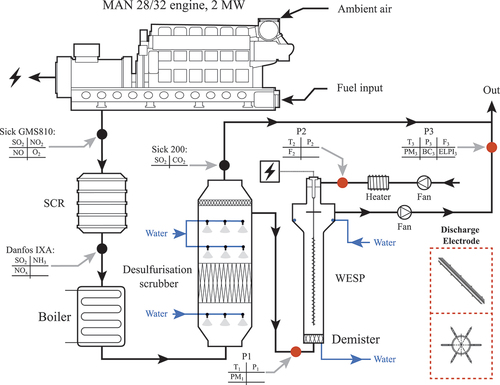
Figure 1. Schematic of the experimental setup. Three measurement points are marked with red spots and three gas measurement points are marked with black spots. During the experiments the temperature, T, pressure, P, and gas flow volume, F, were measured.

The electrode used during the experiment is shown in the southeast corner.

High discharge current, I, operation Voltage, V, current density, J, and particle residence time, t_pr, are the key operating parameters for the removal efficiency of a WESP. A high level of current-voltage increases particle saturation charge, q_s, which in combination with a raised voltage provides an increase in particle migration velocity, ω, from the discharge electrode to the collection electrode. An increased migration velocity decreases the time needed for a particle to migrate to the collection electrode; however, a specific particle residence time is still needed in order for different particle sizes to be charged, accelerated, and moved to the collection electrodes, which emphasizes the importance of the particle residence time for increasing the removal efficiency (Sadeghpour et al. 2021). WESPs are mainly cylindrical/hexagonal systems, based on the shape of their collection electrodes, where the collection electrode is continuously cleaned with a water film (Yang et al. 2017; Zheng et al. 2018). Yang et al. (2017) tested two different spike electrode designs where a fishbone configuration achieved the highest level of current density. The study also investigates the effect of particle residence time on removal efficiency, for different particle sizes, in the range from ≈1–2 s showing enhanced removal rates with increased particle residence time. Zheng et al. (2018) tested different discharge electrode configurations in a hexagonal column with different spike lengths, spacing, and rotation angles. Longer spikes with a shorter spacing increased the current density output, while the rotation angle showed the highest removal efficiency when pointing to the corners. Wang et al. (2019) used the results from Zheng et al. (2018) to investigate the ionic winds generated in the WESP numerically using spikes with a length of ≈15 mm from the discharge electrodes body, the tube part of the electrode. The study showed ionic winds going from the discharge electrode to the outer part of the collection electrodes. For industrial land-based applications, spiked discharge electrodes with hexagonal collection electrodes and with continuous cleaning are generally used for WESPs. As additional water consumption on board, a vessel increases the price due to electricity uses for pumping and water cleaning, it is relevant to investigate a WESP system with sequential cleaning for a marine application.

A WESP system with sequential cleaning for a marine application has never been investigated, and no work has been conducted to investigate the influence of small values of particle residence time (<1 s) on the removal efficiency of BC particles and different particle sizes. The influence of particle residence time is especially important for marine WESP systems, where space is limited, as it can be closely linked to the overall system size.

In this study, a full-scale hexagonal WESP column with sequential cleaning was experimentally tested using exhaust gas from a ≈2 MW marine diesel engine running on Heavy Fuel Oil (HFO) followed by a line of maritime exhaust gas cleaning treatment systems. The WESP column was operated at different particle residence time values, with a focus on the range from 0.35 to 0.95 s, and current–voltage inputs, in the form of electrical energy density, to investigate their influence on removal efficiencies of BC, PM, and different particle sizes. This provides knowledge to help predict the removal efficiencies of BC, PM, and different particles under different particle residence time, current, and voltage values.

System setup and experimental methods

A schematic diagram of the experimental setup is illustrated in Figure 1. The system mainly consists of five components: (1) an ≈2 MW marine engine, (2) a Selective Catalytic Reduction (SCR) module, (3) an exhaust gas boiler, (4) a desulfurization scrubber, and (5) a WESP. Parts 1–4 were held and operated with constant parameters during the experiments.

Constant system setup

To generate PM and BC particles for the experimental WESP setup a fourstroke marine engine, with a maximum power output of ≈2 MW operated at a constant engine load. The engine was fueled with HFO with a density of 0.9894 g/ml (15°C), sulfur level of 2.45%, and viscosity of 408.1 mm²/s (15°C). Before the exhaust gas reaches the WESP system, it passes through an SCR module where NO_x is removed, an exhaust gas boiler where the gas is cooled to exploit the heat, and a desulfurization scrubber where SO_x is removed. When passing through the scrubber, the exhaust gas is cooled to 30°C and relative humidity of 100% is achieved. After the scrubber, a portion of the flue gas, ranging from 5% to 10%, is redirected to the WESP system where a demister is located. The purpose of the demister is to remove water droplets and generate a uniform gas flow going into the WESP column. The operational parameters of the above-described system are held constant to ensure a stable PM and BC input of ≈130 and ≈19 mg/Nm³ to the WESP system, respectively.

Experimental WESP setup

The WESP system consists of a single hexagonal collection electrode and a negative DC discharge rod-electrode. The hexagonal collection tube, used as collection electrode, was installed vertically with a side length of ≈170 mm, a material thickness of 3 mm, and a vertical height of 4000 mm. The discharge electrode was a spike-electrode with a tube diameter of ≈30 mm, a spike height of 15 mm, spike spacing of 100 mm, and a maximum rated length of 2700 mm. The electrode was made out of three pieces of 900 mm in length. The discharge electrode was positioned in a manner where the spikes were pointing to the six corners of the hexagonal tube. The discharge electrode can be seen in the bottom right corner of Figure 1. An adjustable DC voltage from 0 to 76 kV was supplied to the discharge electrode during the experiments.

Measurement overview

During the experiments, the particle size distribution and BC particles were only measured after the WESP system. Instead of measuring before the WESP, it was assumed that measurements before and after the system were identical when the WESP was turned off. To verify this assumption, a series of BC measurements were performed before and after the WESP that showed a high level of consistency, thus verifying the assumption. PM measurements were made before and after the WESP system to generate a coherent data set to minimize possible fluctuations in the system.

The measurement points used during the tests can be seen as red marks in Figure 1; P1 and P3 illustrate the measurement points before and after the WESP, respectively. P2 was used to measure the flow, temperature, and pressure of the flushing air stream, which was used to keep the insulator box clean from particles. The PM mass was measured by gravimetric sampling on a planar filter according to EN13284-1 over a time interval of 600 s. The filters were dried and weighed before and after the PM measurement.

The particle size distribution was measured with an electrical low-pressure impactor (ELPI) from Dekati using a dilution ratio of 96, a particle density of 1460 kg/m³ (Corbin et al. 2018), and an output frequency of 5 s. As the particle density is higher than 1 kg/m³, the Stokes particle diameter, d_st,p, has been chosen as the output. Particle diameter will be used instead of Stokes particle diameter from this point onwards. The ELPI data were separated into 12 impactor stages with their corresponding Stokes particle diameter as seen in Table 1.

Table 1. Stokes particle diameter intervals and geometric mean Stokes particle diameters.

Impactor stage No. [−]	Stokes diam. range [μm]	Geom. Mean stokes diam. [μm]
1	0.005–0.020	0.01
2	0.020–0.039	0.03
3	0.039–0.068	0.05
4	0.068–0.117	0.09
5	0.117–0.203	0.15
6	0.203–0.302	0.25
7	0.302–0.493	0.39
8	0.493–0.769	0.62
9	0.769–1.302	1.00
10	1.302–1.956	1.60
11	1.956–3.280	2.53
12	3.280–8.171	5.18

The BC measurements were made with an AVL 415SE smoke meter (FSN).

Measurements were sampled at a frequency of ≈30 s and a length of ≈15 s. The length of the measurement varied with the particle load in the gas, where lower loads increase the measurement time. Before every BC measurement, the system is flushed with fresh air to remove deposited material.

The gas composition was measured at three different points: immediately after the engine, after the SCR system, and after the desulfurization scrubber. The three positions and their measurement components are marked with black marks in Figure 1. An O₂ and CO₂ measurement was also measured in parallel with the ELPI measurements.

Experimental approach

Different parameters such as electrode length, particle residence time, and current-voltage were varied with a focus on the difference in trapping efficiencies as a function of PM, BC, and different particle diameters.

Before starting a measurement, the electrode and collection electrode were flushed with water to remove any accumulated PM/BC particle coating that could affect the measurements.

At the start of the measurement campaign, the spark voltage was determined, which is a measure of the voltage at which continuous sparking occurs. A spark can be seen in the data as a sharp drop in the current–voltage data, which originates from a short circuit in the electrical system. To minimize sparking during the measurements, a maximum voltage was chosen by lowering the input to an acceptable level well below the spark voltage where few to no sparks occurred. For experiments with particles, an input of 72 kV was used. During the experiment, the voltage was held constant and the discharge current was detected after the corona onset. The voltage and discharge current were recorded every 2 s.

Data processing

The measurements were processed in four steps as depicted in Figure 2.

Figure 2. Description of the data processing steps for BC, ELPI, and PM.

The data processing was split into two routines: one for the BC/ELPI data and another for the PM data. The BC/ELPI data went through the following steps:

(Step 1) Detect sparks in the measurements that can be seen as sudden drops where the current–voltage data go to zero.

(Step 2.1) Remove data within the time range of a spark ±3 s.

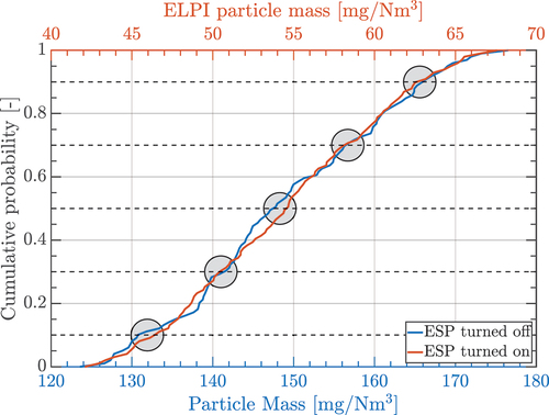
(Step 3.1) Plot the cumulative probability of the data with and without the WESP turned on. This part of the data processing focuses on fluctuations in the input data for the WESP system and how to calculate a reliable standard deviation for the ELPI and BC trapping efficiencies. The ELPI and BC data were greatly affected by fluctuations in the input data due to small sampling times of 5 and 15 s, respectively. In these cases, it was assumed that the fluctuations in the input exhaust gas data would correlate to the fluctuations measured after the WESP. Hence, to compare the two fluctuations, a cumulative distribution was made for the two data sets, an example of which can be seen in Figure 3.

Figure 3. Illustration of the cumulative probability for ELPI data when the WESP was turned on and off. Five comparison points, marked with a circle and a dashed line, are illustrated where removal efficiency and standard deviation are calculated.

(Step 4) calculate removal efficiency, with eq 4(4) $\eta \left(\mathrm{\%}\right)=\frac{{\dot{m}}_{off}{t}_{exp}-{\dot{m}}_{on}{t}_{exp}}{{\dot{m}}_{off}{t}_{exp}}\cdot 100\mathrm{\%}$(4) , and its standard deviation. This was achieved by comparing the two cumulative distributions at 100 evenly distributed lines and calculating a trapping efficiency at every line. A mean and a standard deviation were then generated from the values calculated at the 100 lines. On Figure 3, five dashed lines, intersecting with a circle, are drawn to illustrate the process.

The four steps for the PM data processing are described below:

(Step 1) Detect sparks in the measurements that can be seen as sudden drops where the current–voltage data go to zero. The same procedure as previously mentioned.

(Step 2.2) Calculate the extra accumulated mass on the PM filters from when the WESP system was down/not working as a function of a spark. The added mass per spark can be calculated with eq 1(1) $\begin{array}{rl}& m_{s,i}=\underset{\hspace{0.17em}}{\underset{Accumulatedmass}{\underbrace{\left({\dot{m}}_{off,i}-{\dot{m}}_{on,i}\right)\left(t_{s,end}-t_{s,0}\right)}}}\\ & \cdot \underset{Correctionterm}{\underbrace{\left(1-\frac{1}{t_{s,end}-t_{s,0}}\underset{t_{s,0}}{\overset{t_{s,end}}{\int }}\frac{I\left(t\right)}{I_{ref}}dt\right)}}\end{array}$(1) .

(1) $\begin{array}{rl}& m_{s,i}=\underset{\hspace{0.17em}}{\underset{Accumulatedmass}{\underbrace{\left({\dot{m}}_{off,i}-{\dot{m}}_{on,i}\right)\left(t_{s,end}-t_{s,0}\right)}}}\\ & \cdot \underset{Correctionterm}{\underbrace{\left(1-\frac{1}{t_{s,end}-t_{s,0}}\underset{t_{s,0}}{\overset{t_{s,end}}{\int }}\frac{I\left(t\right)}{I_{ref}}dt\right)}}\end{array}$(1)

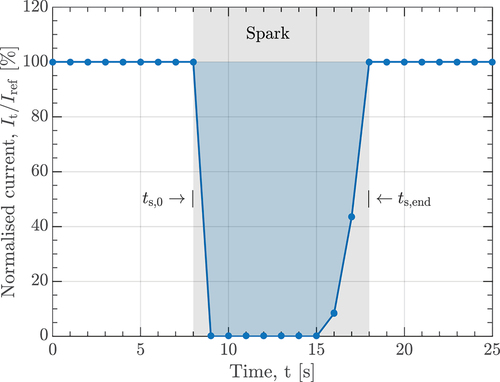
Where m_s,i is the added mass from a spark (mg), ˙m_off,i is added mass when the WESP is turned off (mg/s), ˙m_on,i is added mass when the WESP is turned on (mg/s), t_s,0 is the time at the start of a spark (s), t_s,end is the time at the end of a spark (s), I_t is the current during a spark (A), and I_ref is the average current before and after a spark (A). The average I_t/I_ref values during a number of sparks can be seen in Figure 4.

Figure 4. Illustration of normalized current, I_t/I_ref, as a function of time, t, where a spark can be seen in the gray/blue area.

(Step 3.2) Remove the added mass deposited on the filters from sparks. This can be done by multiplying m_s,i with the number of sparks during a measurement, as seen in eq 2(2) $m_a=m_{s,i}{n}_s$(2) .

(2) $m_a=m_{s,i}{n}_s$(2)

Where m_a is the total added mass to the filters (mg) and n_s is no. of sparks (-).

(Step 4) Calculate the removal efficiency and standard deviation. The removal efficiency was calculated with eq 3(3) $\eta \left(\mathrm{\%}\right)=\frac{{\dot{m}}_{off}\left(t_{exp}-t_{s,t}\right)-\left(\left({\dot{m}}_{on}{t}_{exp}-m_a\right)\left(t_{exp}-t_{s,t}\right)\right)}{{\dot{m}}_{off}\left(t_{exp}-t_{s,t}\right)}\cdot 100\mathrm{\%}$(3) for PM.

(3) $\eta \left(\mathrm{\%}\right)=\frac{{\dot{m}}_{off}\left(t_{exp}-t_{s,t}\right)-\left(\left({\dot{m}}_{on}{t}_{exp}-m_a\right)\left(t_{exp}-t_{s,t}\right)\right)}{{\dot{m}}_{off}\left(t_{exp}-t_{s,t}\right)}\cdot 100\mathrm{\%}$(3)

where η is the removal efficiency (%), t_exp is the time of the measurement (s), and t_s,t is the total time of sparks during a measurement (s). Equation 3(3) $\eta \left(\mathrm{\%}\right)=\frac{{\dot{m}}_{off}\left(t_{exp}-t_{s,t}\right)-\left(\left({\dot{m}}_{on}{t}_{exp}-m_a\right)\left(t_{exp}-t_{s,t}\right)\right)}{{\dot{m}}_{off}\left(t_{exp}-t_{s,t}\right)}\cdot 100\mathrm{\%}$(3) is reduced to eq 4(4) $\eta \left(\mathrm{\%}\right)=\frac{{\dot{m}}_{off}{t}_{exp}-{\dot{m}}_{on}{t}_{exp}}{{\dot{m}}_{off}{t}_{exp}}\cdot 100\mathrm{\%}$(4) to calculate the removal efficiency for the BC and ELPI data.

(4) $\eta \left(\mathrm{\%}\right)=\frac{{\dot{m}}_{off}{t}_{exp}-{\dot{m}}_{on}{t}_{exp}}{{\dot{m}}_{off}{t}_{exp}}\cdot 100\mathrm{\%}$(4)

Results and discussion

Effect of electrode lengths and general size distribution

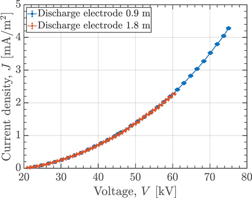
To be able to compare data from different discharge electrodes, it is important that different lengths generate the same current density at similar voltage inputs. This has been investigated in Figure 5, which shows the current density as a function of voltage, with two discharge electrode lengths of 0.9 and 1.8 m. The average current density, J, in Figure 5 is based on the current density distribution on the collecting electrodes that had an average area of 1.03 m² per meter of electrode. Figure 5 shows a similar tendency for the two electrode lengths when increasing the input voltage and the calculated standard deviations only show minor variations giving the overall tendencies. It can be seen that the current density for the 0.9 m electrode can be increased to a higher level compared with the 1.8 m electrode, which is due to the cap of 4.5 mA for the high voltage power supply. The comparability of the two voltage and current density curves verifies the possibility to compare measurements from different electrode lengths.

Figure 5. Effect of different discharge electrode lengths as a function of current density, J, and voltage, V.

During the experiments, the particle distribution input to the WESP system where kept as constant as possible with an average PM input of ≈130 mg/Nm³ and BC input of ≈19 mg/Nm³. The particle distribution and fluctuations can be seen in Figure 6.

Figure 6. Particle diameter, d_st,p, mass distribution of the gas input for the WESP and their standard deviation.

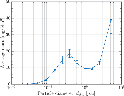
The size distribution of the gas input in Figure 6 has been generated from a series of ELPI measurements generated after the WESP column when the system was turned off.

The first impactor stage (0.005–0.020 µm) has been removed from the data series as the measurements showed long periods without any particles in this range. The standard deviations shown in Figure 6 show large fluctuations for particles with a mean diameter of 5.18 µm with a deviation of 8.3%. The remaining particle diameters showed relatively small deviations compared to 5.18 µm.

Particle residence time and size

The influence of particle residence time, t_pr, and particle diameter, d_st,p, on the trapping efficiency has been investigated with ELPI particle diameter data. The evaluation was made at a constant voltage input of 72 kV where the residence time was varied by changing the discharge electrode length and gas velocity. Particle residence times ranging from 0.3 to 0.43 s were performed with an electrode length of 0.9 m, and the rest were performed with a length of 1.8 m.

Figure 7 displays the trapping efficiency for two-particle ranges (0.02–1.30 µm and 1.30–8.17 µm) and the overall particle range (0.02–8.17 µm). The mass contained in the two-particle ranges corresponds to 48% and 52% of the total mass. In Figure 7 particle diameters between 1.30 and 8.17 µm shows a decreased removal efficiency compared to the overall (0.02–8.17 µm) at a particle residence time of 0.3 s, where particle diameters between 0.02 and 1.30 µm show an increased removal efficiency. This gap in removal efficiency is minimized as the particle residence time goes from 0.3 to 0.95 s where 0.02–8.17 µm increased by 31.7%, 0.02–1.30 µm with 29.4%, and 10–12 with 34.1%. For further insight into the removal efficiency of different particle sizes, Figure 7 is divided into its full range of sizes at their corresponding particle residence times, as seen in Figure 8.

Figure 7. Trapping efficiencies at different particle residence times, t_pr, for particle diameters between 0.02–1.30 µm, 1.30–8.17 µm, the overall range 0.02–8.17 µm, with their percentage of the total mass, m_t, and depicted with standard deviations.

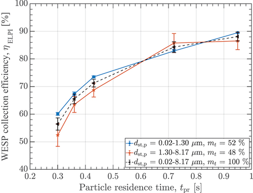
Figure 8. Removal efficiencies for different mean stokes diameters, d_st,p at various particle residence times, t_pr.

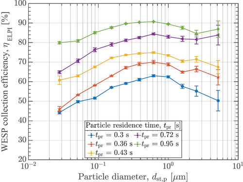
Figure 8 describes a tendency where particles with a diameter between 0.02 and 0.2 µm and 1.30–8.17 µm fall behind in the removal efficiency compared to 0.20–1.30 µm; especially, at small particle residence times. The variations in removal efficiency between different particle sizes decrease as the particle residence time increases toward 0.95 s. These changes in removal variations give an insight into the removal rates for different sizes, highlighting the importance of knowing the particle residence time and the particle size distribution.

Figure 8 illustrates variations of up to 24.1% between different particle diameters. Particles with a diameter of 0.03 µm measured the smallest average removal efficiency, which on average was 14.0% lower than the average overall trapping efficiency, which can be found in Figure 8. Particles with a diameter of 0.62 µm showed the largest average removal efficiency which on average was 3.4% higher than the overall trapping efficiency. The three largest particle diameters (1.308.17 µm) had a decreased removal efficiency of 8.7% at a residence time of 0.3 s compared to particles with a mean diameter of 0.62 µm. This decrease in removal efficiency was reduced to 5.5% at a residence time of 0.36 s and further reduced to 4.3% at a residence time of 0.95 s. This phenomenon may occur due to longer charging times for larger particles, but also a slower acceleration before the particles reaches the maximum migration velocity. The charging time is further increased at low particle residence times due to a large amount of space charge, as an effect of large amounts of particles in the start, which is quickly reduced as more than 50% of the particles are removed/trapped in the first 0.3 s.

The particles with the smallest diameter (0.02–0.2 µm) also start with a decreased removal efficiency of 14.5% at a residence time of 0.3 s compared to particles with a diameter of 0.62 µm. The decrease in removal efficiency was reduced to 8.7% at a residence time of 0.95 s. For these diameters, the particles charging time is decreased as described by the charging equations created by (Lawless 1996). The acceleration is also increased due to the reduced slip when approaching the molecular mean free path which is ≈69 nm (30°C, 1 atm, and relative humidity 100%); however, the maximum migration velocity also decreases as a function of the particle diameter increasing the time needed to travel to the collection electrodes. Another way to collect the particles between 0.02 and 0.2 µm is by generating ionic winds, which is the gas flow induced by electrostatic forces and is mainly linked to the corona discharge from the discharge electrode that forces the gas stream toward the collection electrodes that also carries the particles with it (Dau et al. 2018; Wang et al. 2019; Zheng et al. 2018). Nevertheless, the ionic winds are greatly reduced as a function of the large amount of space charge at small particle residence times. The amount of space charge decreases with particle residence time as the number of particles in the system is reduced, which may be a major factor for the decreased removal efficiency for particles ranging from 0.02 to 0.2 µm.

Effect of electrical energy density and particle residence time

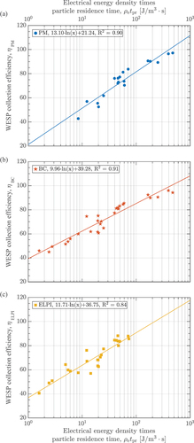
The effect of the electrical energy density, ρ_e, reference to the amount of J transferred to one m³ of gas going through the WESP system. It can be calculated by taking the current density and dividing it with the gas velocity times the WESP inlet area. It can be calculated with the following. The effect of electrical energy density was investigated by changing the voltage input to the system, which can be seen in Figure 9. Between Figure 9a,b the particle residence time was doubled which increased the trapping of larger particles, fitting well with the results and knowledge discussed in section 3.2. In general, the data showed a similar increase in removal efficiency over the whole range of particle sizes when the electrical energy density was raised. By combining the effect of electrical energy density and the particle residence time (investigated in Section 3.2) a general trapping efficiency as a function of electrical energy density and particle residence time can be generated as seen in Figure 10. A logarithmic x-axis is used for the plot to increase the visibility of the data. The three measurement methods show a growing trapping efficiency with the combined value of electrical energy density, ρ_e, and particle residence time, t_pr. The removal efficiency for PM increased from 42.7% to 97.2%, BC from 44.8% to 95.9%, and ELPI measurements from 40.5% to 88.2%. The main difference between the three methods is at the start of the graph, where the PM measurement starts ≈20% lower than the BC and ELPI data. The PM trapping catches up to the BC Data when approaching 100%. The PM and BC trends reach 100% at 408.4 and 444.3 J/m³·s, respectively. This corresponds to an 8.8% value increase for the BC trend compared to the PM trend. The ELPI trend reached 100% at 221.71 J/m³·s which corresponds to a decrease of 45.7% and 50.1% compared to the PM and BC trends, respectively. The ELPI trend should; however, not be used for removal efficiencies above ≈88% as ELPI data were absent for these levels.

Figure 9. WESP mass trapping efficiency, measured with ELPI, for different electrical energy densities with a constant particle residence time, t_pr, of 0.36 s for (a) and 0.72 s for (b).

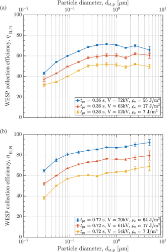
Figure 10. Trapping efficiency of PM (a), BC (b), and ELPI (c) as a function of electric energy density, ρ_e, times the particle residence time, t_pr.

BC removal efficiency compared to total PM and different particle diameter sizes

The following section describes the variations between the three measurement methods used in this study, where the measured BC data were compared to the PM and ELPI data. The BC data were chosen as the main data source as it had the highest number of synchronized data points with the PM and ELPI data. Figure 11 displays the variations between the measured BC and PM data.

Figure 11. Comparison between PM and BC collection efficiencies, η.

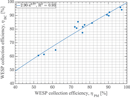
The PM trapping efficiency starts ≈7% lower than the corresponding BC data, after which the gap decreased as the efficiency rose toward 100%. Figure 12 displays the comparison between the BC and ELPI trapping efficiencies. (A) illustrates the scatter plot of the total ELPI data (0.02–8.17 µm) and BC. It can be seen that the two measurement methods follow a similar tendency despite the BC data starting ≈4% higher than the ELPI data and ends ≈1% lower. The shift between the PM/ELPI data to the BC data may be explained with the particle range of agglomerated BC particles where primary BC particles have been measured to ≈40 nm (Choi et al. 2019; Clague et al. 1999; Mikhailov et al. 2006; Xi and Zhong 2006).

Figure 12. Comparison between ELPI and BC collection efficiencies, η, scatter plot with ELPI data from 0.02–8.17 µm and from 0.02–0.49 µm.

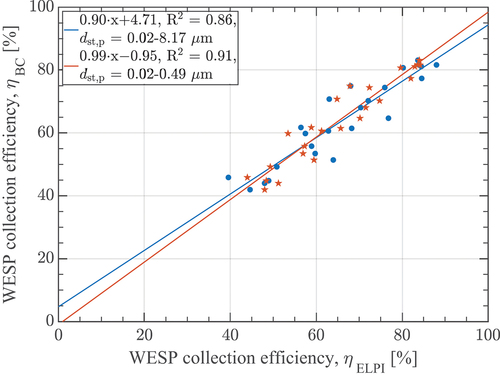
To investigate the range of agglomerated BC particles, the different ranges of ELPI bins have been compared to the BC data. It was found that ELPI measurements for particles ranging from 0.02 to 0.49 µm generated the best coherent data comparison with the BC data. When changing the ELPI particle diameter range from 0.02–8.17 µm to 0.02–0.49 µm the trendline set point on the y-axis decreased from 3.74 to 0.06 and the slope increased from 0.92 to 0.97. Thereby, increasing the similarity between the two measurement methods. The new trend line can be seen in red in Figure 12 showing the comparison between particles with a diameter between 0.02 and 0.49 µm and the BC data, illustrating an almost perfect fit between the two measurement methods. The range of agglomerated BC particles also explains the difference between the BC and PM data in Figure 11, where the BC data measures ≈7% higher than the PM at small particle residence times, which were decreased to ≈ 0% when going toward 100

% removal efficiency. This change can be found from ELPI diameters ranging from 0.49 to 8.17 µm, which is not comprised in the BC data, as the largest particles need appropriate time for their charging and acceleration process to become trapped.

Conclusion

This study made an experimental evaluation of a hexagonal wet electrostatic precipitator systems ability to clean exhaust gas, generated by a marine diesel system operating on heavy fuel oil. The study investigates the removal efficiency of different particle sizes, total particulate matter, and black carbon particles under different particle residence times, discharge currents, and voltages. The main conclusions from the study are as follows:

1. The wet electrostatic precipitator system was able to remove from 42.7% to 97.2% of the particulate matter and 44.8% to 95.9% of black carbon particles by varying the electrical energy input to the gas stream and the particle residence time, which is illustrating a large flexibility of the wet electrostatic precipitator system.

2. The particle removal efficiencies were largely affected by the size of the particles, which generated variations of up to 24.1%. Particles with a mean diameter of 0.03 µm measured the smallest average removal efficiency, which was 14.0% lower than the average overall trapping efficiency. Particles with a mean diameter of 0.62 µm showed the largest average removal efficiency which on average was 3.4% higher than the overall trapping efficiency.

3. Particle residence times in the wet electrostatic precipitator system had a large effect on the trapping efficiency, showing an overall increase of 31.7% when increasing the time from 0.3 to 0.95 s. The largest increase was observed for particles with a mean size of 5.18 µm where the removal efficiency was increased by 36.7%. Particles with a mean size of 5.18 µm started with a removal efficiency that was 6.2% lower at 0.3 s, compared to the overall removal efficiency, which decreased to 1.2% at 0.95 s. Hence, particles with a mean size of 5.18 µm needed a longer particle residence time due to a longer charging and acceleration time.

4. It was found that the best fit between the ELPI and black carbon data was with an ELPI particle size range between 0.02 and 0.49 µm, which changed the trend line between the measurements from 0.92x + 3.74 to 0.97x + 0.06 making an almost perfect fit between the two, indicating a black carbon range between 0.02 and 0.49 µm.

5. The study indicates that a similar removal efficiency between black carbon and particulate matter could be achieved and that the main focus for improvement of black carbon removal should be found in the particle range of 0.02–0.49 µm.

Acknowledgement

The authors would like to thank Christian Andersson for his contribution in the fabrication of the experimental setup.

Disclosure statement

No potential conflict of interest was reported by the author(s).

Data availability statement

Raw data were generated at Alfa Lavals test center, Aalborg. Derived data supporting the findings of this study are available from the corresponding author NHH on request.

Additional information

Funding

This work is financially supported by the Danish Innovation Foundation under grant no. 8053-00172B.

Notes on contributors

Nick Høy Hansen

Nick Høy Hansen is a Ph.D. candidate at the department of Energy, Aalborg University, with a research focus on wet electrostatic precipitation.

Henrik Sørensen

Henrik Sørensen is Associate Professor and Head of section for Thermal Engineering at the Department of Energy, Aalborg University, Denmark.

Jakob Hærvig

Jakob Hærvig is an associate professor at AAU Energy, Aalborg University.

References

- AMAP, Arctic Climate Change Update. 2021. Key trends and impacts. Summary for Policy-Makers — AMAP, Technical Report. Arctic Monitoring and Assessment Programme. https://www.amap.no/documents/doc/arctic-climate-change-update-2021-key-trends-and-impacts.-summary-for-policy-makers/3508.
- Beltran, M. R. 2009. Wet ESP for the collection of submicron particles, mist and air toxics.
- Choi, J. H., D. Y. Kim, W. J. Lee, and J. Kang. 2019. Conversion of black carbon emitted from diesel-powered merchant ships to novel conductive carbon black as anodic material for lithium ion batteries. Nanomaterials 9 (9):1280. doi:10.3390/nano9091280.
- Clague, A. D., J. B. Donnet, T. K. Wang, and J. C. Peng. 1999. A comparison of diesel engine soot with carbon black. Carbon 37:1553–65.
- Corbin, J. C., S. M. Pieber, H. Czech, M. Zanatta, G. Jakobi, D. Massab`o, J. Orasche, I. El Haddad, A. A. Mensah, B. Stengel, et al. 2018. Brown and black carbon emitted by a marine engine operated on heavy fuel oil and distillate fuels: Optical properties, size distributions, and emission factors. J. Geophys. Res. Atmos. 123 (11):6175–95. doi:10.1029/2017JD027818.
- Dau, V. T., T. X. Dinh, C. D. Tran, T. Terebessy, T. C. Duc, and T. T. Bui. 2018. Particle precipitation by bipolar corona discharge ion winds. J. Aerosol. Sci. 124:83–94.
- Dou, T. F., and C. D. Xiao. 2016. An overview of black carbon deposition and its radiative forcing over the arctic. Adv. Clim. Chang. Res. 7:115–22.
- Ehara, Y., A. Osako, A. Zukeran, K. Kawakami, and T. Inui. 2014. Diesel PM collection for marine emission using hole-type electrostatic precipitators. WIT Trans. Ecol. Environ. 183:145–55.
- Flanner, M. G., C. S. Zender, J. T. Randerson, and P. J. Rasch. 2007. Present day climate forcing and response from black carbon in snow. J. Geophys. Res. Atmos. 112 (D11):11202. doi:10.1029/2006JD008003.
- Gagn´e, S., M. Couillard, Z. Gajdosechova, A. Momenimovahed, G. Smallwood, Z. Mester, K. Thomson, P. Lobo, and J. C. Corbin. 2021. Ash-decorated and ash-painted soot from residual and distillate-fuel combustion in four marine engines and one aviation engine. Environ. Sci. Technol. 55 (10):6593. doi:10.1021/acs.est.0c07130.
- Hansen, H. N., S. K. Jensen, S. Gagn´e, S. Molgaard, F. Bak. 2018. PPR 6/INF.13, evaluation of the effect of SCR, EGC and sulphur limit solutions on black carbon emissions from ships using three black carbon measurement methods. Canada & Denmark submission. Technical Report. Sub-Committee on Pollution Prevention and Response.
- IMO. 2020. Fourth IMO GHG study 2020 full report. Technical Report. International Maritime Organization.
- Jaworek, A., A. Krupa, and T. Czech. 2007. Modern electrostatic devices and methods for exhaust gas cleaning: A brief review. J. Electrost. 65:133–55.
- Lawless, P. A. 1996. Particle charging bounds, symmetry relations, and an analytic charging rate model for the continuum regime. Technical Report 2.
- Lin, G. Y., C. J. Tsai, S. C. Chen, T. M. Chen, and S. N. Li. 2010. An efficient single stage wet electrostatic precipitator for fine and nanosized particle control. Aerosol Sci. Technol. 44 (1):38–45. doi:10.1080/02786820903338298.
- MEPC. 2011. Report of the marine environment protection committee on its sixty-second session, MEPC 62/24. Technical Report. Marine Environment Protection Committee.
- Mikhailov, E. F., S. S. Vlasenko, I. A. Podgorny, V. Ramanathan, C. E. Corrigan, A. Remsen, D. A. Dieterle, K. L. Carder, F. R. Chen, G. A. Vargo, et al. 2006. Optical properties of soot-water drop agglomerates: An experimental study. J. Geophys. Res. Atmos. 111 (C11003):111. doi:10.1029/2004JC002813.
- Sadeghpour, A., F. Oroumiyeh, Y. Zhu, D. D. Ko, H. Ji, A. L. Bertozzi, and Y. S. Ju. 2021. Experimental study of a string-based counterflow wet electrostatic precipitator for collection of fine and ultrafine particles. J. Air Waste Manag. Assoc. 71 (7):851–65. doi:10.1080/10962247.2020.1869627.
- Sapra, H., M. Godjevac, K. Visser, D. Stapersma, and C. Dijkstra. 2017. Experimental and simulation-based investigations of marine diesel engine performance against static back pressure. Appl. Energy 204:78–92.
- Shindell, D., and G. Faluvegi. 2009. Climate response to regional radiative forcing during the twentieth century. Nat. Geosci. 2 (4):294–300. doi:10.1038/ngeo473.
- Sofiev, M., J. J. Winebrake, L. Johansson, E. W. Carr, M. Prank, J. Soares, J. Vira, R. Kouznetsov, J. P. Jalkanen, J. J. Corbett. 2018. Cleaner fuels for ships provide public health benefits with climate tradeoffs. Nat Commun. 9 (1): 1–12.
- Wang, X., J. Chang, C. Xu, J. Zhang, P. Wang, and C. Ma. 2016. Collection and charging characteristics of particles in an electrostatic precipitator with a wet membrane collecting electrode. J. Electrost. 83:28–34.
- Wang, Y., W. Gao, H. Zhang, C. Huang, K. Luo, C. Zheng, and X. Gao. 2019. Insights into the role of ionic wind in honeycomb electrostatic precipitators. J. Aerosol. Sci. 133:83–95.
- Wang, X., and C. You. 2013. Effects of thermophoresis, vapor, and water film on particle removal of electrostatic precipitator. J. Aerosol. Sci. 63:1–9.
- Xi, J., and B. J. Zhong. 2006. Soot in diesel combustion systems. 10.1002/ceat.200600016.
- Yang, Z., C. Zheng, Q. Chang, Y. Wan, Y. Wang, X. Gao, and K. Cen. 2017. Fine particle migration and collection in a wet electrostatic precipitator. J. Air Waste Manage. Assoc. 67:498–506.
- Zhang, H. D., Y. X. Zhou, and H. Long. 2015. Study on application conditions of wet electrostatic precipitators in coal-fire power plants. Electr. Power 48:13–16.
- Zheng, C., Y. Wang, X. Zhang, Z. Yang, S. Liu, Y. Guo, Y. Zhang, Y. Wang, and X. Gao. 2018. Current density distribution and optimization of the collection electrodes of a honeycomb wet electrostatic precipitator. RSC Adv. 8:30701–11.