Assessment of progress toward regional haze rule visibility goals using United States anthropogenic emissions rate of progress

ABSTRACT

The U.S. EPA developed the Regional Haze Rule to address Section 7491 of the 1977 Clean Air Act Amendments to prevent any future and remedy any existing visibility impairment due to manmade air pollution at Federal Class I areas (CIAs). The rule addresses this national goal by requiring states to show they are making progress toward estimated natural conditions by 2064 for the 20% anthropogenically Most Impaired Days (MID). For the MID, days that have high haze contributions from wildfires and windblown dust tend to be excluded using haze contributions from Carbon and crustal material as surrogates. To show progress toward natural conditions in 2064, a Uniform Rate of Progress Glidepath is defined as a straight line from measured 2000–2004 IMPROVE MID Baseline to natural conditions in 2064. Photochemical modeling is used to project the observed IMPROVE 2014–2018 MID visibility to 2028 that is compared to the Glidepath at 2028 to determine whether the MID visibility at a CIA is on a path toward natural visibility conditions in 2064. This paper discusses an alternative approach for showing progress toward no manmade impairment by using modeling results to generate a U.S. Anthropogenic Emissions Rate of Progress (RoP). The CAMx photochemical grid model was run for a current year (representing 2014–2018), 2028 future year and a 2002 past year and source apportionment was used to isolate the contributions of U.S. anthropogenic emissions to PM concentrations and visibility extinction. A RoP slope line is drawn from the 2002 visibility extinction due to U.S. anthropogenic emissions to zero in 2064 and the CAMx 2028 visibility for U.S. anthropogenic emissions is compared with the RoP slope line at 2028 to determine whether visibility due to U.S. anthropogenic emissions is on a path toward no U.S. manmade impairment in 2064.

Implications: The U.S. EPA Regional Haze Rule guidance to show progress toward no U.S. manmade visibility impairment at Class I Areas by 2064 backs into the U.S. manmade impairment contribution by using total atmospheric haze based on measured PM concentrations and subtracting uncertain estimates of routine natural and episodic (i.e. wildfires and windblown dust) natural conditions. The guidance also recommends accounting for visibility contributions due to international anthropogenic and prescribed fire emissions that are also uncertain. This paper presents an alternative approach that models the contributions of U.S. anthropogenic emissions to visibility for past, current and future years using source apportionment to show that U.S. anthropogenic emissions visibility impairment at Class I areas are on a path toward no contribution in 2064. Many U.S. anthropogenic emissions (e.g. power plants with continuous emissions monitoring systems) are better known and characterized than international, fire and natural emissions so the alternative approach should provide a better assessment of whether U.S. anthropogenic emissions are on a path toward no manmade impairment in 2064 than using trends in the measured visibility most impaired days that rely on uncertain estimates of haze due to wildfire, windblown dust, and international emissions and uncertain estimates of natural conditions in 2064.

Introduction

Section 7491 of the 1977 Clean Air Act Amendments (CAAA) states “Congress hereby declares as a national goal the prevention of any future, and the remedying of any existing, impairment of visibility in mandatory class I Federal areas which impairment results from manmade air pollution” (CAAA, 1977). In response to this national goal, in 1999 the United States Environmental Protection Agency (U.S. EPA) developed the Regional Haze Rule (RHR; U.S. EPA, 1999) that was revised in January 2017 (U.S. EPA, 2017). Regional haze is defined as visibility impairment that is caused by the emission of air pollutants from numerous anthropogenic sources located over a wide geographic area (40 CFR 51.301). Haze in the atmosphere is caused by air pollutants that absorb or scatter light reducing visual range and causing a loss of color, contrast, and detail in visual landscapes (NRC, 1993). There are 156 Federal Class I areas (CIAs), which are national parks greater than 6,000 acres and wilderness areas greater than 5,000 acres in existence in August 1977, that are offered special visibility protection under the 1977 CAAA and RHR. The 1999 RHR requires states to develop regional haze State Implementation Plans (SIPs) every 10 years that demonstrate reasonable progress for improving visibility in CIAs. The goal of the RHR, as modified in January 2017 (U.S. EPA, 2017), is to improve visibility for the 20% most anthropogenically impaired days and have no degradation for the 20% clearest days. The RHR requires states to set a reasonable progress goal (RPG) for visibility improvement on the 20% most impaired days in the context of other RHR requirements to be addressed in each State’s Implementation Plan (RHR SIP) and compare the RPG to a uniform rate of progress (URP) calculated as the straight line Glidepath (in deciviews) from the observed visibility for the 2000–2004 baseline period to estimated natural visibility conditions 2064 end-point year. If a state’s RPG did not achieve the URP Glidepath, the state has to demonstrate why the URP was not reasonable and the state’s RPG was reasonable. The RHR SIPs for the second implementation period (2018–2028) address progress toward natural conditions in 2064 with an RPG for the milestone year 2028.

The Interagency Monitoring of Protected Visual Environments (IMPROVE; Solomon et al., 2014) monitoring network collects particulate matter (PM) observations that are used to calculate light extinction. Each CIA has an associated IMPROVE monitoring site that is used to represent visibility at the CIA. The IMPROVE PM species are converted from concentrations (µg/m³) to light extinction (in inverse megameters, Mm⁻¹) using the revised (second) IMPROVE extinction equation (Pitchford et al., 2007). The IMPROVE extinction equation converts measured fine particulate matter (PM_2.5) ammonium sulfate (AmmSO4), ammonium nitrate (AmmNO3), organic matter carbon (OMC), elemental carbon (EC) and crustal material (Soil) and coarse PM (PMC or PM_2.5-10) into light extinction, accounting for effects of relative humidity on hygroscopic species (e.g., AmmSO4 and AmmNO3).

U.S. EPA developed a new Most Impaired Days (MID) visibility metric at the time of the January 2017 RHR changes based on measured PM species concentrations at IMPROVE monitoring sites that is the recommended metric for tracking visibility progress toward natural conditions (U.S. EPA, 2018a). The EPA method for identifying the IMPROVE MID uses a statistical procedure that is designed to identify days at IMPROVE monitoring sites most likely to be impaired by anthropogenic emissions. Using the IMPROVE sampling record from 2000 to 2014, the IMPROVE MID statistical procedure estimates the contributions of routine natural haze, which includes some AmmSO4 and AmmNO3, and natural haze due to episodic events using measured light extinction due to carbon and geogenic species as proxies for impacts due to, respectively, wildfires and windblown dust (WBD) with the remainder of the extinction assumed to be mainly anthropogenic in origin (less the routine natural conditions). This has an effect of measured extinction due to AmmSO4 and AmmNO3 being primarily from manmade emissions. The contribution of routine natural conditions is assumed to vary from day-to-day proportional to the total extinction for each species, after excluding the estimated contribution from natural episodic events. The IMPROVE MID visibility metric is obtained for each year as the 20% days with highest fraction of estimated anthropogenic visibility impairment after the statistical procedures have identified the natural components due to fire and dust contributions that are inferred from, respectively, carbon and geogenic filter mass measurements and routine natural background. The IMPROVE MID is the metric recommended by EPA to evaluate progress for the 2028 planning milestone toward reaching the distant long-term goal of achieving estimated natural conditions at CIAs by 2064 (U.S. EPA, 2018a).

States use photochemical grid models on a regional basis to simulate current and future year emission scenarios, with the modeling results for the current year MID used to project the current year observed MID visibility to the future year RPG MID visibility. The projected 2028 RPG MID visibility is compared to the URP Glidepath at 2028 to demonstrate visibility benefits of anthropogenic emission reductions and determine if visibility impairment at the CIA is on a path to natural conditions in 2064 (i.e., 2028 MID projection on or below the URP Glidepath) and assess inter-jurisdictional emissions transport. If the modeled estimates of natural and anthropogenic pollutant contributions on the observed MID differ from the estimates used in the operational analysis of the IMPROVE data to define the MID, the two approaches could be inconsistent and estimate different rates of visibility improvements by 2028.

EPA guidance allows for adjusting the URP Glidepath to account for contributions from international anthropogenic emissions (“international emissions”) and/or wildland prescribed burns (“Rx fire”) “if the adjustment has been developed through scientifically valid data and methods” (U.S. EPA, 2018a). The URP Glidepath adjustment is made by adding the visibility contribution of international emissions and/or Rx fire, as calculated for the 2028 future year, to the natural conditions 2064 end-point. The slope of the adjusted Glidepath is less than the slope of the URP Glidepath. EPA guidance recommends using Chemical Transport Models (CTMs) to estimate the contributions of international and Rx fire emissions to visibility (U.S. EPA, 2018a).

In this paper, we present an alternative approach to EPA’s recommended URP Glidepath approach for demonstrating progress toward no impairment due to U.S. manmade emissions in 2064 using a modeled U.S. anthropogenic emissions Rate of Progress (RoP) analysis that compares the manmade visibility extinction in 2028 with an RoP slope from modeled manmade impairment in 2002 to zero manmade impairment in 2064. We also present a Dynamic Evaluation that evaluates the photochemical modeling system and projection procedure’s ability to estimate changes in visibility due to changes in emissions over time.

Methods

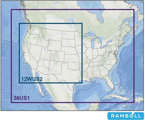
The Western Regional Air Partnership (WRAP; www.wrapair2.org) assisted western states in developing their RHR SIPs. WRAP developed a Technical Support System (TSS; https://views.cira.colostate.edu/tssv2/) that includes monitoring, emissions, modeling, and analysis products that states used as the technical basis for their RHR SIPs that were due to EPA by July 2021. WRAP developed a 2014 Photochemical Grid Model (PGM) modeling platform that was used to estimate 2028 visibility projections for the 20% MID that states used for their RPG and comparison with the URP and adjusted Glidepaths. The WRAP 2014 PGM modeling platform used an outer domain covering the U.S. and portions of Mexico and Canada with a 36-km grid resolution and a western U.S. domain with a 12-km grid resolution as shown in Figure 1 Version 7 of the Comprehensive Air-quality Model with extensions (CAMx; www.camx.com; Ramboll, 2020) PGM was used to model the 2014 calendar year using the 36/12-km domains with two-way grid nesting (i.e., pollutants flow freely back-and-forth between the 36-km and 12-km domains during the simulation). Meteorological inputs for the CAMx 2014 36/12-km modeling platform were based on a simulation of the Weather Research Forecast (WRF; Skamarock et al., 2008) meteorological model that was evaluated against calendar year 2014 meteorological measurements (Bowden, Talgo and Adelman, 2016). CAMx was first run for a 2014v2 base case emissions scenario that used actual emissions for the 2014 calendar year that was based on version 2 of the National Emissions Inventory (NEIv2; U.S. EPA, 2018b) with updates from western states in the U.S. (WRAP, 2019). The CAMx 2014v2 actual base case simulation was subjected to a model performance evaluation by comparing the modeled gaseous and particulate matter concentrations with concurrent observations. Model performance was documented on the WRAP TSS website (i.e., https://views.cira.colostate.edu/iwdw/docs/WRAP_WAQS_2014v2_MPE.aspx). The model was evaluated for total and species extinction at IMPROVE sites for four subregions in the western U.S. Although model performance frequently achieved model performance goals and criteria based on previous regional model applications (Emery et al. 2016), there were some species and specific areas with poorer model performance. For example, overestimates of sulfate in the Pacific Northwest and at western coastal sites, underestimates of nitrate on the Colorado Plateau, and poor model performance for PM from windblown dust. However, WRAP and the states determined that model performed well compared to previous applications and that the platform based on the 2014 calendar year was acceptable for use in simulating haze levels for typical emissions in 2014–2018 and emissions projections to 2028.

Figure 1. 36-km 36US1 and 12-km 12WUS2 modeling domains used in the WRAP 2014 modeling platform current (2014v2 and RepBase2) and future (2028otba2) year CAMx simulations for western states Regional Haze modeling.

WRAP conducted Representative Baseline (RepBase2) and 2028 On-the-Book (2028OTBa2) CAMx simulations as follows (WRAP, 2020a):

• RepBase2 emission scenario uses U.S. anthropogenic emissions representative of the 2014–2018 period, Representative Baseline open land fire emissions (RepBase Fire; Air Sciences, 2020) and 2014v2 natural emissions (e.g., biogenic, lightning NO_X and sea salt and dimethyl sulfide from oceans).

• 2028OTBa2 emissions scenario uses U.S. anthropogenic emissions representative of 2028 assuming current on-the-book controls with RepBase Fire and 2014v2 natural emissions.

For both the RepBase2 and 2028OTBa2 scenarios, international emissions from the EPA2016v1 modeling platform (U.S. EPA, 2021a) were used.

The CAMx Particulate Source Apportionment Technology (PSAT) particulate matter source apportionment tool (Ramboll, 2020; Vijayaraghavan et al., 2016; Koo et al., 2009) was used in both the RepBase2 and 2028OTBa2 CAMx simulations to separately track the contributions of U.S. anthropogenic emissions, international anthropogenic emissions, four types of open land fires (wildfires, wildland prescribed fires, and agricultural burning in the U.S. and non-U.S. fires), and natural emissions within the 36/12-km modeling domains. The PSAT source apportionment tool was also used to separately track Boundary Condition (BC) contributions through the 36-km domain boundaries due to natural sources, international anthropogenic emissions, and U.S. anthropogenic emissions (either from circling the globe or from wind flow changes causing recirculation). The CAMx 2014 modeling platform BCs were defined by running GEOS-Chem (v12.2.0) global chemistry model (Bey et al.,2001; Keller et al., 2014) for a 2014 base case and two 2014 zero-out emissions cases for international anthropogenic and U.S. anthropogenic emissions.

2028 visibility projections were made following EPA’s guidance (U.S. EPA, 2018c) that use the CAMx RepBase2 and 2028OTBa2 modeling results in a relative fashion to scale the observed IMPROVE concentrations from the 2014–2018 IMPROVE MID to 2028. The model derived species-specific scaling factors are called Relative Response Factors (RRFs) and are defined as the ratio of the average CAMx future (2028OTBa2) to average current (RepBase2) year modeling results where the average is across days in the 2014 IMPROVE MID. For example, the equations for SO4 concentrations from the 2014–2018 IMPROVE MID are as follows:

$\mathrm{R}\mathrm{R}{\mathrm{F}}_{\mathrm{S}\mathrm{O}4}=\sum 2028\mathrm{O}\mathrm{T}\mathrm{B}\mathrm{a}{2}_{\mathrm{S}\mathrm{O}4}/\sum \mathrm{R}\mathrm{e}\mathrm{p}\mathrm{B}\mathrm{a}\mathrm{s}\mathrm{e}{2}_{\mathrm{S}\mathrm{O}4}$

$\mathrm{P}\mathrm{r}\mathrm{o}\mathrm{j}\mathrm{e}\mathrm{c}\mathrm{t}\mathrm{e}\mathrm{d}\mathrm{\_}2028_{\mathrm{S}\mathrm{O}4}=\mathrm{I}\mathrm{M}\mathrm{P}\mathrm{R}\mathrm{O}\mathrm{V}\mathrm{E}\mathrm{\_}2014-2018_{\mathrm{S}\mathrm{O}4}\mathrm{x}\mathrm{R}\mathrm{R}{\mathrm{F}}_{\mathrm{S}\mathrm{O}4}$

Details on the EPA-recommended visibility projection approach are contained in their modeling guidance (U.S. EPA, 2018c). WRAP used three approaches for projecting 2028 visibility for the MID that differ in how days with modeled fire impacts are treated and which days are used to develop the RRFs. The three visibility projection procedures are as follows (WRAP, 2021):

EPA: The EPA default projection approach follows the procedures in EPA’s guidance (U.S. EPA, 2018c) to project the observed 2014–2018 IMPROVE MID using RRFs based on average modeled concentrations across days in the 2014 IMPROVE MID.

EPAwoF: Even though the IMPROVE MID are obtained using a statistical procedure that limits the influence of fires on IMPROVE concentrations for days in the MID, large, modeled fire impacts can still occur on the observed 2014 IMPROVE MID used in the EPA default projection method. The EPA without fire (EPAwoF) method uses the RepBase2 and 2028OTBa2 PSAT source apportionment results to remove the contributions of emissions from U.S. wildfires (WF), U.S. wildland prescribed burns (Rx fire), and non-U.S. (Mexico and Canada) fires from the, respectively, RepBase2 and 2028OTBa2 modeling results used in the RRFs. Thus, the EPAwoF method RRFs are based on the same days in the observed 2014 IMPROVE MID as used by the EPA default method, only the contributions from U.S. WF and Rx fire and non-U.S. fires have been removed in the calculation of the RRFs.

ModMID: The third method uses the modeled most impaired days (ModMID) to calculate the RRFs, but still applies the RRFs to the observed 2014–2018 IMPROVE MID. The days in the ModMID are defined as the 20% days with the highest fraction of impairment due to U.S. anthropogenic emissions (i.e., 20% highest Bext_USAnthro/Bext_Total days). As in EPAwoF, the RRFs are calculated without the WF, Rx fire and non-U.S. fire contributions but using concentrations averaged across days in the ModMID instead of days in the observed 2014 IMPROVE MID.

The 2028 visibility projections were made using EPA’s Software for the Modeled Attainment Test – Community Edition (SMAT-CE) projection tool (U.S. EPA 2019a) that codifies EPA’s recommended approach for making future year visibility MID projections. SMAT-CE was used to project the 2014–2018 IMPROVE MID to 2028 for all species but coarse mass (PMC) whose 2028 values were assumed to remain constant at the observed 2014–2018 IMPROVE MID levels since windblown dust emissions were poorly characterized in the 2014 modeling platform (i.e., RRF_PMC = 1.0).

The CAMx 2028OTBa2 PSAT contributions due to international emissions (both in-domain and through GEOS-Chem BCs) and international emissions plus Rx fires were used to remove their contributions from the CAMx 2028OTBa2 concentration estimates and SMAT-CE was used to project the 2028 MID visibility without the contributions of international emissions alone and without the combined effects of international plus Rx fire emissions. The differences between the standard 2028 MID visibility projections and the 2028 MID visibility projections without international emissions or without international plus Rx fire emissions are added to the natural conditions 2064 end-point to make the adjusted Glidepath. This was the default approach used by U.S. EPA to make adjusted Glidepaths in their regional haze modeling (U.S. EPA, 2019b).

WRAP developed a U.S. anthropogenic emissions RoP analysis as an alternative approach for demonstrating progress toward no U.S. manmade impairment. The RoP analysis uses the CAMx RepBase2 and 2028OTBa2 PSAT absolute modeling result along with absolute modeling results from a 2002 Hindcast CAMx PSAT simulation (WRAP, 2020b):

• 2002 Hindcast emissions scenario backcasts the 2014v2 U.S. anthropogenic emissions to the 2002 year with all other emissions (e.g., Mexico, Canada, fires and natural) and boundary conditions held constant at RepBase2 levels.

The procedures for backcasting the 2014v2 emissions to 2002 for most source categories followed the approach of Nopmongcol et al. (2017) that used state-specific and species-specific 2014 to 2002 scaling factors by Tier 1 source sectors to scale the model-ready 2014v2 12-km domain emissions to 2002 levels. The scaling factors for all states but California and most source sectors were obtained from a spreadsheet on the NEI trends website (https://www.epa.gov/air-emissions-inventories/air-pollutant-emissions-trends-data) that were developed following the procedures in U.S. EPA (2001). The California-specific and species-specific 2014 to 2002 scaling factors were obtained from the California Air Resources Board’s California Emissions and Projection Analysis Model website (CEPAM; https://www.arb.ca.gov/app/emsinv/fcemssumcat/fcemssumcat2016.php). The exceptions to scaling the 2014v2 emissions to obtain 2002 Hindcast emissions were for Electrical Generating Unit (EGU) and non-EGU point sources in WRAP states whose 2002 emissions were obtained from WRAP Round I regional haze modeling efforts from the archived WRAP website (https://www.wrapair.org/). 2002 oil and gas emissions for WRAP states were also obtained from the WRAP Round 1 regional haze analysis (Bar-Ilan et al., 2007). Details on the 2002 Hindcast U.S. anthropogenic emissions development can be found in WRAP (2020b) and on the WRAP website (https://views.cira.colostate.edu/tssv2/Docs/USAnthroRoP.pdf).

In an approach analogous to the URP Glidepath, a U.S. anthropogenic emissions RoP slope line is developed by drawing a straight line from the modeled 2002 Hindcast total aerosol light extinction due to U.S. anthropogenic emission contributions to a 2064 target end-point of no U.S. anthropogenic emissions impairment (i.e., zero). The modeled U.S. anthropogenic aerosol extinction from the RepBase2 and 2028OTBa2 results at the CIA are compared to the U.S. anthropogenic emissions RoP slope line at 2016 and 2028 to determine whether the reduction in extinction from U.S. anthropogenic emissions is on a path toward no U.S. manmade impairment in 2064 (i.e., on or below the RoP slope line). Unlike the URP Glideslope that is constructed using days from the 2014 IMPROVE MID, the RoP slope line can be constructed for any set of days from the 2014 modeling year (e.g., all days or all IMPROVE days). Therefore, rather than examining visibility for a small (6%) set of days per year, as in the URP Glidepath using the IMPROVE MID, the RoP slope line analysis can be conducted for any set of days in a year.

Results of 2028 visibility progress using URP Glidepath and alternative U.S. anthropogenic RoP approaches

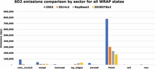
Figures 2 and 3 display the total NO_X and SO₂ U.S. anthropogenic emissions by major source sector across the 13 contiguous WRAP states for the 2002 Hindcast, 2014v2, RepBase2 and 2028OTBa2 emission scenarios. From the 2002 Hindcast scenario, total WRAP states anthropogenic NO_X emissions are estimated to be reduced by −37% and −64% for the, respectively, RepBase2 and 2028OTBa2 emission scenarios. All source sectors are estimated to have reductions in NO_X emissions from 2002 Hindcast levels with the exception of non-point oil and gas whose NO_X emissions are estimated to increase by 64% and 42% for RepBase2 and 2028OTBa2, respectively. Most (77–89%) of the SO₂ emissions in the WRAP states come from the point source sector. RepBase2 and 2028OTBa2 SO₂ emissions are reduced −71% and −76% from the 2002 Hindcast levels driven by the point source SO₂ reductions. The RepBase2 and 2028OTBa2 non-point oil and gas SO₂ emissions are increased by over 2,000%, while Commercial Marine Vessel (CMV) SO₂ emissions are reduced 99% from 2002 Hindcast levels.

Figure 2. Comparison of anthropogenic NO_X emissions for the 2002 Hindcast, 2014v2, RepBase2, and 2028otba2 emission scenario across 13 contiguous WRAP states.

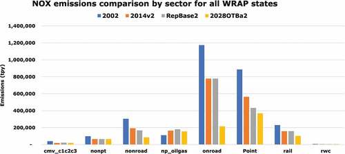
Figure 3. Comparison of anthropogenic SO₂ emissions for the 2002 Hindcast, 2014v2, RepBase2, and 2028otba2 emission scenario across 13 contiguous WRAP states.

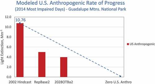
Figure 4 shows the URP Glidepath (solid line) for the Guadalupe Mountains (GUMO1) IMPROVE monitoring site that starts at the 14.6 dv observed 2000–2004 IMPROVE MID baseline and ends at 4.8 dv natural conditions end point in 2064. Also shown are the adjusted Glidepaths (dashed lines) that account for the contributions of international emissions alone and international plus Rx fire emissions in the 2064 endpoint. GUMO1 is close to the Mexican border so this site has a large contribution of about 5 dv from Mexican anthropogenic emissions. Rx fire is very small at GUMO1 so the two dashed lines are almost on top of each other. The projected 2028 visibility using the 3 projections methods ranges from 12.1 to 12.2 dv and lie between the URP Glidepath and adjusted Glidepath. Figure 5 shows the U.S. anthropogenic RoP slope line at GUMO1 using days from the 2014 IMPROVE MID starting with the CAMx PSAT 2002 U.S. anthropogenic emissions contribution at 10.76 Mm⁻¹ and going to 0 Mm⁻¹ in 2064. The 2028OTBa2 U.S. anthropogenic emissions extinction is 3.98 Mm⁻¹ that lies below the RoP slope line at 2028 (4.51 Mm⁻¹) showing that GUMO1 is on a path toward no U.S. manmade impairment in 2064.

Figure 4. URP Glidepath and adjusted Glidepath for the GUMO1 IMPROVE site representing Guadalupe Mountains, Texas and Carlsbad Caverns, New Mexico CIAs and projected 2028 MID visibility using the three projection methods (Source: WRAP TSS Modeling Express Tools Chart 5).

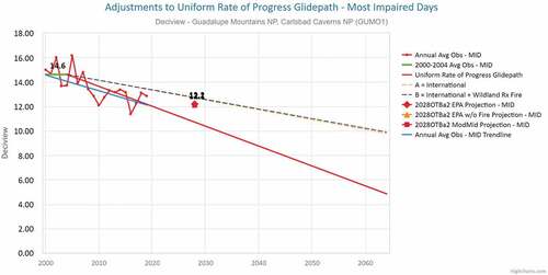
Figure 5. U.S. anthropogenic emissions RoP slope at GUMO2 IMPROVE site with U.S. anthropogenic emissions contributions for RepBase2 (circa 2016) and 2028otba2 below the RoP slope. (Source: Data from WRAP TSS Modeling Express Tools Chart 7).

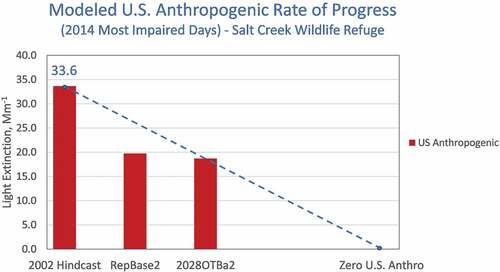
Figures 6 and 7 display another comparison of the URP and adjusted Glidepaths with the U.S. anthropogenic emissions RoP slope line at the Salt Creek, New Mexico CIA. In this case, the projected 2028 visibility for the MID (14.6 dv) lies above both the URP and adjusted Glidepaths. However, the 2028OTBa2 U.S. anthropogenic emissions extinction lies on the RoP slope line at 2028 (19.5 Mm⁻¹).

Figure 6. URP Glidepath and adjusted Glidepath for the Salt Creek, New Mexico (SACR1) IMPROVE site and projected 2028 MID visibility using the three projection methods (Source: WRAP TSS Modeling Express Tools Chart 5).

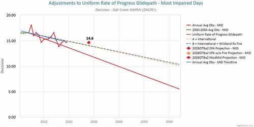
Figure 7. U.S. anthropogenic emissions RoP slope at SACR1 IMPROVE site with U.S. Anthropogenic emissions extinction for RepBase2 (circa 2016) below the RoP slope and 2028otba2 (19.5 Mm ⁻¹) right on the RoP slope. (Source: Data from WRAP TSS Modeling Express Tools Chart 7).

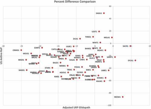
Figure 8 compares the percent difference between the 2028 visibility projection and the 2028 target from the U.S. anthropogenic RoP slope (y-axis) and the URP Glidepath (×-axis) approaches for assessing visibility progress. Of the 117 CIAs in the western U.S. examined, the 2028 visibility projection is below the U.S. anthropogenic RoP slope line for 111 of the CIAs with 6 CIAs being above the RoP slope. The 2028 visibility projection is below the URP Glidepath at 2028 for 63 of the CIAs and above it for 54 CIAs so almost half of the CIAs have 2028 projections that fail to show progress toward natural conditions in 2064 even though the contributions of U.S. manmade emissions are showing progress. Figure 9 is similar to Figure 8 only comparing against the adjusted Glidepath where estimates of visibility due to international and Rx fire emissions have been added to the 2016 natural conditions end-point. The 2028 visibility projections are below the adjusted Glidepath for most CIAs with 4 CIAs being above the adjusted Glidepath. Of the 6 CIAs with 2028 U.S. anthropogenic extinction above the RoP slope line at 2028, three are CIAs in western North Dakota and eastern Montana in the Williston oil and gas basin where oil and gas production was almost nonexistent during the 2000–2004 baseline period. It was only after fracking was in widespread use that opened up the Bakken formation to development so that emissions from oil and gas in the Williston Basin have grown substantially. Gebhart et al. (2018) report near zero VOC and NO_X emissions due to petroleum and related industries in 2002 to almost, respectively, 500,000 and 40,000 tons per year in 2015. So, the 2028 visibility projection being above the U.S. anthropogenic RoP slope line at 2028 makes sense given the higher current and future year local oil and gas emissions than in the 2000–2004 baseline.

Figure 8. Percent difference between 2028 visibility projection and the 2028 target from the URP Glidepath and U.S. anthropogenic emissions RoP slope line using the EPA default projection method.

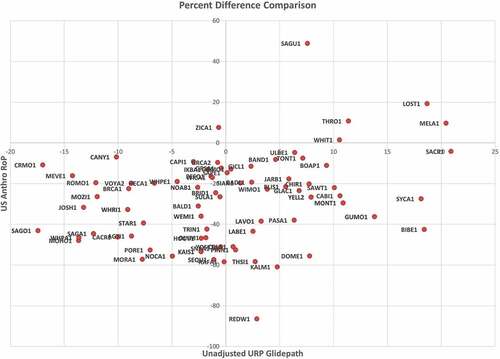
Figure 9. Percent difference between 2028 visibility projection and the 2028 target from the adjusted Glidepath and U.S. anthropogenic emissions RoP slope line using the EPA default projection method.

The procedures used to develop the IMPROVE MID and construct the URP and adjusted Glidepaths for comparison with the 2028 visibility projections to determine whether visibility impairment at the CIA is on a path toward natural conditions in 2064 have numerous uncertainties and inconsistencies:

• The statistical procedure (U.S. EPA, 2018a) used to identify the IMPROVE MID using elevated measured carbon and crustal concentrations to infer the presence of fires and WBD resulting in most (except for routine natural conditions) of the extinction due to AmmSO4 and AmmNO3 defined as anthropogenic in origin is uncertain. Natural fires, lightning, and biogenic soil NO_X emissions also occur that form AmmNO3 extinction that is not anthropogenic in origin. AmmSO4 extinction also has natural sources including oceanic Dimethyl Sulfide (DMS) and geogenic sources. In fact, for Hawaii U.S. EPA has developed a volcanic adjusted (VADJ) MID that screens out high AmmSO4 extinction days due to volcano emission impacts using a similar approach as used for wildfires and dust impacts for the MID (U.S. EPA, 2021b) and Alaska is using a similar approach in their RHR SIP to screen out AmmSO4 visibility impacts from volcano emissions. The U.S. anthropogenic emissions RoP approach for showing visibility progress would be particularly valuable for Class I areas in Hawaii and Alaska where the U.S. anthropogenic emissions component of visibility degradation is dwarfed by international and volcanic emissions.

• The EPA method for identifying the episodic wildfires and WBD events relies on the assumption that carbon and crustal material that are above an historical year lowest 95%ile at a CIA are impacted by, respectively, wildfire and WBD events and that threshold value can be applied for all years at that CIA. This can underestimate the number of natural episodic events at western CIAs that have frequent wildfires or WBD events and overestimate the number of natural episodic events at some eastern CIAs with low or even no impacts from wildfires or WBD. For IMPROVE sites and years with large amounts of wildfire impacts, there are clearly fire impacts on some of the MID as evident with elevated carbon concentrations during the fire season. There are also CIAs that appear to have dust impacts on the IMPROVE MID (e.g., Canyonlands in 2014).

• The 2064 Natural Conditions MID endpoint for the URP Glidepath is based on analysis of 2000–2014 IMPROVE data (Copeland, Pitchford and Ames, 2008) and is also uncertain. The routine natural haze estimate is based on Trijonis et al. (1990) that evaluates available monitoring data in the 1970s and 1980s and reports a single annual average natural haze estimate for all sites in the western U.S. The EPA statistical method assumes that daily variability in natural haze varies proportionally to daily total haze, but this assumption is not tested and may not accurately account for daily and seasonal variability in natural haze.

• The adjustments to the URP Glidepath 2064 endpoint to account for contributions of international emissions and Rx fire are also questionable as emission estimates for both source categories are highly uncertain and their impacts 40 years in the future are impossible to predict.

• The modeling results can have fire impacts on the IMPROVE MID that are inconsistent with the assumptions used in calculating the IMPROVE MID and make the model RRFs less responsive to U.S emissions reductions because fires are typically assumed to be constant between the current and future year resulting in RRFs for OMC being approximately unity. This will cause the model to understate the future year MID visibility benefits due to anthropogenic emission reductions.

Many U.S. anthropogenic emissions (e.g., power plants with continuous emissions monitoring systems) are better known than wildfire, prescribed burn, natural and international emissions, and likely less uncertain than the estimated natural conditions that are used in the current MID URP Glidepath Regional Haze analysis. U.S. anthropogenic emissions are also essentially the only component that can be controlled to reduce visibility impairment at CIAs and the exact source of visibility impairment that Congress intended to be mitigated in the 1977 CAAA. The U.S. anthropogenic emissions RoP analysis directly estimates the rate that manmade visibility impairment due to U.S. anthropogenic emissions is being reduced from the 2000–2004 (2002) Baseline to an ultimate goal of no U.S. anthropogenic emissions impairment in 2064. The URP and adjusted Glidepath approach are attempting to back into the U.S. anthropogenic emissions contribution to visibility by starting with total visibility from the measured IMPROVE data and backing out contributions estimated to be due to routine natural sources and episodic fire and WBD natural impacts. Additional adjustments for international anthropogenic and Rx fire emissions are extremely uncertain and much less reliable than the U.S. anthropogenic emissions that the RoP approach uses directly. The U.S. anthropogenic emissions RoP analysis also has uncertainties and limitations as it is based on absolute modeling results that have uncertain meteorological, emissions and transport inputs as well as uncertainties associated with the backcast 2002 Hindcast emissions scenario and the burden of having to conduct computationally extensive source apportionment modeling.

Results of the dynamic evaluation

The CAMx simulation of the 2002 Hindcast emissions scenario also allowed WRAP to conduct a Dynamic Evaluation of the future year visibility projection techniques used with the WRAP 2014 modeling platform. EPA’s photochemical modeling guidance lists four types of model performance evaluation (U.S. EPA, 2018c):

• Operational Evaluation that evaluates the model’s ability to reproduce concurrent observations for the base modeling year;

• Diagnostic Evaluation is a process-oriented evaluation that evaluates the model’s ability to reproduce observed meteorological, chemical, and physical processes that lead to the air quality issues being examined;

• Dynamic Evaluation evaluates the model’s ability to simulate the observed changes in concentrations/visibility in response to changes in emissions; and

• Probabilistic Evaluation attempts to assess the level of confidence in the model predictions through techniques such as ensemble model simulations.

The Operational and Diagnostic Evaluation of the WRAP 2014 modeling platform are documented in webpages on the WRAP TSS website cited earlier. A Probabilistic Evaluation is very resource intensive, rarely performed and was not conducted for the WRAP 2014 platform. True Dynamic Evaluations are also resource intensive and difficult to interpret due to year-to-year variations in meteorology and resultant concentrations that can interfere with the signal of the change in concentrations in response to changes in emissions (Dennis et al., 2010) as well as difficulties in constructing modeling emissions inventories for historical years (Thunis and Clappier, 2014). Several Dynamic Evaluations have been performed and documented in the open literature. For example, Turnock et al., (2015) compared modeled and observed changes in aerosols and surface radiation over Europe between 1960 and 2009. Pozzer et al. (2015) compared aerosol optical depth (AOD) from observations and model simulations between 2001 and 2010. Boys et al., (2014) compared 15 years of GEOS-Chem modeled and satellite observed PM_2.5 concentrations over 15 years. Chin et al., (2014) compared multi-decadal (1980–2009) changes in observed and modeled aerosol concentrations. The NO_X SIP call resulted in a reduction in point source NO_X emissions in the eastern U.S. between 2002 and 2004/2005/2006 that was used in Dynamic Evaluations by Gilliland et al, (2008), Napelenok et al. (2011), Zhou et al., (2013) and Foley et al, (2015a, 2015b) to determine whether photochemical model’s ozone concentrations responded to the sudden drop in regional NO_X emissions the same way as observed. Karamchandani et al., (2017) evaluated the ability of photochemical models to reproduce the observed changes in ozone from 1990 to 2014/2015 using two recent databases used to define ozone control plans in Southern California.

WRAP performed a limited retrospective Dynamic Evaluation of their 2014 modeling platform and methods used for projecting the observed 2014–2018 IMPROVE MID visibility to 2028 using the RepBase2 and 2028OTBa2 CAMx modeling results (RRF = 2028OTBa2/RepBase2). The Dynamic Evaluation did a “backward projection” using the observed 2014–2018 IMPROVE MID that was projected to 2002 using the RepBase2 and 2002 Hindcast CAMx modeling results (RRF = 2002 Hindcast/RepBase2) and the EPA, EPAwoF, and ModMID visibility projection approaches. In addition, a Dynamic Evaluation “forward projection” was also performed that projected the observed 2000–2004 IMPROVE MID to circa 2016 using the 2002 Hindcast and RepBase2 CAMx modeling results (RRF = RepBase2/2002 Hindcast).

The Dynamic Evaluation used graphical displays (e.g., scatter plots) and statistical performance metrics to evaluate how well the WRAP modeling platform and three projection methods could reproduce the observed changes in visibility on the MID over time (i.e., between 2000–2004 and 2014–2018). The statistical performance metrics were the normalized mean bias (NMB) and error (NME) and correlation coefficient (r) that are defined as follows:

$\mathrm{N}\mathrm{o}\mathrm{r}\mathrm{m}\mathrm{a}\mathrm{l}\mathrm{i}\mathrm{z}\mathrm{e}\mathrm{d}\mathrm{M}\mathrm{e}\mathrm{a}\mathrm{n}\mathrm{B}\mathrm{i}\mathrm{a}\mathrm{s}\left(\mathrm{N}\mathrm{M}\mathrm{B}\right)=\frac{\sum _1^n(M-o)}{\sum _1^n(o)}$

$\mathrm{N}\mathrm{o}\mathrm{r}\mathrm{m}\mathrm{a}\mathrm{l}\mathrm{i}\mathrm{z}\mathrm{e}\mathrm{d}\mathrm{E}\mathrm{r}\mathrm{r}\mathrm{o}\mathrm{r}\left(\mathrm{N}\mathrm{M}\mathrm{E}\right)=\frac{\sum _1^n\left|M-o\right|}{\sum _1^n(o)}$

$\mathrm{C}\mathrm{o}\mathrm{r}\mathrm{r}\mathrm{e}\mathrm{l}\mathrm{a}\mathrm{t}\mathrm{i}\mathrm{o}\mathrm{n}\left(\mathrm{r}\right)=\frac{1}{(n-1)}\sum _1^n\left(\left(\frac{o-\bar{o}}{{\sigma }_o}\right)\ast \left(\frac{M-\bar{M}}{{\sigma }_m}\right)\right)$

where O are the observed and M are the modeled projected visibility for the MID.

Emery et al. (2016) has developed performance goals and criteria for photochemical models and the NMB, NME, and r statistical performance metrics based on an analysis of papers in the peer-reviewed Journals from 2005 to 2015. Performance goals indicate statistical values that about a third of the top performing past applications have met and should be viewed as the best a model can be expected to achieve. Performance criteria indicate statistical values that about two-thirds of past models have achieved and should be viewed as what a majority of past applications have achieved. Although performance goals and criteria are not presented for visibility, the ones for PM_2.5 are appropriate for comparing against visibility as they represent the same species just a different weighting (by extinction instead of mass). The performance goals and criteria for PM_2.5 and SO₄ are the same and are provided for NMB (<±10% and <±30%), NME (<35% and <50%), and r (>0.70 and >0.40). The goals and criteria for other PM species are relaxed from those for PM_2.5 and SO₄for example, NMB goals and criteria for NO₃ (<±15% and <±65%), OMC (<±15% and <±50%) and EC (<±20% and <±40%).

The Dynamic Evaluation was conducted for total visibility, expressed as both deciview (DV) and total extinction (TBext), as well as extinction for each of the six PM species that are used to estimate visibility from the IMPROVE measurements and CAMx modeling results. Table 1 shows the NMB, NME, and r performance statistics for the backward and forward projection Dynamic Evaluation and DV, TBext and extinction due to AmmSO4, AmmNO3, OMC, and EC. Figures 10 and 11 display scatter plots of TBext for the, respectively, backward and forward projection evaluations. For DV, the ModMID projection approach has the lowest NMB for both the forward and backward projection approaches (+0.2% and +2.1%) with EPAwoF approach next best (−1.8% and 3.4%) and EPA projection approach having the highest NMB (−3.2% and +4.7%). Similar rankings among the three projection methods DV Dynamic Evaluation are seen for NME as well as NMB and NME for TBext, which is not surprising since TBext is directly related to DV [DV = 10 ln (TBext/10)]. The correlation coefficients are very high (>0.9) for DV and TBext and the three projection methods, which is not surprising since the same CIAs tend to have relatively higher and lower visibility extinction for both the 2000–2004 and 2014–2018 time periods. This is shown in the Dynamic Evaluation scatter plots in Figures 10 and 11 where TBext for the MID range from 20 to 120 Mm⁻¹ in 2000–2004 and from 15 to 70 Mm⁻¹ in 2014–2018. When doing the backward projection, the DV and TBext have an underestimation bias (i.e., the projected 2002 MID tends to be lower than was observed during 2000–2004). Whereas, when doing the forward projection there is a positive bias in DV and TBext. The 2014 platform and projections techniques tend to have lower magnitude bias and less scatter for the backward projection than the forward projection, which may be partly due to the 2014 meteorology used is connected to the observed 2014–2018 IMPROVE MID used as the starting point for the backward projection while the 2014 meteorology is not connected to the observed 2000–2004 IMPROVE MID used as the starting point for the forward projection Dynamic Evaluation. Overall, the Dynamic Evaluation for DV and TBext is quite good with low NMB (≤±6.1%) and NME (≤9.0%) and high correlation that meet the PM_2.5 performance goals.

Figure 10. Dynamic Evaluation for total extinction (TBext) of the WRAP 2014 modeling platform and three visibility projection approaches for the backward evaluation that projected the observed 2014–2018 IMPROVE to 2002 and compared the projected 2002 MID visibility to the observed 2000–2004 IMPROVE MID.

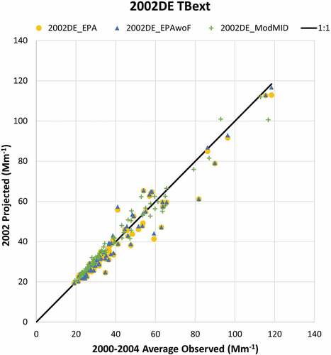
Figure 11. Dynamic Evaluation for total extinction (TBext) of the WRAP 2014 modeling platform and three visibility projection approaches for the forward evaluation that projected the observed 2000–2004 IMPROVE to RepBase2 (circa 2016) and compared the projected RepBase2 MID visibility to the observed 2014–2018 IMPROVE MID.

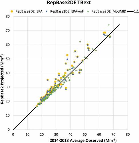
Table 1. Dynamic Evaluation performance statistics on the ability of the WRAP 2014 modeling platform and three projection approaches to match the observed IMPROVE MID for decivew (DV), total extinction (TBext), ammonium sulfate (AmmSO4), ammonium nitrate (AmmNO3), organic matter carbon (OMC), and elemental carbon (EC) for backward and forward projection approaches using the RepBase2 and 2002 Hindcast CAMx modeling results.

Species/ Metric	Backward Projection Projected 2002DE Observed 2000-2004			Forward Projection Projected RepBase2DE Observed 2014-2018
DV	EPA	EPAwoF	ModMID	EPA	EPAwoF	ModMID
NMB	−3.2%	−1.8%	0.2%	4.7%	3.4%	2.1%
NME	6.2%	6.0%	5.6%	7.0%	6.6%	6.3%
R	0.97	0.97	0.97	0.97	0.96	0.96
TBext	EPA	EPAwoF	ModMID	EPA	EPAwoF	ModMID
NMB	−4.6%	−2.7%	−1.2%	6.1%	4.7%	3.9%
NME	8.7%	8.4%	8.7%	9.0%	8.3%	8.5%
r	0.97	0.97	0.97	0.96	0.96	0.94
AmmSO4	EPA	EPAwoF	ModMID	EPA	EPAwoF	ModMID
NMB	7.8%	11.6%	16.1%	−4.5%	−7.2%	−12.9%
NME	16.6%	18.5%	21.1%	14.5%	15.1%	17.0%
r	0.96	0.96	0.95	0.95	0.95	0.95
AmmNO3	EPA	EPAwoF	ModMID	EPA	EPAwoF	ModMID
NMB	−26.1%	−25.5%	−26.7%	39.8%	38.6%	42.2%
NME	28.5%	28.1%	29.1%	42.1%	41.1%	44.9%
r	0.96	0.96	0.95	0.94	0.94	0.92
OMC	EPA	EPAwoF	ModMID	EPA	EPAwoF	ModMID
NMB	−9.1%	−5.9%	−3.6%	10.2%	6.9%	6.7%
NME	14.2%	14.9%	18.1%	15.6%	15.8%	19.9%
r	0.93	0.92	0.89	0.92	0.918	0.81
EC	EPA	EPAwoF	ModMID	EPA	EPAwoF	ModMID
NMB	−22.4%	−16.9%	−16.1%	32.8%	25.9%	33.0%
NME	26.2%	25.0%	26.3%	37.2%	34.6%	43.5%
r	0.75	0.728	0.67	0.74	0.68	0.43

The Dynamic Evaluation for AmmSO4 extinction is also fairly good (Table 1) with NMB and NME that are low, but not as low as DV/TBext that have the advantage of adding Rayleigh background to both the observed and predicted values that reduces bias and error. The EPA and EPAwoF projections approaches (NMB from −4.5% to +11.2%) are clearly performing better than the ModMID approach (NMB of +16.1% and −12.9%) for projecting AmmSO4 extinction with the EPA approach performing a little better than EPAwoF and meeting the performance goals for both the forward and backward projection. The Dynamic Evaluation performance for AmmNO3 extinction is not nearly as good as seen for DV, TBext, and AmmSO4 with NMB for the backward and forward projections of approximately −26% and +40%, respectively, that fail to achieve the ±15% NO3 performance goal but do achieve the NO3 performance criteria (Emery et al. 2016). Many CIAs have very low (<4 Mm⁻¹) extinction due to AmmNO3 so small discrepancies can lead to big relative bias performance statistics. All three projection approaches have poorer Dynamic Evaluation performance statistics for AmmNO3 extinction.

For projecting OMC extinction, the ModMID method has the lowest (−3.6% and +6.7%) NMB followed by the EPAwoF (−5.9% and +6.9%) and then EPA (−9.1% and +10.2%) with all three projection methods achieving the OMC performance goals for NMB, NME, and r (Table 1). As the OMC is the species most affected by fires and the fires during 2014–2018 and 2000–2004 are likely very different, it is not surprising that the two projection methods that eliminate the contributions of fires in the RRFs (EPAwoF and ModMID) perform better for OMC than the method that did not (EPA). Although the ModMID approach has the lowest NMB for OMC extinction, it has the highest NME. The EC extinction has higher NMB and NME than OMC, which is due in part to having many low (<3 Mm⁻¹) EC extinction values. The EPAwoF approach appears to perform best for projecting EC extinction.

the EPAwoF projection approach appears to be consistently performing at or near the best of the three projection methods and is consistent with EPA guidance (U.S. EPA, 2018c) and the goals of the IMPROVE MID to limit influences of wildfires (U.S. EPA, 2018a) on the days in the MID.

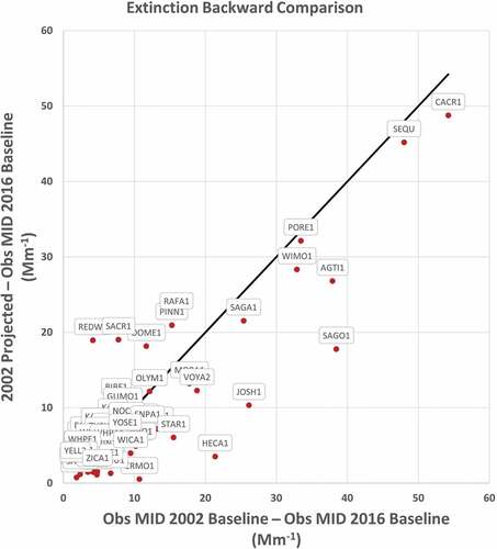
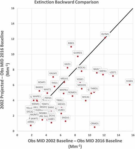
Figure 12 displays a scatter plot the difference in total extinction between the observed IMPROVE 2014–2018 MID and the observed IMPROVE 2000–2004 MID versus the observed IMPROVE 2014–2018 MID and the predicted 2002 visibility MID using the EPA default projection approach. Each point in the scatter plot is labeled by the IMPROVE site’s short name whose locations can be found on the IMPROVE website (http://vista.cira.colostate.edu/Improve/improve-program/). The backward model projected change in extinction matches the observed change reasonably well with an underestimation tendency that is approximately −20% on average. Most (74%) sites have modeled changes in extinction that are within a factor of two of the observed change and approximately half the sites are within a factor of 1.5. The underestimation of the change in extinction is partly due to keeping international emissions constant at current 2014 levels in the CAMx 2002 hindcast simulation when they were likely lower in 2002 than in 2014. The largest increase in extinction between 2014–2018 and 2000–2004 occurs at the Caney Creek (CACR1) Arkansas site that is influenced by the higher AmmSO4 levels in the eastern U.S. than sites in the western U.S. and at Sequoia (SEQU1) California site that is affected by emissions from California’s San Joaquin Valley with both the observed and backward projection estimating an approximately 50 Mm⁻¹ increase in extinction at these two sites. The four IMPROVE sites in southern California (AGT1, JOSH1, SAGA1, and SAGO1) have a larger observed increase in extinction from 2014–2018 to 2000–2004 (25–40 Mm⁻¹) than modeled (10–30 Mm⁻¹) because the backward projection understates the level of AmmNO3 extinction in 2000–2004 (e.g., −26% bias in Table 1) and these southern California sites have a higher fraction of extinction due to AmmNO3 in the MID than most other sites. Hells Canyon (HECA1) Idaho is another site with a higher fraction of AmmNO3 extinction and its observed increase in extinction (21.4 Mm⁻¹) is also much higher than the backward projection (3.5 Mm⁻¹). On the other hand, the backward projection at the Redwood (REDW1) site on the coast of northern California has a much higher modeled increase in extinction from 2014–2018 to 2000–2004 (18.9 Mm⁻¹) than observed (4.2 Mm⁻¹), which may be due to model performance issues as AmmSO4 was overestimated at REDW1. The backward projected also overstates the amount of extinction increase versus observed at the San Rafael Wilderness (RAFA1) site on the coast north of southern California (22.3 vs. 16.0 Mm⁻¹) and the Kalmiopsis (KALM1) site on the coast in southern Oregon (7.1 vs. 5.0 Mm⁻¹) but the overestimation is not as large as at REDW1. But the backward projection matches the observed changes in extinction very well at the Point Reyes (PORE1) coastal site north of San Francisco (33.5 vs. 32.1 Mm⁻¹) as well as the Olympic (OLYM1) site near the coast west of Seattle (12.2 vs. 12.2 Mm⁻¹).

Figure 12. Comparison of changes in extinction between the observed IMPROVE 2014–2018 MID extinction and the observed IMPROVE 2000–2004 MID extinction (×-axis) versus predicted 2002 modeled extinction (y-axis) using the CAMx RepBase2 and 2002 hindcast backwards projection.

Figure 13 is the same data as plotted in Figure 12 only the maximum for the scale on the two axis has been reduced from 60 to 16 Mm⁻¹ so that the data for sites with smaller increases in extinction between 2014–2018 and 2000–2004 can be examined. The backward projected increase in extinction is usually within a factor of two of the observed but there are some sites in geographic areas where the underestimation exceeds a factor of two. The observed increase in extinction at Craters of the Moon (CRMO1), Idaho (10.7 Mm⁻¹) is 20 times higher than the backward projection (0.5 Mm⁻¹) with the observed increase in extinction underestimated by the backward projection at several other nearby sites, such as STAR1 and MOHO1 in Oregon and HECA1 site discussed above.

Figure 13. Comparison of changes in extinction between the observed IMPROVE 2014–2018 MID extinction and the observed IMPROVE 2000–2004 MID extinction (×-axis) versus predicted 2002 modeled extinction (y-axis) using the CAMx RepBase2 and 2002 hindcast backwards projection using a smaller scale than in Figure 12.

There are numerous uncertainties in the WRAP Dynamic Evaluation, including:

• International emissions are kept constant at 2014 levels in the 2002 Hindcast and RepBase2 CAMx simulations.

• Meteorological conditions are kept constant using 2014 WRF simulation.

• Large sulfate overestimation at western coastal sites due to boundary conditions and/or overstated DMS emissions and/or overstated commercial marine emissions.

• At times large underestimation of coarse matter in the southwest U.S. due to poor characterization of windblown dust emissions.

• Additional model performance issues that varied over space and time.

Future studies should perform more comprehensive Dynamic Evaluations using year-specific international and natural emissions and meteorological conditions. It should be noted that the previous Dynamic Evaluations for PM and ozone cited above focused on areas with high concentrations of PM or ozone. A Dynamic Evaluation is more challenging for most Class I areas in the western U.S. that have very low concentrations of PM even on the MID.

Discussion and conclusions

EPA guidance recommends use of a statistical analysis to identify the IMROVE MID to track progress from the 2000–2004 baseline to recent years (e.g., 2014–2018), then processes the IMPROVE data using their method for use by the states, and to then use model simulations to estimate additional progress from 2014–2018 to the 2028 milestone year. Specifically, the EPA method evaluates progress in reducing U.S. contributions to impairment indirectly by subtracting estimates of natural haze from the total measured extinction and by adjusting the URP Glidepath for estimates of international impairment. However, international emissions are assumed to be constant in the EPA method even though there have been substantial increases in some (e.g., Asia) international emissions since the 2002 baseline year. Because estimates of natural haze and international impairment have large uncertainties, this indirect method of estimating U.S. contributions to impairment transfers the uncertainties in estimates of natural haze and international impairment to the estimate of U.S. anthropogenic impairment. Because of this uncertainty, the EPA statistical analysis of progress in reducing impairment from 2002 to 2016 may not accurately measure reductions in U.S. contributions to impairment. An alternate approach is to use photochemical grid models to estimate U.S. impairment in 2002 and 2028 and to calculate a U.S. anthropogenic Rate of Progress (RoP). Because trends in many of U.S. anthropogenic emission source sectors are better known, the direct estimate of the RoP may have less uncertainty than the indirect approach which relies on uncertain estimates of natural haze and international impairment. However, the US anthropogenic approach is not without uncertainties as backcasting emissions is uncertain and models have their own uncertainties. The ROP approach also has the additional burden of conducting photochemical grid model source apportionment simulations. However, the RoP approach may be more accurate and reliable for evaluating progress toward no U.S. anthropogenic emissions impairment, especially for future regional haze SIPs that states are required to submit for the 2038, 2048, and 2058 benchmark years when the U.S. anthropogenic emissions are expected to be reduced and swamped by natural sources of haze.

We have shown that the U.S. anthropogenic emissions RoP is a useful alternative approach for evaluating whether visibility at a CIA is on a path toward no U.S. manmade impairment in 2064 that compliments the URP Glidepath and adjusted Glidepath approaches. It does not take the place of the IMPROVE MID or similar metric based on observations that is needed to track visibility progress of the IMPROVE observations over time. But the RoP may provide a more certain and direct approach for evaluating the progress of U.S. manmade visibility impairment without relying on uncertainties associated with the IMPROVE MID approach, which use measured carbon and crustal material to infer contributions from wildfire and dust emissions, uncertainties in international anthropogenic emissions and wildland prescribed burns, and the uncertain and unknowable natural conditions used as a 2064 end-point. The U.S. anthropogenic emissions RoP analysis also has uncertainties foremost among them is the backcast 2002 Hindcast emissions and the inherent uncertainties associated with a photochemical grid model (e.g., emissions, meteorology, pollutant transport, and model formulation) and uncertainties in the particulate matter source apportionment tool. The use of the URP and adjusted Glidepaths to evaluate the model projected RPG also has the inherent uncertainties associated with a photochemical grid model.

The 2002 Hindcast simulation also afforded the opportunity to conduct a Dynamic Evaluation to evaluate how well the WRAP 2014 modeling platform and associated visibility projection methods could replicate the observed changes in visibility over time. The projection methods demonstrated some skill in projecting deciview and total extinction as well as extinction due to ammonium sulfate and organic mass carbon and less skill in projecting extinction due to ammonium nitrate and elemental carbon that can have very low concentrations at times at some CIAs. Of the three projection methods evaluated, the EPAwoF projection approach performed the best when analyzing across all the Dynamic Evaluation performance metrics.

Acknowledgment

The results of this paper were made possible by the air quality and emissions modeling team at Ramboll of Tejas Shah, Chao-Jung Chien, Yesica Alvarez and Pradeepa Vennam under the direction of the co-authors and the WRAP Regional Technical Operations Work Group with co-chairs Mike Barna of the National Park Service and Kevin Briggs of the Colorado Department of Public Health and Environment. The authors would also like to acknowledge Shawn McClure of Colorado State University who implemented the visualization of the modeling results on the WRAP Technical Support System. This paper does not reflect EPA policy, guidance or recommendations.

Disclosure statement

No potential conflict of interest was reported by the authors.

Data availability statement

The data that support the findings of this study are available on the Intermountain West Data Warehouse (IWDW) and Western Regional Air Partnership (WRAP) Technical Support System (TSS) websites. Specifically, the CAMx 2014 modeling platform files for the 2014v2, RepBase2, 2029OTBa2 and 2002 Hindcast emissions scenarios can be downloaded from the IWDW website (https://views.cira.colostate.edu/iwdw/RequestData/Default.aspx) with the definitions of the scenarios also available on the IWDW website (https://views.cira.colostate.edu/iwdw/Modeling/Platforms.aspx). The graphics and data used in the URP Glidepath displays are available from Chart 4 and the data used in the U.S. Anthropogenic Emissions Rate of Progress (RoP) displays are available in Chart 6 of the WRAP TSS Modeling Express Tools website (https://views.cira.colostate.edu/tssv2/Express/ModelingTools.aspx).

References

- Air Sciences. 2020. Fire emission inventories for regional haze planning: Methods and results. Air Sciences, Inc, Portland, Oregon. April. http://wrapair2.org/pdf/fswg_rhp_fire-ei_final_report_20200519_FINAL.PDF
- Bar-Ilan, A., R. Friesen, A. Pollack, and A. Hoats. 2007. WRAP area source emissions inventory projections and control strategy evaluation, phase II. ENVIRON International Corporation, Novato, California. September. https://www.wrapair.org/forums/ogwg/documents/2007-10_Phase_II_O&G_Final)Report(v10-07%20rev.s).pdf
- Bey, I., D. Jacob, R. Yantosca, J. Logan, B. Field, A. Fiore, Q. Li, H. Liu, L. Mickley, and M. Schultz. 2001. Global modeling of tropospheric chemistry with assimilated meteorology: Model description and evaluation. J. Geophys. Res. Atmos. 106 (D19): 23073–95, October 16. doi:10.1029/2001JD000807.
- Bowden, J., K. Talgo, and Z. Adelman. 2016. Western-State Air Quality Modeling Study (WAQS) – weather research forecast 2014 meteorological model Application/Evaluation. University of North Carolina at Chapel Hill – Institute for the Environment. January 1. http://views.cira.colostate.edu/wiki/Attachments/Modeling/WAQS_2014_WRF_MPE_January2016.pdf
- Boys, B., R. Martin, A. van Donkelaar, R. MacDonell, N. Hsu, M. Cooper, R. Yantosca, Z. Lu, D. Streets, Q. Zhang, et al. 2014. Fifteen-year global time series of satellite-derived fine particulate matter. Environ. Sci. Technol. 48 (19):11109–18. doi:10.1021/es502113p.
- CAAA. 1977. Section 7491 of the 1997 Clean Air Act Amendments. United States Code, Title 42 – the Public Health and Welfare, Chapter 85 – Air Pollution Prevention and Control, Subchapter I – Program and Activities, Part C – Prevention of Significant Deterioration, subpart ii – visibility protection, Sec 7491 – Visibility protection for Federal class areas. https://www.govinfo.gov/content/pkg/USCODE-2013-title42/html/USCODE-2013-title42-chap85-subchapI-partC-subpartii-sec7491.htm
- Chin, M., T. Diehl, Q. Tan, J. Prospero, R. Kahn, L. Remer, H. Yu, A. Sayer, H. Bian, I. Geogdzhayev, et al. 2014. Multi-decadal aerosol variations from 1980 to 2009: A perspective from observations and a global model. Atmos. Chem. Phys. 14 (7):3657–90. doi:10.5194/acp-14-3657-2014.
- Copeland, S., M. Pitchford, and R. Ames. 2008. Regional haze rule natural level estimates using the revised IMPROVE aerosol reconstructed light extinction algorithm. Presented at: Air & Waste Management Association Aerosol & Atmospheric Optics Visual Air Quality and Radiation specialty conference in Moab, Utah, April. Final Paper #48. http://vista.cira.colostate.edu/improve/publications/graylit/032_NaturalCondIIpaper/Copeland_etal_NaturalConditionsII_Description.pdf
- Dennis, R., T. Fox, M. Fuentes, A. Gilliland, S. Hanna, C. Hogrefe, J. Irwin, S. T. Rao, R. Scheffe, K. Schere, et al. 2010. A framework for evaluating regional-scale numerical photochemical modeling systems. Environ. Fluid Mech. 10 (4):471–89. doi:10.1007/s10652-009-9163-2.
- Emery, C. E., Z. Liu, A. G. Russell, M. T. Odman, G. Yarwood, and N. Kumar. 2016. Recommendations on statistics and benchmarks to assess photochemical model performance. J. Air Waste Manage. Assoc. 67 (5). doi:10.1080/10962247.2016.1265027.
- Foley, K., P. Dolwick, C. Hogrefe, H. Simon, B. Timin, and N. Possiel. 2015b. Dynamic evaluation of CMAQ part II: Evaluation of relative response factor metrics for ozone attainment demonstrations. Atmos. Environ. 103:188–95. doi:10.1016/j.atmosenv.2014.12.039.
- Foley, K., C. Hogrefe, G. Pouliot, N. Possiel, S. Roselle, H. Simon, and B. Timin. 2015a. Dynamic evaluation of CMAQ part I: Separating the effects of changing emissions and changing meteorology on ozone levels between 2002 and 2005 in the eastern US. Atmos. Environ. 103:247–55. doi:10.1016/j.atmosenv.2014.12.038.
- Gebhart, K. A., D. E. Day, A. J. Prenni, B. A. Schichtel, J. L. Hand, and A. R. Evanoski-Cole. 2018. Visibility impacts at Class I areas near the Bakken oil and gas development. J. Air Waste Manag. Assoc. 68 (5):477–93. doi:10.1080/10962247.2018.1429334.
- Gilliland, A., C. Hogrefe, R. Pinder, J. Godowitch, K. Foley, and S. T. Rao. 2008. Dynamic evaluation of regional air quality models: Assessing changes in O3 stemming from changes in emissions and meteorology. Atmos. Environ. 42 (20):5110–23. doi:10.1016/j.atmosenv.2008.02.018.
- Karamchandani, P., R. Morris, A. Wentland, T. Shah, S. Reid, and J. Lester. 2017. Dynamic evaluation of photochemical grid model response to emission changes in the South Coast Air Basin in California. Atmosphere 8 (12):145. doi:10.3390/atmos8080145.
- Keller, C., M. Long, R. Yantosca, A. Da Silva, Pawson, D. Jacob, S. Pawson, and S. Pawson. 2014. HEMCO v1.0: A versatile, ESMF-compliant component for calculating emissions in atmospheric models. Geosci. Model Dev. 7 (4):1409–17. doi:10.5194/gmd-7-1409-2014.
- Koo, B., G. Wilson, R. Morris, A. Dunker, and G. Yarwood. 2009. Comparison of source apportionment and sensitivity analysis in a particulate matter air quality model. Environ. Sci. Technol. 43 (17):6669–75. doi:10.1021/es9008129.
- Napelenok, S., K. Foley, D. Kang, R. Mathur, T. Pierce, and S. T. Rao. 2011. Dynamic evaluation of regional air quality model’s response to emission reductions in the presence of uncertain emission inventories. Atmos. Environ. 45 (24):4091–98. doi:10.1016/j.atmosenv.2011.03.030.
- Nopmongcol, U., Y. Alvarez, J. Jung, J. Grant, N. Kumar, and G. Yarwood. 2017. Source contributions to United States ozone and particulate matter over five decades from 1970 to 2020. Atmos. Environ. 167:116–28. October. doi: 10.1016/j.atmosenv.2017.08.009.
- NRC. 1993. Protecting visibility in National Parks and Wilderness Areas. Washington D.C: The National Academies Press. National Research Council https://www.nap.edu/catalog/2097/protecting-visibility-in-national-parks-and-wilderness-areas.
- Pitchford, M., W. Malm, B. Schichtel, N. Kumar, D. Lowenthal, and J. Hand. 2007. Revised algorithm for estimating light extinction from IMPROVE particle speciation data. J. Air Waste Manage. Assoc. 57 (11):1326–36. doi:10.3155/1047-3289.57.11.1326.
- Pozzer, A., A. de Meij, J. Yoon, H. Tost, A. Georgoulias, and M. Astitha. 2015. AOD trends during 2001–2010 from observations and model simulations. Atmos. Chem. Phys. 15 (10):5521–35. doi:10.5194/acp-15-5521-2015.
- Ramboll. 2020. User’s guide comprehensive air quality model with extensions, version 7.1. Ramboll Environmental and Health. ramboll.com. camx.com. December. https://camx-wp.azurewebsites.net/Files/CAMxUsersGuide_v7.10.pdf
- Skamarock, W. C., J. B. Klemp, J. Dudhia, D. O. Gill, D. M. Barker, M. G. Duda, X.-Y. Huang, W. Wang, and J. G. Powers, 2008. A description of the Advanced Research WRF Version 3. NCAR Technical Note 475. http://www2.mmm.ucar.edu/wrf/users/docs/arw_v3.pdf
- Solomon, P., D. Crumpler, J. Flanagan, R. Jayanty, E. Rickman, and C. McDade. 2014. U.S. National PM 2.5 Chemical Speciation Monitoring Networks—CSN and IMPROVE: Description of networks. J. Air Waste Manage. Assoc. 64 (12):1410–38. doi:10.1080/10962247.2014.956904.
- Thunis, P., and A. Clappier. 2014. Indicators to support the dynamic evaluation of air quality models. Atmos. Environ. 98:402–09. doi:10.1016/j.atmosenv.2014.09.016.
- Turnock, S., D. Spracklen, K. Carslaw, G. Mann, M. Woodhouse, P. Forster, J. Haywood, C. Johnson, M. Dalvi, N. Bellouin, et al. 2015. Modelled and observed changes in aerosols and surface solar radiation over Europe between 1960 and 2009. Atmos. Chem. Phys. 15 (16):9477–500. doi:10.5194/acp-15-9477-2015.
- U.S. EPA. 1999. Regional Haze Regulations, Final Rule. U.S. Environmental Protection Agency. 40 CFR Part 51. Federal Register/Vol. 64, No. 126/Thursday, July 1, 1999, pp. 35714–74. https://www.govinfo.gov/content/pkg/FR-1999-07-01/pdf/99-13941.pdf
- U.S. EPA. 2001. Procedures Document for National Emission Inventory Criteria Air Pollutants 1985-1999. U.S. Environmental Protection Agency, Office of Air Quality Planning and Standards, Research Triangle Park, North Carolina. EPA-454/R-01-006. March. https://www.epa.gov/sites/default/files/2015-07/documents/aerr_final_rule.pdf
- U.S. EPA. 2017. Protection of Visibility Amendments to Requirements for State Plans, Final Rule. U.S. Environmental Protection Agency. 40 CFR Parts 51 and 52. Federal Register/Vol. 82, No. 6/Tuesday, January 10, 2017, pp. 3078–129. https://www.govinfo.gov/content/pkg/FR-2017-01-10/pdf/2017-00268.pdf
- U.S. EPA. 2018a. Technical guidance on tracking visibility progress for the second implementation period of the regional haze Program. U.S. Environmental Protection Agency, Office of Air Quality Planning and Standards, Air Quality Assessment Division, Research Triangle Park, North Carolina. EPA-454/R-18-010. December https://www.epa.gov/sites/default/files/2018-12/documents/technical_guidance_tracking_visibility_progress.pdf
- U.S. EPA. 2018b. 2014 National Emissions Inventory, version 2 Technical Support Document. U.S. Environmental Protection Agency, Office of Air Quality Planning and Standards, Air Quality Assessment Division, Emissions Inventory and Analysis Group. North Carolina: Research Triangle Park. July. https://www.epa.gov/sites/default/files/2018-07/documents/nei2014v2_tsd_05jul2018.pdf
- U.S. EPA. 2018c. Modeling guidance for demonstrating air quality goals for ozone, PM2.5, and regional haze. U.S. Environmental Protection Agency, Office of Air Quality Planning and Standards, Air Assessment Division. Research Triangle Park, NC. EPA 454/R-18-009. November 29. https://www.epa.gov/sites/default/files/2020-10/documents/o3-pm-rh-modeling_guidance-2018.pdf
- U.S. EPA. 2019a. Software for the Modeled Attainment Test – Community Edition. (SMAT0-CE). https://www.epa.gov/scram/photochemical-modeling-tools
- U.S. EPA. 2019b. Technical support document for EPA’s updated 2028 regional haze modeling. U.S. Environmental Protection Agency, Office of Air Quality Planning and Standards, Research Triangle Park, NC. September 19. https://www.epa.gov/sites/default/files/2019-10/documents/updated_2028_regional_haze_modeling-tsd-2019_0.pdf
- U.S. EPA. 2021a. Technical Support Document (TSD) preparation of emissions Inventories for the 2016v1 North American Emissions Modeling Platform. U.S. Environmental Protection Agency, Office of Air Quality Planning and Standards, Air Quality Assessment Division, Emissions Inventory and Analysis Group, Research Triangle Park, NC. March. https://www.epa.gov/sites/default/files/2020-11/documents/2016v1_emismod_tsd_508.pdf?VersionId=WqEfVK7VuEZk1q42UkUNzhRodhjwb7bP
- U.S. EPA. 2021b. Recommendations for the HALE1-HACR1 monitoring site combination and volcano adjustments for sites representing Hawaii class I areas for the regional haze rule. U.S. Environmental Protection Agency, Office of Air Quality Planning and Standards, Research Triangle Park, NC. August 5. https://www.epa.gov/system/files/documents/2021-08/white_paper_for_regional_haze_hi_volcano_adjust_final.pdf
- Vijayaraghavan, K., C. Lindhjem, B. Koo, A. DenBleyker, E. Tai, T. Shah, Y. Alvarez, and G. Yarwood. 2016. Source apportionment of emissions from light-duty gasoline vehicles and other sources in the United States for ozone and particulate matter. J. Air Waste Manage. Assoc. 66 (2):98–119.
- WRAP. 2019. Recommendations for base year modeling. Western regional air partnership regional haze planning workgroup, emissions inventory and modeling subcommittee. February 1. https://www.wrapair2.org/pdf/WRAP%20Regional%20Haze%20SIP%20Emissions%20Inventory%20Review%20Documentation_for_Docket%20Feb2019.pdf
- WRAP. 2020a. Representative baseline (RepBase2) and 2028 on-the-books CAMx simulations, run specification sheet. Western regional air partnership and Ramboll. September 30. https://views.cira.colostate.edu/docs/iwdw/platformdocs/WRAP_2014/EmissionsSpecifications_WRAP_RepBase2_and_2028OTBa2_RegionalHazeModelingScenarios_Sept30_2020.pdf
- WRAP. 2020b. Dynamic evaluation – 2002 CAMx simulation and analysis, run specification sheet. Western regional air partnership and Ramboll. February 24. https://views.cira.colostate.edu/docs/iwdw/platformdocs/WRAP_2014/Run_Spec_WRAP_2014_Task3_Dynamic-Evaluation_v1.pdf
- WRAP. 2021. Procedures for making visibility projections and adjusting glidepaths using the WRAP-WAQS 2014 modeling platform. Western Regional Air Partnership and Ramboll. March 1. http://wrapair2.org/pdf/2028_Vis_Proj_Glidepath_Adj_2021-03-01draft_final.pdf
- Zhou, W., D. Cohan, and S. Napelenok. 2013. Reconciling NOx emissions reductions and ozone trends in the U.S., 2002–2006. Atmos. Environ. 70:236–44. https://www.sciencedirect.com/science/article/abs/pii/S1352231013000058?via%3Dihub.