VOC and trace gas measurements and ozone chemistry over the Chesapeake Bay during OWLETS-2, 2018

ABSTRACT

The Ozone Water-Land Environmental Transition Study, 2018 (OWLETS-2) measured total non-methane hydrocarbons (TNMHC) and EPA PAMS Volatile Organic Compounds (VOCs) on an island site in the northern Chesapeake Bay 2.1 and 3.4 times greater in concentration, respectively, than simultaneous measurements at a land site just 13 km away across the land–water interface. Many PAMS VOCs had larger concentrations at the island site despite lower NEI emissions over the water, but most of the difference comprised species generally consistent with gasoline vapor or exhaust. Sharp chemical differences were observed between the island and mainland and the immediate air ~300 m above the water surface observed by airplane. Ozone formation potential over land was driven by propene and isoprene but toluene and hexane were dominant over the water with little isoprene observed. VOC concentrations over the water were noted to increase diurnally with an inverse pattern to land resulting in increasing NO_x sensitivity over the water. Total reactive nitrogen was lower over the water than the nearby land site, but reservoir compounds (NO_z) were greater. Ozone production rates were generally slow (~5 ppb hr⁻¹) both at the surface and aloft over the water, even during periods of high ozone (>70 ppbv) at the water surface. However, specific events showed rapid ozone production >40 ppb hr⁻¹ at the water’s surface during situations with high VOCs and sufficient NO_x. VOC and photochemistry patterns at the island site were driven by marine sources south of the island, implicating marine traffic, and indicate ozone abatement strategies over land may not be similarly applicable to ozone over the water.

Implications: Measured chemical properties and patterns driven primarily by marine traffic sources over water during ozone conducive conditions were starkly different to immediately adjacent land sites, implying ozone abatement strategies over land may not be similarly applicable to ozone over the water.

Introduction and motivation

Ozone is a regulated pollutant by the United States Environmental Protection Agency (EPA). A secondary photochemical pollutant, ozone forms from a combination of Nitrogen Oxides (NO_x = NO + NO₂) and Volatile Organic Compounds (VOCs) in the presence of sunlight. Ozone is detrimental to both human health via respiratory distress (Nuvolone, Petri, and Voller 2018) and to the environment by causing vegetative stress and material degradation. VOCs and NO₂ themselves are potentially harmful. VOCs include toxic compounds and secondary chemical products such as fine particulates that pose significant human health impact (Castillo et al. 2021) and NO₂ has known health impacts (Gruzieva et al. 2017; Sitharthan et al. 2020).

Substantial decreases in ozone concentrations and extent have occurred across the United States (US) due to effective regulations limiting ozone precursor emissions (Gégo et al. 2007). This includes NO_x controls and caps at electrical generation units (EGUs), VOC reductions due to reduced Reid Vapor Pressure (RVP) gasoline blends during summer and reduced tailpipe NO_x and VOC emissions from vehicles from reformulated and ultra-low sulfur fuels, increasing combustion and exhaust catalytic conversion efficiency. These regulations did not equally apply to non-road or off-road vehicles, and industry still accounts for most VOC emissions to the atmosphere (US EPA 2015a) with an increasing volatile consumer product (VCP) relative contribution (McDonald et al. 2018).

While generally in decline, ozone continues to be observed in excess of the 2015 National Ambient Air Quality Standard (NAAQS) of 70 ppb, particularly downwind of urban centers adjacent to water bodies. Such areas include but are not limited to The Great Lakes, Houston, Los Angeles, New York City/Long Island Sound, and Chesapeake Bay. Episodic high ozone over bodies of water such as the Chesapeake Bay occur at a greater frequency than nearby land sites and the periodic existence of excessive ozone disproportionately influences coastal regulatory sites (Dreessen et al. 2019). Policy driven modeling similarly predicts future year ozone in excess of 70 ppb over bodies of water and at monitors adjacent to them (Moghani and Archer 2020), causing coastal areas to be non-attainment of the current ozone NAAQS despite continued mitigation efforts.

The Baltimore ozone non-attainment area (BNAA) is a group of five counties and Baltimore City in the central portion of Maryland, US influenced by the northern Chesapeake Bay (NCB; here defined as north of 39°N latitude). From 2015 to 2019, the BNAA had an average of 15 exceedances of the ozone NAAQS per year. Non-coastal sites in the BNAA at Padonia (AQS ID: 240051007) and Aldino (AQS ID: 240259001) averaged 5.75 and 5.6 exceedances, respectively. Coastal regulatory sites at Essex (AQS ID: 240053001) and Edgewood (AQS ID: 240251001), in contrast, measured an average of 7.6 and 7.2 exceedances. In the 2016 and 2017 ozone seasons (May – September), an ozone monitor only 13 km from Essex was available over the NCB (Dreessen et al. 2019). Observations over these two ozone seasons resulted in an average annual fourth highest daily peak 8-hour ozone of 74 ppbv at non-coastal sites, 77 and 75 ppbv at Essex and Edgewood, respectively, and 82 ppbv over the NCB. Daily exceedance frequency ranged between 5.1% and 6.8% at regulatory sites with no distinction between coastal and non-coastal over these 2 years, but an exceedance frequency of 11.7% over the NCB. A combination of greater occurrence frequency and concentration magnitude over the NCB encapsulates the regulatory ozone issues for coastal monitors of the BNAA and a representation of other land-water regions concerned with ozone.

Building on a legacy of air quality research around the Chesapeake Bay (e.g., Deriving Information on Surface conditions from Column and Vertically Resolved Observations Relevant to Air Quality (DISCOVER-AQ) Baltimore-Washington corridor − 2011, Ozone Water-Land Environmental Transition Study (OWLETS-2017) and other coastal regions (DISCOVER-AQ Houston, Lake Michigan Ozone Study (LMOS), Long Island Sound Tropospheric Ozone Study (LISTOS)), the Ozone Water-Land Environmental Transition Study-2018 (OWLETS-2) attempted to specifically address the challenges and complexities of coastal and over-water air quality in the NCB. The OWLETS-2 measurement campaign focused on observing the dynamics of air pollution which crossed the land–water interface of the Chesapeake Bay in fine-scale three-dimensional detail using an upwind land site and downwind water site straddling the industrially heavy Baltimore City. As part of the campaign, OWLETS-2 looked to better characterize the spatial and vertical extent of meteorological and chemical transitions for ozone and ozone precursors to determine the mechanisms responsible for high ozone over the water compared to nearby land sites.

VOCs and NO_x precursor measurements taken during the OWLETS-2 campaign are here presented. A description of the over-water site and methods is followed by a brief contextual overview of 2017 National Emissions Inventory (NEI) and OWLETS-2 meteorological information. Measurements of VOCs follow. Key VOC species relative to ozone production, ozone formation potential, and photochemical production rates assessed at the water surface, adjacent land, and within campaign aircraft are also presented. Significance of the findings are then discussed.

Methods

Over-water site description

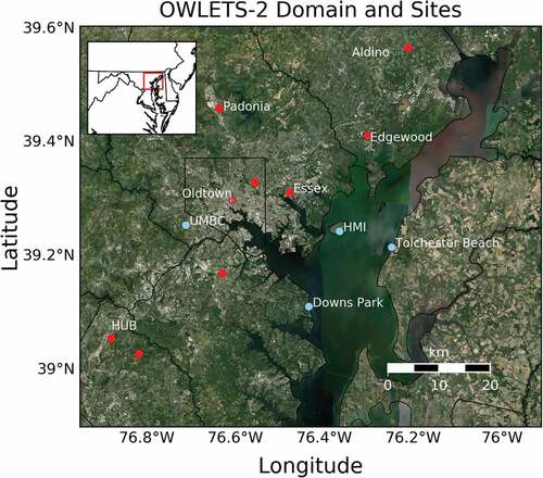
Hart-Miller Island (HMI) is a 1,100-acre island located approximately 22 km east of downtown Baltimore and roughly 3–5 km from the main Maryland shore (Figure 1). Two instrumented trailers with in-situ trace gas, meteorological and remote sensing measurements were sited on the southern shore of the island adjacent to preexisting island infrastructure on the lower portion of the island retaining dike (39.2420°N, 76.3626°W). These trailers were connected to the electrical grid. No gasoline generators were on site for campaign purposes. VOC canisters were placed on the ground approximately 10 m south of the instrumented trailers, with canister inlet approximately 1 m above ground level (AGL), approximately 5 m above the water level and approximately 5 m away from the water’s edge, with a prominent exposure to the NCB.

Figure 1. The OWLETS-2 experimental domain over the northern Chesapeake Bay. Red dots are ozone monitors within the state of Maryland ozone network. Blue dots show stationary collection sites established for the campaign. OWLETS-2 specific VOC collection was conducted at Hart Miller Island (HMI). Permanent VOC collection sites for the state of Maryland network were located at Howard University Beltsville (HUB) and Essex. A limited additional VOC dataset was available at Oldtown without collocated ozone (open red circle). The inset map provides a broader regional context.

Access to the island was only possible via boat. The ferrying boat docked at a location on the western side of the island 2 km away from the research site (39.2432°N, 76.3856 °W). Light duty vehicles transported personnel from the dock to the facility at approximately 0700 EDT and from the facility to the dock at approximately 1430 EDT. A barge dock located on the south shore of the island immediately adjacent the infrastructure powering the campaign site intermittently receives deliveries. However, no active docking of boats occurred, no barge deliveries were made, and no vessels were continuously moored, docked, or operated there during the campaign.

Measurements

An extensive suite of observation platforms building on measurement capabilities of OWLETS-2017 (Sullivan et al. 2019) were deployed to HMI to conduct over-water measurements downwind of the Baltimore urban plume. Aircraft complemented surface observations which were nested within the monitoring network operated by the state of Maryland. Due to logistics of operating on an island, non-continuous sampling (airplane, VOCs, etc.) targeted days of potential high ozone and/or fitting the conceptual model discussed in Dreessen et al. (2019). Instrumentation and data discussed are listed in Table 1.

Table 1. Instrumentation and data produced by location or platform used in this study.

Species	Location	Resolution	Total Samples (matching)	Instrument	Method	Notes
VOCs	Essex	1-hour	6080 (101)	Markes-Agilent Auto-GC	Preconcen trap/Thermal Desorber	2016–2018 (matching = HMI 2018 Samples)
		24-hour	45	Entech Canister; EnTech/Agilent GC/FID & MS	TO-12 (PAMS) GC-FID & TO-15 (GC-MS)	2016–2018
	Oldtown	24-hour	44	Entech Canister; EnTech/Agilent GC/FID & MS	TO-12 (PAMS) GC-FID & TO-15 (GC-MS)	2016–2018
	HU-Beltsville	3-hour	728 (6)	Entech Canister; EnTech/Agilent GC/FID & MS	TO-12 (PAMS) GC-FID & TO-15 (GC-MS)	2016–2018 (matching = June 19 & July 1, 2018)
		24-hour	46	Entech Canister; EnTech/Agilent GC/FID & MS	TO-12 (PAMS) GC-FID & TO-15 (GC-MS)	2016–2018
	HMI	3-hour	34	Entech Canister; EnTech/Agilent GC/FID & MS	TO-12 (PAMS) GC-FID & TO-15 (GC-MS)	2018: 10 days
	Airplane	2-minute	36	Entech Canister; EnTech/Agilent GC/FID & MS	TO-12 (PAMS) GC-FID & TO-15 (GC-MS)	7 flights (4 days)
NO	HMI	1-minute	May 24-August 1 (HMI VOC collection)	TECO 42C	Chemiluminescence	Entire 2018 Campaign
	Airplane	2-seconds	4 days	TECO 42C	Chemiluminescence	7 flights (4 days)
	Essex	Hourly	May 24-August 1 (HMI VOC collection)	Teledyne API 200 EU/501	Chemiluminescence	Entire 2018 Campaign
NO2	HMI	1-minute	same as NO	Los Gatos Research	Cavity Ring Down	Entire 2018 Campaign
	Airplane	2-seconds	same as NO	Los Gatos Research	Cavity Ring Down	7 flights (4 days)
	Essex	Hourly	same as NO	Teledyne Model T500 U	Cavity Attenuated Phase Shift Spectroscopy	Entire 2018 Campaign
NOy	HMI	1-minute	same as NO	TECO 42C	Chemiluminescence	Entire 2018 Campaign
	Airplane	2-seconds	same as NO	TECO 42C	Chemiluminescence	7 flights (4 days)
	Essex	Hourly	same as NO	Teledyne API 200 EU/501	Chemiluminescence	Entire 2018 Campaign
O3	HMI	1-minute	same as NO	TECO_49C	UV photometric	Entire 2018 Campaign
	Airplane	2-seconds	same as NO	TECO_49C	UV photometric	7 flights (4 days)

VOC collection and analysis

A total of 34 whole-air VOC canister samples were collected over 10 days at HMI. Seven flights over 4 days with a University of Maryland (UMD) aircraft collected an additional 36 samples. The VOC dataset included days both in excess and below the 70-ppb maximum daily 8-hour average ozone (MD8AO) at HMI (a NAAQS exceedance) and weekend and weekdays (Table 2). VOC samples at HMI were 3-hour collections using Entech 6 L canisters four times daily during intensive sampling days. Sampling canisters were lined with Silonite, an inert ceramic interior preventing deterioration of compounds within the air samples. Integrated samples were accomplished using Nutech 2701 programmable sampling timers, allowing regimented observations on specific days and times using a measured valve opening. A pressure gauge included as part of the Nutech timer assembly ensured proper negative pressure prior to canister use. Canisters and timers were waterproofed, and their inlets covered by metallic mesh to prevent contamination. Identical canisters without timers were used within the UMD Cessna aircraft. Aircraft samples were 2-minute duration.

Table 2. The number of VOC canister (Cans) samples by day and day of week (DOW) collected at HMI or by the University of Maryland (UMD) Cessna aircraft during the OWLETS-2 campaign. Maximum 8-hour ozone values were from HMI. An ‘E’ signifies a regulatory ozone exceedance occurred within the domain that day; HMI was not a regulatory site. Dashes (-) were days when the UMD aircraft did not fly in the experimental domain. The number of daily aircraft flights is given in parentheses. Holidays or days impacted by holidays are marked by superscripts(^H). Father’s Day, while not a federal holiday, sees increased boating activity and occurred on Sunday June 17, 2018. The July 4^th federal holiday impacted July 1 and 2.

Sample Date	HMI Cans	UMD Cans	DOW	Max 8-hour Ozone [ppbv]
2018-06-08	4	-	Friday	58
2018-06-17^H	4	6 (1)	Sunday	74 E
2018-06-18	4	12 (2)	Monday	61 E
2018-06-19	1	-	Tuesday	46
2018-06-24	3	-	Sunday	48
2018-06-29	4	9 (2)	Friday	79
2018-06-30	4	9 (2)	Saturday	85 E
2018-07-01^H	5	-	Sunday	79
2018-07-02^H	4	-	Monday	64 E
2018-07-05	1	-	Thursday	27

Sampling strategy at HMI used four 3-hour VOC canisters to cover the diurnal cycle, resulting in four 3-hour sample periods: 0600–0900, 0900–1200, 1200–1500, 1500–1800 LT. Two additional canisters sampled the 0600–0900 period during non-intensive days. One canister sampled the predawn chemical composition from 0300 to 0600 LT on July 1, 2018, during an extended high ozone period over the water (Table 2). The 3-hour sample procedure was optimized to avoid biased contributions from short-lived sporadic events such as occasional near-shore boat traffic adjacent to the site. VOC identification was accomplished with method TO-12 Photochemical Assessment Monitoring Station (PAMS) method, which uses Gas Chromatography with Flame Ionization Detector (GC-FID). Gas Chromatography with Mass Spectrometry (Method TO-15; GC-MS) measured air toxics (Table 1). EPA PAMS method employs a NIST certified standard containing the PAMS compounds of interest. The standard is supplied to the analysis lab by EPA every year. A predetermined standard curve of the target compounds is used to calculate specific PAMS compounds to prevent compound peak overlap.

Additional routine, EPA required VOC observations were available at Essex (39.3109°N, 76.4745°W), HUB (39.0553°N, 76.8786°W), and Oldtown (39.2977°N, 76.6046°W) sites in Maryland (Figure 1). A dataset of 24-hour canisters from June, July, and August 2016–2018 provided context for VOC concentrations at HMI. Collection of 24-hour VOCs was done at Essex and HUB according to a nationally consistent, EPA defined, preset one-in-six-day schedule. A limited additional 24-hour dataset of compounds cross listed as EPA Toxics and PAMS was collected at Oldtown. Additional 3-hour canisters were collected on a predefined one-in-three-day summer-only schedule at HUB. The Essex site also contained an automated gas chromatograph (Auto-GC), operational June to August annually, measuring hourly VOC concentrations for target EPA PAMS species (https://www3.epa.gov/ttnamti1/pamsmain.html). Throughout this study 3 and 1-hour datasets were matched with VOC collection times at HMI to provide simultaneous comparisons. Six 3-hour canisters at HUB overlapped with HMI canisters in OWLETS-2 while the Auto-GC at Essex provided a fully matched sample (Table 1).

Non-VOC trace gas and meteorology measurements

In-situ monitoring of meteorology and trace gasses occurred continuously for roughly the period of May 24 through July 31, 2018, without significant interruption, regardless of intensive coordinated measurements involving VOC canisters. Trace gas measurements of nitrogen compounds were conducted with a TECO 42C for (NO-NO_y), and LGR Cavity Ring Down for NO₂ on both HMI and the aircraft. Measurements at Essex were conducted via Teledyne API T500 U Cavity Attenuated Phase Shift (CAPS) for direct NO₂ measurements and the Teledyne API T200 U NO_y Chemiluminescence analyzer for NO and NO_y. Data resolution for the various platforms is provided in Table 1.

Results

Emissions

EPA 2017 NEI¹ and gridded emissions² provided context for observations. Gridded emissions were 12 km resolution and formatted for the Community Multiscale Air Quality (CMAQ) model by EPA based on the 2017 NEI. Sunday, June 18, and Friday, June 30, 2017 were of similar significance in 2018 (Father’s Day Sunday and the last Friday in June prior to the July 4^th holiday) and were meteorologically analogous (southwesterly surface winds, dry, and maximum temperatures of 92°F and 93°F respectively). Mean total VOC emissions (g s⁻¹) over the gridded domain on June 18, 2017, highlighted greater emissions along the interstate 95 corridor between Baltimore City and Washington D.C. (Figure 2a). A sharp spatial gradient was noted between Baltimore and the northern Chesapeake Bay with Essex in closer proximity to higher emission sources than HMI. Mean daily emission rate and total emissions, respectively, extracted from grids containing Essex and HMI were 21.0 g s⁻¹ and 1814 kg at Essex and 15.0 g s⁻¹ and 1300 kg at HMI on the representative Sunday. Relatively uniform VOC emissions existed across the Chesapeake Bay.

Figure 2. VOC emission from the 2017 National Emissions Inventory (NEI) for a representative weekday and weekend with similar meteorology. The 12 km grid of mean daily VOC emissions for (a) Father’s Day, Sunday, June 18, 2017, and (c) Friday, June 30, 2017, show the spatial distribution and differences between weekday and weekend. Essex and HMI are marked with points. Counties and cities referenced in the text are labeled. The diurnal distribution of total VOCs and toluene are given and (b) and (c) for their respective dates. Emissions were extracted from the respective 12 km grid in which HMI or Essex resided. Emissions are more prominent at Essex.

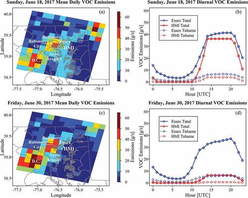
A diurnal comparison between land and water showed greater emissions persisted through the day at Essex (Figure 2b). Temporally, both sites followed a similar trend, with peak VOC emissions occurring from 14 to 20 UTC (10 am-4 pm LT). Emissions have some afternoon variability at Essex but were held constant at HMI. CMAQ speciates a select few VOCs within the model framework. Similar diurnal patterns were noted for toluene at both sites, with more toluene noted at Essex (318.6 kg) than at HMI (141.4 kg) through the entire period amounting to approximately 18% and 11% of total VOCs emitted, respectively (Figure 2b).

On Friday, June 30, 2017, greater VOC emissions were noted between Washington D.C. and Baltimore (Figure 2c) with fewer VOCs over the Chesapeake Bay. Mean daily emission rate and total emissions were 19.9 g s⁻¹ and 1716.0 kg at Essex and 2.7 g s⁻¹ and 235.4 kg at HMI, a much larger discrepancy between the two sites during the weekday. The dramatic reduction in total VOC emissions at HMI, most notable in the afternoon, was likely due to weekday-weekend differences in Chesapeake Bay usage (Figure 2d). 308.4 kg of toluene were emitted at Essex while only 25.8 kg were emitted at HMI, which were identical proportions as on Sunday June 18.

County level emissions were aggregated from Anne Arundel and Baltimore counties and Baltimore City, which lie directly west of Essex and HMI (Figure 2a,c). Anthropogenic area sources dominated total VOC emissions for all sectors in the 2017 NEI, followed by onroad sources (Table 3). Within the area sources solvents dominated, accounting for 77% of reported emissions within the sector. Hexane and toluene were specifically reported within the inventory. These species were overwhelmingly sourced from the onroad sector (Table 3). The “On-Road non-Diesel Light Duty Vehicles” category accounted for 89% of hexane emissions within the onroad sector.

Table 3. 2017 NEI and broken down by sector contribution to total VOCs, hexane, and toluene. Emissions were aggregated from Baltimore and Anne Arundel Counties and Baltimore City in Maryland. Values given are in tons with percentage contribution from each sector to the overall total provided in parentheses.

Tons (%)	VOC Emissions by Source Category
	Point	Area	Onroad	Nonroad	Event	Biogenic	Total
Total VOCs	977 (2.4)	16,147 (39.3)	6,809 (16.6)	3,804 (9.3)	42 (0.1)	13,287 (32.4)	41,066
Hexane	9.4 (3.7)	31.2 (12.3)	163.5 (64.7)	48.5 (19.2)	0 (0)	0 (0)	252.7
Toluene	5.9 (0.4)	358.4 (26.4)	654.5 (48.1)	340.3 (25.0)	0.4 (0)	0 (0)	1,359.4

Distribution of the 2017 NEI gridded NO_x was similar to VOCs. The mean daily NO_x emissions (g s⁻¹) over the domain on Sunday June 18, 2017, highlight the corridor between Baltimore and Washington DC along interstate 95, with a sharp spatial gradient toward the Chesapeake Bay (Figure 3a). Mean daily emission rate and total emission, respectively, were 14.2 g s⁻¹ and 1223 kg at Essex and 4.2 g s-1 and 366 kg at HMI. The NO_x diurnal pattern at HMI was notably delayed compared Essex and also to the HMI VOC diurnal pattern. However, the temporal pattern for both still peaked from 14–20 UTC (Figure 3b).

Figure 3. As in Figure 2, except for NO_x.

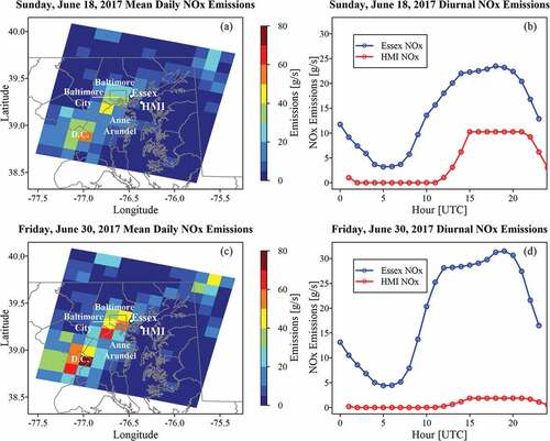
On Friday, June 30, 2017, greater NO_x was noted along the Washington D.C. to Baltimore corridor, as expected during a weekday (Figure 3c). However, a stronger disparity between the land and water cells at Essex and HMI was apparent. Mean daily emission rate and total emissions were 19.0 g s⁻¹ and 1643.5 kg at Essex and 0.8 g s⁻¹ and 68.0 kg at HMI. A delay in NO_x relative to Essex and VOCs was again noted at HMI (Figure 3d). Afternoon emissions were notably lower than the weekend, implying differing uses causing emission changes weekday to weekend. Aggregated county level emissions showed onroad NO_x sources dominant in the three county region (Table 4). Onroad, area, and point sources accounted for 90% of all NO_x within the inventory.

Table 4. As in Table 3, except for NO_x (NO₂ + NO) emissions.

Tons (%)	NOx Emissions by Source Category
	Point	Area	Onroad	Nonroad	Event	Biogenic	Total
Total NOx	5,691 (20%)	8,824 (30%)	12,845 (40%)	2,669 (10%)	3 (0%)	379 (0%)	30,411

Meteorology

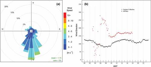
Winds were southerly and off the Chesapeake Bay during canister collection. During time periods of canister collection 73% of all wind observations had a direction between 140° and 225° (Figure 4a). All other directions had frequencies less than 5%. The winds between 0300 and 0600 (during a single canister 3-hour period) were the only significantly deviating from southerly. If this period were removed from consideration, southerly winds account for 86% of all observations during canister collection. A time series of the 10-minute binned average wind direction showed the evolution of wind direction through the canister sample periods (Figure 4b, red). Backing winds during the morning hours from 0600 LT through 1000 LT became steady from due south (180°) through the remainder of canister sampling periods. The HMI site otherwise had a southeasterly mean wind off the water throughout the campaign (Figure 4b, black). VOC samples were therefore primarily influenced by air with residence time over the NCB south of the island.

Figure 4. Wind rose during VOC canister collection periods (a) and mean diurnal time series of wind direction (b) over the entire campaign (black) and only during canister collection (red). The wind rose was built using one-minute resolution wind data. The time series was plotted using 10-minute average periods for smoothing.

Measurements of VOCs

Surface-based measurements

Analysis methods could identify 83 unique VOC species and total non-methane hydrocarbons (TNMHC). The top 20 compounds by median concentration amounted to 49% of the median TNMHC concentration (54.94 ppbv) measured at HMI, with the top ten compounds accounting for 41% (Table 5). Median TNMHC at HMI fell between the median 24-hour canister TNMHC concentrations at nearby Essex (36.9 ppbv), and HUB (89.8 ppbv). However, HMI had substantially more TNMHC than Essex (16.14 ppbv) or HUB (32.7 ppbv) using matching hours of VOC collection at HMI. The total of a subset of 54 of 56 VOC compounds (termed “PAMS” compounds with alpha and beta pinenes unavailable) deemed photochemically relevant for ozone production by EPA (US EPA 2004) was also statistically greater at HMI with median concentration of 24.58 ppbv. 24-hour canisters at Essex and HUB had median PAMS concentrations of 11.64 ppbv and 9.55 ppbv, and the Essex Auto-GC and HUB 3-hour canisters were 9.36 ppbv and 16.93 ppbv, respectively. Most of the difference in TNMHC and PAMS compounds between the two land sites and HMI occurred during daylight hours.

Table 5. Top 20 VOC species by median concentration (ppbv) over all canisters collected during the OWLETS-2 campaign on HMI, 2018. Statistics given are median (Med), mean, maximum (Max), minimum (Min), and standard deviation (Std) of each compound. Maximum Incremental Reactivity (MIR) taken from Carter (2010). Compounds in all caps were analyzed with the PAMS method. Title case compounds were from the TO-15 method.

Rank	VOC Name	Med	Mean	Max	Min	Std	MIR
		(ppbv)
1	Acetone	7.04	8.2	36.83	3.58	5.51	0.36
2	HEXANE	3.43	3.37	6.78	0.7	1.57	1.24
3	ISOPENTANE	2.7	4.55	27.46	0.57	4.96	1.45
4	ETHANE	2.23	2.69	5.89	0.78	1.24	0.28
5	CYCLOHEXANE	1.82	2.52	8.87	0.68	1.67	1.25
6	TOLUENE	1.35	1.27	2.44	0.27	0.64	4
7	3-METHYLHEXANE	1.06	1.22	3.37	0.23	0.78	1.61
8	PROPANE	1.05	1.18	2.37	0.55	0.45	0.49
9	ETHYNE	0.94	1.2	3.71	0.5	0.72	0.95
10	PENTANE	0.93	1.2	4.67	0.19	1	1.31
11	ETHENE	0.75	0.86	1.52	0.54	0.27	9
12	Chloromethane	0.64	0.64	0.79	0.54	0.06	0.038
13	2-METHYLHEXANE	0.61	0.69	1.86	0.12	0.45	1.19
14	Dichlorodifluoromethane	0.54	0.56	0.67	0.49	0.04	NA
15	2,3-DIMETHYLPENTANE	0.51	0.55	1.35	0.12	0.31	1.34
16	2-METHYLPENTANE	0.33	0.34	0.56	0.11	0.12	1.5
17	HEPTANE	0.32	0.39	1.07	0.07	0.27	1.07
18	3-METHYLPENTANE	0.31	0.31	0.47	0.1	0.09	1.8
19	BUTANE	0.25	0.33	1.64	0.03	0.29	1.15
20	Trichlorofluoromethane	0.25	0.26	0.32	0.23	0.02	NA

The largest measured VOC by mass at HMI was acetone, followed by several alkanes, toluene, ethyne, and ethene (Table 5). Mass differences between HMI and other sites were primarily confined to these compounds (Figure 5) with large differences apparent only 13 km apart between HMI and Essex. To contextualize these differences, concentrations of isopentane, cyclohexane, and hexane at HMI in 2018 were compared with all measurements at Essex between 2016 and 2018. The highest concentration of isopentane observed at Essex between 2016 and 2018 was 7.55 ppbv (Figure 5b). In contrast, 18% of the canisters at HMI observed concentrations of isopentane larger than this maximum value at Essex. A maximum 15.33 ppbv concentration of cyclohexane was measured at Essex during the same period, but no other sample exceeded 1.02 ppbv (Figure 5c). At HMI, all but two canisters exceeded 1.02 ppbv. The maximum concentration for hexane at Essex was 3.75 ppbv, with the next highest at 1.96 ppbv (Figure 5d). At HMI 76% of canisters sampled hexane greater than 1.96 ppbv. In contrast, there was a dearth of isoprene at HMI with 0.03 ppbv median concentration (Figure 5e). Biogenics were more prevalent at HUB, where isoprene median concentrations were 1.19 ppbv (24-hour canister) and 3.02 ppbv (3-hour canister time-matching dataset; Figure 5a). Essex was a suburban site adjacent the urbanized Baltimore City area, but median concentrations of isoprene at Essex were still over ten times larger than HMI at 0.36 ppbv (24-hour canister) and 0.51 ppbv (Auto-GC dataset). The character of VOCs at HMI compared to nearby land sites suggested unique source influences over the water during the intensive observation days.

Figure 5. VOC concentrations (ppbv) of (a) 55 VOC compounds (available PAMS compounds plus acetone) at four sites in Maryland, sorted by carbon number and concentrations distributions of isopentane (b), cyclohexane (c), hexane (d), and isoprene (e) at HMI and Essex. VOCs at Howard University Beltsville (HUB) and Essex were from 24-hour collection (HUB-24 hr: red; Essex-24 hr: blue) for June, July, and August 2016 – 2018. HUB 3-hour canisters (HUB-3 hr: orange) and hourly Auto-GC collection at Essex (Essex-AGC: light blue) were matched with VOC collection times at HMI for simultaneous data collection. Note the logarithmic vertical axis in (a). A few select species at HMI (green) dominate the concentrations at other collection sites in Maryland.

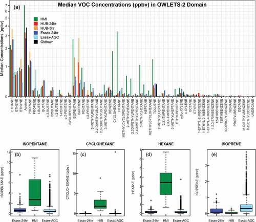
Though few species accounted for the total mass disparity between Essex and HMI, 28 of 53 PAMS compounds had greater median concentrations at HMI, 26 of which had relative differences at least double (100% greater) at HMI than Essex (Table 6). In this way, highly reactive species of low concentration, such 1-pentene, were identified as notably greater than at Essex. By percentage, compounds greater at HMI were dominated by C₅-C₉ species. Compounds lower at HMI were dominated by C₉+ species. Isoprene was among the lowest compounds at HMI compared to Essex. The Auto-GC at Essex did not measure acetone, but long-term canister datasets at Essex, HUB, and Oldtown (e.g., Figure 5a) suggested acetone concentrations 84%-116% higher at HMI than these other sites. Ethyne was 161.1% greater at HMI but was only significantly greater at HMI compared to simultaneous Essex Auto-GC measurements (Figure 5a). Similarly, species 41–53 in Table 6 were only sporadically detected at HMI resulting in 0 ppbv median concentration but were detected more frequently at Essex.

Table 6. A relative comparison of median PAMS VOCs (ppbv) measured at HMI and at the Essex Auto-GC. Relative differences, calculated by normalized differencing (% Diff), is the relative median concentration at HMI compared to Essex as a percentage. A − 100% indicates the median concentration at HMI was 0 ppbv. Compounds with a 0 ppbv median at Essex or not capable of being observed at either site were excluded.

Rank	VOC	HMI	Essex	% Diff
1	2,3DIMETHYLPENTANE	3.54	0.02	17,600
2	CYCLOHEXANE	10.95	0.14	7,721.4
3	HEXANE	20.57	0.95	2,065.3
4	STYRENE	0.38	0.02	1,800
5	3-METHYLHEXANE	7.45	0.52	1,332.7
6	2-METHYLHEXANE	4.26	0.37	1,051.4
7	1-PENTENE	0.85	0.12	608.3
8	ISOPENTANE	13.52	2.11	540.8
9	ETHYLBENZENE	1.55	0.27	474.1
10	HEPTANE	2.24	0.4	460
11	TOLUENE	9.41	1.98	375.3
12	METHYLCYCLOPENTANE	1.33	0.28	375
13	METHYLCYCLOHEXANE	1.04	0.24	333.3
14	PENTANE	4.66	1.17	298.3
15	3-METHYLPENTANE	1.88	0.58	224.1
16	2-METHYLPENTANE	2	0.7	185.7
17	124TMBENZENE	0.5	0.19	163.2
18	CYCLOPENTANE	0.47	0.18	161.1
19	ETHYNE	1.88	0.72	161.1
20	2,4DIMETHYLPENTANE	0.48	0.19	152.6
21	135TMBENZENE	0.2	0.08	150
22	DECANE	0.12	0.05	140
23	BENZENE	1.29	0.55	134.5
24	m&p-XYLENE	1.75	0.75	133.3
25	o-XYLENE	0.71	0.34	108.8
26	OCTANE	0.37	0.18	105.6
27	2,3-DIMETHYLBUTANE	0.48	0.34	41.2
28	ETHENE	1.5	1.29	16.3
29	PROPANE	3.16	3.19	−0.9
30	ISOBUTANE	0.6	0.62	−3.2
31	2,2-DIMETHYLBUTANE	0.16	0.17	−5.9
32	ETHANE	4.46	5.21	−14.4
33	3-METHYLHEPTANE	0.12	0.15	−20
34	1-BUTENE	0.58	0.8	−27.5
35	2-METHYLHEPTANE	0.11	0.16	−31.2
36	2,3,4-TMPENTANE	0.22	0.36	−38.9
37	BUTANE	1	1.69	−40.8
38	2,2,4TMPENTANE	0.7	1.21	−42.1
39	PROPENE	0.5	2.41	−79.3
40	ISOPRENE	0.14	2.55	−94.5
41	1-ETHYL-2-MBENZENE	0	0.07	−100
42	1-ETHYL-3-MBENZENE	0	0.01	−100
43	1,2,3-TRIMBENZENE	0	0.53	−100
44	c-2-BUTENE	0	0.15	−100
45	c-2-PENTENE	0	0.09	−100
46	ISOPROPYLBENZENE	0	0.03	−100
47	M-DIETHYLBENZENE	0	0.04	−100
48	NONANE	0	0.14	−100
49	P-DIETHYLBENZENE	0	0.05	−100
50	PROPYLBENZENE	0	0.06	−100
51	t-2-BUTENE	0	0.36	−100
52	t-2-PENTENE	0	0.15	−100
53	UNDECANE	0	0.1	−100

Aircraft measurements

The UMD plane collected 36 airborne VOC samples over water and land, both near and removed from HMI, and in both morning and afternoon flights at an average (median) altitude above ground level (AGL) of 495 m (336 m) overall, 457 m (325 m) over land and 549 m (341 m) over water. The lowest altitude of VOC collection over water occurred at 305 m AGL. Aircraft vertical profiles over HMI observed the top of the marine boundary layer (MBL) between 240 m and 365 m AGL depending on the day and time, indicating most VOC canisters were collected near or just above the marine boundary layer height. The geographic distribution of canisters was presented within the reactivity discussion in Figure 8c. Ethane, propane, ethene, ethyne, toluene, isopentane, pentane, and methylpentane isomers were similarly ranked within the top 20 compounds in the aircraft as at HMI (Table 7, left) though the distribution of the top 20 compounds was markedly different than at HMI (cf. Tables 3 and 7). Other VOCs were less prominent at HMI, including trimethylpentanes and propene. Hexane compounds prominent at HMI were scarcely measured by the aircraft. The median aircraft cyclohexane observation was 0.0 ppbv. Such disparity points to emissions at the marine surface.

Table 7. Top 20 individual VOC species by median concentration (ppbv) over all canisters collected during the OWLETS-2 campaign by the UMD aircraft over four days and seven flights. A total of 36 canisters were collected, 15 over the Chesapeake Bay. Statistics given are median (Med), mean, Maximum (Max), Minimum (Min), and Standard Deviation (Std) of each compound’s concentration. The TO-15 method was not available for the aircraft canisters. The left-hand side provides statistics for all aircraft samples. The right-hand side provides summary statistics for samples over the Chesapeake Bay only. Geographic distribution of samples is available in Figure 8c.

	All UMD Canister Samples (36 Canisters)						UMD Canister Samples over the Chesapeake Bay Only (15 Canisters)
Rank	VOC Name	Med	Mean	Max	Min	Std	VOC Name		Med	Mean	Max	Min	Std
1	ETHANE	2.09	2.11	5.13	0.72	1.14		ETHANE	1.44	1.81	5.13	0.92	1.10
2	PROPANE	0.77	0.86	3.41	0.31	0.63		PROPANE	0.52	0.76	3.41	0.37	0.73
3	ETHENE	0.30	0.37	1.02	0.23	0.20		ETHYNE	0.28	0.51	1.73	0.17	0.42
4	ETHYNE	0.28	0.47	1.73	0.06	0.40		ETHENE	0.28	0.35	1.02	0.24	0.19
5	TOLUENE	0.22	0.47	3.86	0.05	0.82		TOLUENE	0.19	0.48	3.86	0.08	0.92
6	BUTANE	0.17	0.34	1.96	0.06	0.41		BUTANE	0.14	0.29	1.96	0.08	0.47
7	ISOPENTANE	0.16	0.42	3.56	0.05	0.79		1-PENTENE	0.12	0.12	0.44	0.01	0.10
8	1-PENTENE	0.12	0.12	0.44	0.01	0.09		ISOPENTANE	0.11	0.39	3.56	0.05	0.87
9	2,2,4TMPENTANE	0.11	0.51	5.05	0.02	1.20		2,2,4TMPENTANE	0.11	0.51	5.05	0.05	1.23
10	ISOBUTANE	0.09	0.13	0.60	0.04	0.12		PROPENE	0.08	0.12	0.51	0.06	0.11
11	PROPENE	0.08	0.12	0.51	0.05	0.10		2,3,4-TMPENTANE	0.07	0.22	1.78	0.03	0.43
12	PENTANE	0.07	0.13	0.70	0.02	0.14		ISOBUTANE	0.07	0.11	0.60	0.05	0.14
13	2,3,4-TMPENTANE	0.07	0.25	1.98	0.01	0.50		PENTANE	0.07	0.14	0.70	0.03	0.17
14	CYCLOPENTANE	0.06	0.09	0.29	0.01	0.07		CYCLOPENTANE	0.05	0.09	0.29	0.01	0.09
15	3-METHYLHEXANE	0.05	0.07	0.40	0.01	0.08		3-METHYLHEXANE	0.05	0.08	0.40	0.01	0.11
16	1-BUTENE	0.05	0.07	0.42	0.01	0.09		2,3DIMETHYLPENTANE	0.03	0.14	1.27	0.02	0.31
17	2-METHYLPENTANE	0.04	0.07	0.50	0.00	0.10		1-BUTENE	0.03	0.06	0.32	0.01	0.08
18	2,3DIMETHYLPENTANE	0.04	0.15	1.27	0.00	0.30		2-METHYLPENTANE	0.03	0.07	0.50	0.01	0.12
19	BENZENE	0.03	0.06	0.40	0.02	0.08		2,4DIMETHYLPENTANE	0.02	0.11	1.07	0.01	0.26
20	3-METHYLPENTANE	0.03	0.08	0.59	0.01	0.12		BENZENE	0.02	0.05	0.40	0.02	0.10

Median concentrations of samples taken only over the Chesapeake Bay were nearly unchanged (Table 7, right), suggesting regional or terrestrial sources influencing the air over the water consistent with samples outside the marine boundary layer. Still, 3-methylhexane, ethyne, pentane, and toluene had higher average measurements over water. For example, 3-methylhexane was19% greater in average concentration in over-water canisters, indicating a possible origin within the marine airshed. These four compounds were the 7^th, 9^th, 10^th, and 6^th greatest compounds by concentration at HMI, respectively, and were 1333%, 161%, 298%, and 375% greater at HMI than at Essex, respectively, consistent with sources over the water influencing the marine layer.

Reactivity

Surface

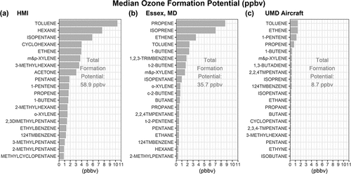
Ozone formation potential, the amount of ozone produced by a given VOC in the presence of NO_x, was calculated by multiplying specific VOC species concentrations by the Maximum Incremental Reactivity (MIR) provided by Carter (2010). Toluene, isopentane, hexane, cyclohexane, and ethene were the top five VOC compounds for ozone reactivity at HMI (Figure 6a). Acetone is not highly reactive nor typically considered in ozone production, but the high concentration at HMI raised its contribution among the top ten species. Many of the top 20 reactive compounds were within the top species by concentration and those of C₅ and greater dominate at HMI, with many isomers of hexane and heptane. With the noted exception of benzene, BTEX compounds (benzene, toluene, ethylbenzene, xylenes) were also among the top reactive compounds. 1-pentene had a relatively small concentration, but the relative difference to Essex was large and the species fell in the top ten ozone formation potential. Toluene had the highest ozone formation potential at HMI with a concentration nearly four times greater than Essex. Reactivity at Essex was dominated by propene and isoprene (Figure 6b). Propene has several possible sources including diesel fuel, where isoprene is biogenic. Only ethene and toluene were similarly in the top five compounds at HMI and Essex. Despite their 13 km proximity, distinct chemical makeups drove ozone formation between the two sites.

Figure 6. Calculations of ozone formation potential using maximum incremental reactivity (MIR) for the top 20 ranked VOC species based on median VOC concentration at (a) HMI, (b) simultaneous observation at the Essex Auto-GC, and (c) UMD aircraft from samples taken over the Chesapeake Bay only. MIR calculations based on Carter (2010). Total ozone formation potential of all species was also supplied for each dataset. Acetone was not available at Essex or in the aircraft data for simultaneous comparison.

Aircraft

Top ozone formation potential VOCs in aircraft measurements taken over the Chesapeake Bay were toluene, ethene and 1-pentene (Figure 6c). These three and several other VOCs were similarly noted within top ranking reactive VOCs at HMI, suggesting sources influencing a wider region or vertically deeper layer over water for some VOCs. Cyclohexane and hexane were not among the compounds with high ozone formation potential in the aloft dataset. Consistent with greater number of PAMS species at HMI, ozone formation potential at the NCB surface remained greater than air just 300–400 m above the water surface and adjacent land sites on sample days.

Diurnal pattern

The diurnal variation of VOC concentrations at HMI was opposite that of typical land-based VOCs in Maryland. VOC concentrations at HUB and Essex land-based sites were greatest in the overnight and early morning hours, likely due to lower reactivity, boundary layer depth, and introduction of daily emissions during the morning rush hour (Figure 7a). Long-term datasets at Essex (blue) and HUB (red) showed decreasing PAMS VOC concentrations through midday (Figure 7a, “Full”). In contrast, VOC concentrations on sampled days at HMI were greater than nearby sites and peaked during the midday hours (green, Figure 7a).

Figure 7. (a) Diurnal VOC concentrations of the EPA PAMS VOC subgroup at HMI (bold green), Howard University-Beltsville (HUB, bold red) and Essex (bold blue) and select species at HMI (black dashed/dotted lines). (b) Diurnal concentrations of median NO_y and NO_z at HMI (oranges) and Essex (blues). Full data sets use June 1 – July 10, 2018, except diurnal VOC cycles at HUB which were created from 3-hour canisters collected every one-in-three-days and at Essex using hourly observations from the Automated Gas Chromatograph unit, in June, July, and August, 2016–2018. Match data sets only use simultaneous observation times with VOC canisters on HMI in 2018. HMI VOC concentrations increased diurnally and were greater compared to the other sites. Range on (b) was limited to 12 ppbv for clarity at lower concentrations. The peak NO_y on Match days reached 19.40 ppbv at 0300 LT at Essex.

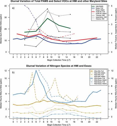
Simultaneous VOC measurements from Essex and HUB as at HMI (Figure 7a, dashed lines, “Match”) also revealed persistently greater VOCs at HMI diurnally. The top three VOCs for ozone potential at HMI (Figure 7a: toluene, solid black line; isopentane, dashed line; hexane, dotted line) exhibited similar behavior as total VOCs, increasing midday. These species were also among the top mass contributors at HMI and thus account for much of the diurnally increasing mass at HMI. Acetone, in contrast, had peak concentration at HMI overnight with 10.14 ppbv in the 0300 canister, 22% higher than the next highest midday (1200) canister concentration (8.31 ppbv) suggesting a different source.

The early morning (0300–0600 LT) canister at HMI in Figure 7a sampled the pre-dawn morning of July 1, after an ozone exceedance at HMI on June 30 and preceding an additional exceedance on July 1. This sample measured the third lowest PAMS VOC subset concentration of any canister collected. The two lowest PAMS concentrations were both sampled in the 0600–0900 LT period, with clean Atlantic Ocean air on July 5 (southeast trajectories) and a post frontal airmass June 29. While the predawn sample was a single canister, low concentrations within the 0600–0900 LT period were observed with multiple canisters supporting the assertion that VOC concentrations were lower nocturnally over the water on sample days of OWLETS-2.

Measured nitrogen compounds

Hourly averaged total reactive nitrogen (NO_y), NO_x (NO_x = NO₂ + NO) and reservoir species (NO_z = NO_y - NO_x) were available at HMI and Essex. HMI lacked the morning NO_y diurnal peak at Essex (“Full” Figure 7b) and reached a lower maximum NO_y concentration two hours later. The two sites had similar median NO_y concentrations during a midday period (~1000–1400 LT), but thereafter NO_y continued to decrease at HMI while it stabilized at Essex. Average observations of NO_y between June 1 and July 10, 2018, were 6.88 ppbv and 4.73 ppbv at Essex and HMI respectively, and 0.17 ppbv and 1.59 ppbv for NO_z, respectively.

NO_y and NO_z during VOC canister collection periods had mean concentrations of 8.22 ppbv and 0.85 ppbv at Essex, and 6.54 ppbv and 2.39 ppbv at HMI, respectively (“Match” Figure 7b). HMI showed a modified diurnal pattern (dotted lines Figure 7b) where median NO_y initially greater at Essex was surpassed by HMI after 0900 LT through 1500 LT with a noteworthy peak in NO_y at HMI at 1100 LT. The local peak of NO_y at HMI in the 0800–1200 LT period coincided with VOC increases at HMI. NO_z was always higher at HMI, peaking at 1400 LT, later and greater than the campaign median.

Weekday to weekend comparison

Weekend (Saturday and Sunday) concentrations were greater than weekday (Monday through Friday). The mean TNMHC concentration was 60.7 ppbv and 57.2 ppbv on the weekend and weekday respectively, over all measured hours, but failed significance (α = 0.05) using the Wilcoxon-Ranked Sum test for non-normal distributions. Significance was noted, however, comparing only the 0600 LT canisters with mean weekend and weekday TNMHC concentrations of 53.8 ppbv and 40.0 ppbv, respectively. Few VOC observations and some weekday periods impacted by altered holiday activity may have trended sampled weekdays toward the weekend profile and added uncertainty to VOC comparisons. However, NO_x concentrations at HMI were significantly greater on weekends based on observations from June through July, 2018. Mean weekday NO_x was 2.5 ppbv while weekend NO_x was 2.9 ppbv.

Ozone production efficiency

Ozone production efficiency (P(O₃)) in both HMI and aircraft VOC samples was assessed with a box model. The box model configuration included the Regional Atmospheric Chemistry Mechanism Version 2 (RACM2; Goliff, Stockwell, and Lawson 2013), with FACSIMILE software package (UES Software Inc.) to run the box model. The model was constrained with long-lived inorganic and organic compounds and measured meteorological parameters such as temperature, pressure, and relative humidity at HMI and along the aircraft flight track. Photolysis frequencies (J values) were calculated and scaled to measured solar radiation, with 34 and 35 VOC canister samples used in the model at HMI and aircraft, respectively. Model output included OH, HO₂, RO₂ and other reactive intermediates.

The net production of ozone at any given instance was the sum of ozone production minus ozone loss (1). Production and loss of ozone were driven in the model by equations (2) and (3), respectively. Net P(O₃) was a function of NO_x and VOCs (4) while the sensitivity of ozone production was determined by the indicator L_N/Q according to equation (5) where, L_N was the radical loss due to NO_x and Q was the total primary radical production, such that L_N/Q was essentially the fraction of radical loss due to NO_x. As such when L_N/Q > 0.5, P(O₃) was VOC-sensitive and with L_N/Q < 0.5, P(O₃) was NO_x-sensitive (Kleinman et al. 2001). Oxidized VOCs (OVOCs) also include other unmeasured but calculated OVOC species in the model besides measured acetone. Ozone production rates in the box model were instantaneous.

(1) $\mathrm{P}\left({\mathrm{O}}_3\right):\mathrm{P}{\left({\mathrm{O}}_3\right)}_{\mathrm{n}\mathrm{e}\mathrm{t}}=\mathrm{P}\left({\mathrm{O}}_3\right)-\mathrm{L}\left({\mathrm{O}}_3\right)$(1)

(2) $\mathrm{P}\left({\mathrm{O}}_3\right)={\mathrm{k}}_{\mathrm{N}\mathrm{O}+\mathrm{H}\mathrm{O}2}\left[\mathrm{N}\mathrm{O}\right]\left[\mathrm{H}{\mathrm{O}}_2\right]+{\sum }_{\mathrm{i}}{\mathrm{k}}_{\mathrm{N}\mathrm{O}+\mathrm{R}\mathrm{O}2\mathrm{i}}\left[\mathrm{N}\mathrm{O}\right]\left[\mathrm{R}{\mathrm{O}}_{2\mathrm{i}}\right]$(2)

(3) $\mathrm{L}\left({\mathrm{O}}_3\right)={\mathrm{k}}_{\mathrm{O}1\mathrm{D}+\mathrm{H}2\mathrm{O}}\left[\mathrm{O}{(}^1\mathrm{D}\right)\left]\left[{\mathrm{H}}_2\mathrm{O}\right]+{\mathrm{k}}_{HO2+\mathrm{O}3}\left[\mathrm{O}3\right]\right[H{O}_2\left]\text{break}+{\mathrm{k}}_{OH+\mathrm{O}3}\right[{\mathrm{O}}_3\left]\left[OH\right]+{\mathrm{k}}_{OH+NO2+\mathrm{M}}\left[OH\right]\right[N{O}_2]\left[\mathrm{M}\right]$(3)

(4) $\mathrm{P}\left({\mathrm{O}}_3\right)=\mathrm{K}{\mathrm{Q}}^{\mathrm{C}1}{\left[\mathrm{N}{\mathrm{O}}_{\mathrm{x}}\right]}^{\mathrm{C}2}{\left[\mathrm{V}\mathrm{O}\mathrm{C}\right]}^{\mathrm{C}3}$(4)

where K is the rate constant, and C1, C2, and C3 are constants for a specific LN/Q according to Kleinman (2005):

$\mathrm{C}1=\mathrm{d}\mathrm{l}\mathrm{n}\mathrm{P}\left({\mathrm{O}}_3\right)/\mathrm{d}\mathrm{l}\mathrm{n}\mathrm{Q},$

$\mathrm{C}2=\mathrm{d}\mathrm{l}\mathrm{n}\mathrm{P}\left({\mathrm{O}}_3\right)/\mathrm{d}\mathrm{l}\mathrm{n}\left[\mathrm{N}{\mathrm{O}}_{\mathrm{x}}\right]$, and

$\mathrm{C}3=\mathrm{d}\mathrm{l}\mathrm{n}\mathrm{P}\left({\mathrm{O}}_3\right)/\mathrm{d}\mathrm{l}\mathrm{n}\left[\mathrm{V}\mathrm{O}\mathrm{C}\right].$

(5) $\frac{dlnP\left(O3\right)}{dln\left[NOx\right]}=\frac{1-3/2L_N/Q}{1-1/2L_N/Q}\mathrm{a}\mathrm{n}\mathrm{d}\frac{dlnP\left(O3\right)}{dln\left[VOC\right]}=\frac{1/2L_N/Q}{1-1/2L_N/Q}$(5)

Surface

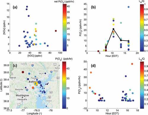
OH reactivity at HMI averaged 9.7 s⁻¹ (Table 8) and TNMHC and Oxidized VOCs (OVOCs) contributed significantly to OH reactivity. Net P(O₃) was simulated above 15 ppbv hr⁻¹ as VOC concentrations increased above 40 ppbv (Figure 8a). A few instances with NO_x above 10 ppbv had low P(O₃) due to relatively low VOC concentrations. In contrast, P(O₃) of 42 ppb hr⁻¹ was predicted with NO_x of ~ 6 ppbv and VOCs above 90 ppbv, the highest concentration of VOCs within the box model. Average P(O₃) mimicked VOC concentrations diurnally and was greatest during the mid-morning from 0900–1200 LT (Figure 8b) but with instances where P(O₃) was sustained above 25 ppbv hr⁻¹ through the afternoon. The largest P(O₃) was on Sunday June 17, 2018, during the late afternoon canister (1500–1800 LT). The canister with highest P(O₃) for the 1200–1500 LT period was also a Sunday, June 24, 2018 (Figure S1). Generally, the model indicated increasing NO_x sensitivity as L_N/Q became lower through the day.

Table 8. OH Reactivity from various precursors from the box model runs. Mean [median] total reactivity is given as s ⁻¹, all other values are percentage contribution of the modeled species. Oxidized VOCs (OVOCs) were modeled since few OVOC observations were available. Alkanes, alkenes, and isoprene & terpenes (right side) were sub-groups of the Non-Methane Hydrocarbons (NMHC) category.

	Mean [median] OH Reactivity (s^−1)	NOx	CO	Other	OVOC	NMHC	Alkanes	Alkenes	Aromatics	Isoprene & Terpenes
HMI	9.7 [8.8]	9	9	3	44	35	63	23	11	3
Aircraft	7.1 [4.8]	9	14	7	44	25	42	27	6	25

Figure 8. (a) Scatter plot of ozone production efficiency (P(O₃), (ppb hr ⁻¹)) at HMI for all 34 canisters within the box model as function of VOC and NO_x concentrations (ppbv). (b) P(O₃) of individual canisters (dots) by time of day (centered in 3-hour time bins), colored by NO_x sensitivity at HMI. The black line indicated the average P(O₃) for each period. L_N/Q > 0.5 is VOC sensitive while LN/Q < 0.5 is NO_x sensitive. The spatial distribution of P(O₃) from 35 UMD aircraft VOC canister samples over the OWLETS-2 domain is given in (c) with the temporal distribution of P(O₃) and L_N/Q from the aircraft samples in (d). Circle size in (c) represents total VOC concentrations with the minimum value of 4.2 ppbv and a maximum value of 99.4 ppbv.

Formaldehyde and acetaldehyde are two important chemical species in urban areas not directly measured by the TO-15 or PAMS methods. These species are resultant products of photochemical oxidation and may contribute to OH reactivity significantly. The box model predicted mean concentrations of 6.4 ppbv for formaldehyde and 3.6 ppbv for acetaldehyde, resulting in OH reactivity values of 1.30 s⁻¹ equally for both compounds. These compounds accounted for about two thirds of the OH reactivity from oxygenated volatile organic compounds (OVOCs), with each contributing 15% to the total OH reactivity at HMI.

Aloft

In the aircraft, OH reactivity was 7.1 s⁻¹, lower than at HMI. TNMHC and Oxidized VOCs (OVOCs) again contributed significantly to OH reactivity (Table 8), however, aloft, OH reactivity had larger contribution from isoprene and terpenes than at HMI, where alkanes dominated OH reactivity. P(O₃) aloft was greatest near the Baltimore urban area emission sources while over the Chesapeake Bay production was comparatively slow (Figure 8c). Four aircraft samples simulated P(O₃) above 15 ppbv hr⁻¹ but were all located over land. In fact, all samples located over the Chesapeake Bay had P(O₃) ~ 5 ppbv hr⁻¹ or less with lower VOC concentrations than near Baltimore. Morning and afternoon flights showed a combination of both NO_x and VOC sensitivity as well as variable P(O₃) (Figure 8d). However, the lowest afternoon P(O₃) and greatest NO_x sensitivity was almost solely found over the NCB (c.f. 8c & 8d).

Chemical regime

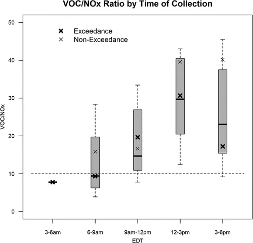
Mean NO_x was calculated in three-hour bins matching VOC collection periods and the VOC/NO_x ratio at HMI was calculated as a function of time of day (Figure 9). Dodge (1977) suggested a ratio of 8:1 as the transition of ozone sensitivity between NO_x and VOCs. However, this ratio is known to change throughout the day, by location, and by the mix of VOCs present. Box modeling of VOCs at the HMI surface site indicated a ratio of approximately 10:1 for this transition (Figure S2), similar to the suggested EPA ratio (Wolff and Korsog 1992). The VOC/NO_x ratio at HMI indicated increasing sensitivity of ozone to NO_x and a transition from VOC to NO_x sensitive regime on sample days (Figure 9). Comparatively, the ratio was substantially lower on ozone exceedance day afternoons due to both more NO_x and lower VOCs compared to non-exceeding days.

Figure 9. Box plot distributions of total non-methane hydrocarbon (TNMHC) over Nitrogen Oxides ratios (VOC/NO_x) for each time bin of canister collection at HMI. The dashed line at a ratio of ten divides ozone production chemical regimes. Ratios lower than 10 indicate ozone production sensitive to VOC concentrations. Ratios greater than 10 indicate ozone production sensitive to NO_x. Greater NO_x sensitivity was experienced in the afternoon with a transition from VOC limited morning conditions. Box plots show median, interquartile range, and extrema. Bold “x” are ozone exceedance day averages for that time bin while thin “x” are non-exceedance days.

Discussion

Accounting for observed land-water VOC disparity

The 2017 NEI showed VOC emissions were lower at HMI than at Essex and substantially lower at HMI on weekdays. Lower emissions suggested lower concentrations may be expected at HMI in the OWLETS-2 dataset. However, VOC PAMS species concentrations were two to three times greater at HMI than at Essex, despite their 13 km proximity, with greater total VOCs present at HMI as well. Similarly, despite weekend total NO_x emissions at HMI only 4% to that observed at Essex, midday and early afternoon NO_y concentrations were comparable between the two sites (Figure 7b).

The dichotomy of greater concentrations with lower emissions suggested boundary layer dynamics, inventory error, or a combination of both. Boundary layer depth over water is shallow and has been observed to be around 500 m during the afternoon over the Chesapeake Bay (Caicedo et al. 2021) with weak vertical mixing compared to land. Even minor surface emissions may maintain large concentrations in these conditions. Temporally, the largest NEI emissions at HMI occurred in the afternoon, consistent with peak observed concentrations at that time. Relatively uniform average VOC emissions occurred across the Chesapeake Bay (Figure 2a), such that southerly transport would produce the results seen here. By comparison, increased vertical mixing at Essex as VOC emissions reached their peak mitigated surface concentrations there. Conversely, minimal vertical mixing at Essex in the morning created a maximum in VOC concentrations before mixing out in the afternoon. The morning land scenario may act as a proxy to peak afternoon concentrations over water where mixing heights remained low even as VOC emissions at HMI peaked to rates similar to weekday mornings at Essex. The low mixing heights explanation would highlight the importance of even relatively small surface emissions over a shallow depth on the water. Alternatively, it also remained possible the NEI did not reflect sufficient VOC (or NO_x) emissions at the water site or that in comparisons, the Essex site may not have adequately captured or represented emissions from Baltimore and/or the ports, which may influence HMI but not necessarily Essex.

Sourcing excess VOCs at HMI

Many compounds comprising the greater VOC concentrations at HMI were identified as components of gasoline vapor. Cyclohexane had the second largest concentration compared to Essex, while heptane (ranked 10^th) and toluene (ranked 11^th) also had abundant concentrations compared to Essex. Toluene, heptane, and cyclohexane were identified as most abundant in gasoline vapor by Chin and Batterman (2012). The prominence of lighter compounds in gasoline including butane, isobutane, pentane, and isopentane have been noted elsewhere (Conner, Lonneman, and Seila 1995; Doskey, Porter, and Scheff 1992; Na et al. 2004), however reformulated gasoline contains heavier hydrocarbons to reduce emissions which contribute to ozone formation (US EPA 2015b). Additives such as toluene and 2,2,4-trimethylpentane (isooctane) decrease evaporative emissions by decreasing the Reid Vapor Pressure (RVP) while maintaining octane rating (da Silva et al. 2005). The EPA required reformulated gasoline with low RVP in the state of Maryland during the OWLETS-2 study period (https://www.epa.gov/gasoline-standards/reformulated-gasoline). California reformulated gasoline was comprised of toluene, cyclohexane, methylcyclohexane, heptane, and 2-methylpentane (Harley, Coulter-Burke, and Yeung 2000), which were compounds observed at HMI in high concentrations. Isopentane, toluene, butane, 2 and 3-methylpentane, hexane, cyclohexane and pentane comprised approximately half the contribution to a composite profile made of gasoline headspace vapor and diurnal gasoline permeation and evaporative emissions within EPA SPECIATE.³ Substantial reductions in benzene within gasoline likely accounted for the relatively low benzene compared to other compounds noted in the OWLETS-2 study (EPA 2016) though benzene concentrations at HMI were still double to that at Essex.

Both 2 and 3-methylpentane were used to identify and distinguish gasoline combustion emissions from fugitive emissions (Rubin et al. 2006). Rubin et al. found 2 and 3-methylpentane to be among the most abundant compounds in liquid gasoline, headspace vapors, and tunnel emissions, but noted that strongly enhanced isopentane to methylpentane was indicative of headspace vapors. In that study, isopentane was roughly a factor of 7–10 greater than methylpentanes in headspace vapors but was ~2–4 times greater in tunnel emissions. At HMI, linear fits of isopentane and 2 and 3-methylpentane had ratios of 11.3 and 12.8 (R² <0.08). The median 2 and 3-methypentane to isopentane concentration ratios were 8.1 and 8.6. These ratios indicated gasoline headspace vapors, though other sources cannot be ruled out. For example, methylhexane was identified as evaporative emissions from oil and condensate tanks (Hendler et al. 2009) but also as a non-trivial component of non-road, 2-stroke engine exhaust (Reichle et al. 2015) while 2,3-dimethylpentane has been observed in mobile emissions (Sagebiel et al. 1996).

Gasoline vapor also appeared to be primarily responsible for elevated hexane concentrations. Hexane was found in about 10% of household products in Korea, such as air freshener, disinfectant, furniture polish, and household sealants (Kwon et al. 2007) and has also been reported as a solvent to extract edible oils from seed and vegetable crops (e.g., soybeans, peanuts, corn), solvents for glues (rubber cement, adhesives), varnishes, and inks and as a cleaning agent (degreaser) in the printing industry (US EPA 2000). MDE permit-to-operate records include many hexane point sources in southern Baltimore City associated with gasoline storage facilities as the only significant hexane point sources in the study domain. However, mobile sources accounted for nearly 65% of hexane emissions in the 2017 NEI, of which nearly 90% was from light-duty non-diesel vehicles. Furthermore, hexane was primarily found in unburned whole gasoline from tailpipes or head space vapors in Lough et al. (2005). The amount of hexane and compounds such as 2,2,4-trimethylpentane was dependent on the seasonal mixture of gasoline. It was therefore likely most of VOC mass at HMI was reformulated “summer” gasoline vapor. This finding was largely consistent with findings by Henry (2013) who looked at coastal monitors in New England.

Not all the compound differences to nearby Essex were readily explained by evaporated gasoline. For example, styrene was noted as a minor component in vehicle emissions, but it was enhanced by nearby industrial emissions (Jobson et al. 2004), and previous studies have noted styrene as a major industrial chemical (Fu and Alexander 1992). Liu et al. (2008) identified emissions sources associated with compounds in abundance at HMI, many which were classified in oil or chemical refining (methylcyclohexane, hexane, and styrene), as well as diesel and gasoline exhaust and evaporation. 1-pentene was relatively abundant at HMI and may be found as a minor component of gasoline, in jet fuel, open burning, landfills, and has been noted in asphalt tar kettles (US EPA 1990), but also has marine biogenic sources (Tripathi et al. 2020).

Ratios of compounds are useful for distinguishing between sources. A ratio of 1-butene to 1-pentene was reported as ~1–3.75 for vehicular exhaust (Jobson et al. 2004). The ratio from HMI canisters was 0.26, with considerable scatter (R² = 0.01), suggestive of a non-exhaust source. A ratio of styrene to 1,3,5-trimethylbenzene of approximately 0.7–0.8 corresponds to vehicular exhaust. At HMI the ratio was 0.8 (R² = 0.07), suggestive of exhaust. Notwithstanding evaporated gasoline, industry can impact cyclohexane concentrations (Jobson et al. 2004). The ratio of cyclohexane to heptane was 0.47 (R² = 0.01), in good agreement with a ratio of 0.43 expected from vehicular exhaust. A hexane to 2-methylpentane ratio of 0.52 would suggest vehicular exhaust, but this ratio was 7.42 with R² = 0.30 at HMI, significantly higher due to enhanced hexane concentrations, implying a non-exhaust source. Considerable scatter and poor fit of many ratios make hard conclusions premature, with further investigation needed to distinguish a mix of sources likely present.

Acknowledging noteworthy uncertainty, given HMI’s location, dominant southerly wind off the water, and VOCs indicating evaporative and exhaust emissions, abundant VOCs were likely sourced from marine traffic. For example, ∼50% of VOC mass in tailpipe emissions consists of unburned gasoline in on-road vehicles (Leppard et al. 1992). Given the lack of catalytic exhaust conversion in most boats, this could be an underestimation for 4-cycle and 2-cycle marine engines. A study prior to the prominence of catalytic converters may more aptly represent boating emissions. Furthermore, the 2017 NEI apportioned 64.7% of hexane to the onroad sector suggesting gasoline engines account for hexane emissions. Four-stroke engines over water use similar gasoline as the onroad sector. Additionally, boat operational efficiency (running rich) and/or gasoline vapor venting from boats (such as after fueling) could also explain gasoline vapor (US EPA 2000). The diurnal increase in total VOCs at HMI would be consistent with increased volatization of petrochemicals and increased diurnal boating activity on the NCB. Increased VOC emissions over the NCB in the NEI on weekends (Figure 2a,b) likely reflects weekend boat usage.

Significance of land-water VOC disparity

The differing distributions and concentrations of VOCs at HMI compared to Essex showed disparate source impacts at HMI and Essex causing ozone curtailment to be dependent on location, even within 13 km proximity. Anthropogenic VOCs dominated at HMI, while isoprene, a biogenic compound, dominated at Essex. Alkanes at HMI had high ozone formation potential, with alkenes such as 1-pentene, ethene, and aromatic BTEX compounds also dominant. Isoprene was scarce at HMI. The aircraft measured much smaller concentrations than at HMI with noted absences of hexane, cyclohexane, and isopentane. Except for toluene and ethene, ranking of ozone formation potential was also different. Given the distribution of dominant VOCs across the land-water interface, curtailment strategy approaches may be different.

The enhanced VOC concentrations in the afternoon at HMI created an intensely NO_x sensitive environment over the water. While this meant reductions in NO_x would increasingly be effective at further ozone curtailment, it also meant ozone may respond quickly with episodically sufficient NO_x. For example, on Sunday, June 17, 2018 (Father’s Day in the US; A heavy boating day over the Chesapeake Bay) sufficient NO_x and the most abundant VOC concentration of the campaign produced P(O₃) of 42 ppbv hr⁻¹ at HMI, the highest P(O₃) of all canisters. Apart from the June 17 case, four other instances of P(O₃) > 25 ppbv hr⁻¹ occurred at HMI. These were specific events where more abundant sources of NO_x (or sources with more abundant NO_x) increased P(O₃) and pushed ozone above the NAAQS.

Despite the high concentration of VOCs, the average production rate of ozone was slow at HMI. P(O₃) in most canisters at HMI and ~300 m over the NCB in the aircraft was less than 10 ppbv hr⁻¹. VOC emissions in the NEI were larger than NO_x emissions at HMI, particularly during the weekend (c.f. Figures 2 and 3), causing or reinforcing the NO_x sensitive regime. The observed VOC/NO_x ratio showed increasing NO_x sensitivity diurnally over the water as well, suggesting the VOC source was not a sufficient NO_x source. Alternatively, it may be posed that NO_x became a component of NO_z in the VOC-rich air. In any event, typical conditions produced ozone slowly. Box modeling of aircraft measurements over land, in contrast, produced intense OH reactivity (>30 s⁻¹; not shown) and P(O₃) greater than 30 ppb hr⁻¹ near Baltimore sources. Thus, the air at HMI was typically aged based on the amount of NO_z and reduced P(O₃). Ozone production calculations were instantaneous and airmass history nor transport trajectories were included in this analysis. In circumstances with ozone above the NAAQS but reduced P(O₃), ozone at HMI would have been due to transport, not local production. Even still, it was clear that with sufficient NO_x at HMI, extremely rapid local production was possible. As such, continuing to mitigate NO_x and VOCs over the marine environment may act as curtailment strategy, with the data suggesting boats as the primary source.

Greater VOC concentrations at HMI than land sites may explain the greater concentration of reservoir species (NO_z) compared to Essex since VOCs facilitate products such as Peroxyacyl Nitrates (PAN). The NEI had little if any VOC emissions at night over the water. Therefore, reactivity may also explain oxidized VOC abundance (e.g., acetone), and be consistent with reduced overall VOC concentrations overnight. Acetone, in contrast with many VOC species, was greatest overnight at HMI, observing 10.14 ppbv in the 0300–0600 LT canister, 22% higher than the next highest midday (1200–1500 LT) canister concentration (8.31 ppbv). NO_x emissions were delayed at HMI compared to Essex in the NEI. The delay in ozone production at HMI compared to land sites noted by Dreessen et al. (2019) could be explained by this, though the proposed delay in NO_z dissociation from lagging temperature over the water remained plausible. Though why the morning NO_x emission increases were delayed more than VOC emissions at HMI in the inventory was not known. NO_z was found to be higher overnight prior to exceedance events during OWLETS-2, consistent with acetone observations. The over water air was thereby acting as a near-surface precursor reservoir supportive of ozone NAAQS exceedances the following day. As such, a reduction in VOC concentrations may act to reduce the carry-over of ozone precursors day-to-day that may subsequently impact the local region or be transported downstream.

Ozone formation is dependent upon NO_x availability but controlled by VOCs. Quicker ozone development leads to more time near or above the 70 ppbv NAAQS, increasing the likelihood of an 8-hour average exceedance. Even as NO_x can control total ozone development, VOCs may control the likelihood of an exceedance event by increasing the number of hours maximum ozone potential is reached. While widespread regional NO_x reductions reduced the regional ozone load, localized urban, facility, or boat exhaust plumes poorly dispersed due to proximity to water may achieve ozone rates that lead to exceedances of the ozone NAAQS when these plumes impact regulatory monitors.

Abundant VOCs over the marine environment also has implications for fine particulate matter policy. Reduction of VOCs could reduce secondary aerosol formation. Though Baltimore is in attainment for fine particles, reductions in VOCs may offer co-benefits of reducing ozone over the water and transported downstream while reducing fine particle formation to ensure continued compliance, particularly if a lower fine particle NAAQS was adopted.

Conclusion

TNMHC and PAMS subgroup VOC concentrations at HMI over the Chesapeake Bay were 2.1 and 3.4 times greater, respectively, than observed at an adjacent land site only 13 km away primarily due to marine traffic. VOC concentrations increased diurnally at HMI, contrary to typical patterns seen at land sites due to a combination of emissions and boundary layer dynamics, with diurnally increasing NO_x limited conditions over the water as a result. A specific set of compounds, including hexane, isopentane, cyclohexane, toluene, 2 and 3-methylhexane and heptane, accounted for much of the mass difference between the sites. These compounds appeared to be associated with gasoline vapor and combustion.

Species dominating ozone formation potential were different between land and water implying mitigation strategies may also be different. Isoprene and propene dominated at the Essex land site while toluene and hexane were dominant at HMI. Ozone formation potential of hexane at HMI matched isoprene at Essex. Emissions and resultant concentrations could produce ozone quickly during specific events, yet overall, the water surface was impacted by aged, NO_x limited air transported to the island site. The large differences in the chemical makeup of air over water compared to land may demonstrate difficulties for abatement strategies equally applicable to both areas though reductions in both NO_x and VOCs should provide benefits. Subsequent work will attempt to thoroughly source apportion HMI measurements and further examine the geographic distribution of the apportioned sources.

Data availability

All OWLETS-2 data that support this study are publicly available in the NASA OWLETS-2 Data Archive, located at: https://www-air.larc.nasa.gov/cgi-bin/ArcView/owlets.2018.

Disclaimer

Views expressed are the authors and do not necessarily reflect those of the MDE.

Acknowledgment

The authors are grateful to the Maryland Port Authority, Maryland Environmental Service, and Maryland Department of Natural Resources in their gracious assistance with campaign infrastructure and logistical support deploying to the island. The authors are also grateful for the countless OWLETS-2 team members which contributed to making the project a great success.

Disclosure statement

No potential conflict of interest was reported by the author(s).

Supplementary material

Supplemental data for this article can be accessed online at https://doi.org/10.1080/10962247.2022.2136782

Additional information

Funding

Funding for the OWLETS-2 campaign came from the Maryland Department of the Environment Purchase Order No. U00P8400651 and support from the National Aeronautical Space Administration (NASA) Tropospheric Composition Program and the National Oceanic and Atmospheric Association Air Resources Laboratory (NOAA ARL).

Notes on contributors

Joel Dreessen

Joel Dreessen is a senior meteorologist with the Maryland Department of the Environment in Baltimore, Maryland.

Xinrong Ren

Xinrong Ren is a scientist with NOAA’s Air Resources Laboratory, College Park, Maryland.

Daniel Gardner

Daniel Gardner is a chemist with the Maryland Department of the Environment in Baltimore, Maryland.

Katherine Green

Katherine Green was a field technician with the Maryland Department of the Environment in Baltimore, Maryland.

Phillip Stratton

Phillip Stratton is a doctoral candidate in Atmospheric and Oceanic Science department at the University of Maryland, College Park.

John T. Sullivan

John T. Sullivan is a research scientist at the Atmospheric Chemistry and Dynamics Laboratory at the NASA Goddard Space Flight Center.

Ruben Delgado

Ruben Delgado is an assistant research scientist at the University of Maryland Baltimore County.

Russ R. Dickerson

Russ R. Dickerson is a professor in the department of Atmospheric and Oceanic Science at the University of Maryland, College Park.

Michael Woodman

Michael Woodman is the Deputy Program Manager of the Air Monitoring Program at the Maryland Department of the Environment.

Tim Berkoff

Tim Berkoff is a physical scientist at NASA’s Langley Research Center.

Guillaume Gronoff

Guillaume Gronoff is a senior research scientist at NASA’s Langley Research Center.

Allison Ring

Allison Ring is a post-doctoral fellow in the department of Atmospheric and Oceanic Science at the University of Maryland, College Park.

Notes

¹ https://www.epa.gov/air-emissions-inventories/2017-national-emissions-inventory-nei-data.

² CMAQ gridded emissions were downloaded through EPA’s Remote Sensing Information Gateway (RSIG) for the 2017 NEI. Gridded emissions were extracted for the local domain only.

³ https://www.epa.gov/air-emissions-modeling/speciate.

References

- Caicedo, V., R. Delgado, W. T. Luke, X. Ren, P. Kelley, P. R. Stratton, R. R. Dickerson, T. A. Berkoff, and G. Gronoff. 2021. Observations of bay-breeze and ozone events over a marine site during the OWLETS-2 campaign. Atmos. Environ. 263:118669. doi:10.1016/j.atmosenv.2021.118669.
- Carter, W. P. L. 2010. Updated maximum incremental reactivity scale and hydrocarbon bin reactivities for regulatory applications. California Air Resources Board Contract, 07–339.
- Castillo, M. D., P. L. Kinney, V. Southerland, C. A. Arno, K. Crawford, A. van Donkelaar, M. Hammer, R. V. Martin, and S. C. Anenberg. 2021. Estimating intra-urban inequities in PM2.5-attributable health impacts: A case study for Washington, DC. GeoHealth 5 (11):e2021GH000431. doi:10.1029/2021GH000431.
- Chin, J.-Y., and S. A. Batterman. 2012. VOC composition of current motor vehicle fuels and vapors, and collinearity analyses for receptor modeling. Chemosphere 86 (9):951–58. doi:10.1016/j.chemosphere.2011.11.017.
- Conner, T. L., W. A. Lonneman, and R. L. Seila. 1995. Transportation-related volatile hydrocarbon source profiles measured in Atlanta. J. Air Waste Manag. Assoc. 45 (5):383–94. doi:10.1080/10473289.1995.10467370.
- da Silva, R., R. Cataluña, E. Menezes, D. Samios, and C. Piatnicki. 2005. Effect of additives on the antiknock properties and Reid vapor pressure of gasoline. Fuel 84 (7–8):951–59. doi:10.1016/j.fuel.2005.01.008.
- Dodge, M. C. 1977. Combined use of modeling techniques and smog chamber data to derive ozone precursor relationships. Proc. Int. Conf. Photochem. Oxidant Pollut. Control 2:881–89.
- Doskey, P. V., J. A. Porter, and P. A. Scheff. 1992. Source Fingerprints for Volatile Non-Methane Hydrocarbons. J. Air Waste Manag. Assoc. 42 (11):1437–45. doi:10.1080/10473289.1992.10467090.
- Dreessen, J., D. Orozco, J. Boyle, J. Szymborski, P. Lee, A. Flores, and R. K. Sakai. 2019. Observed ozone over the Chesapeake Bay land-water interface: The Hart-Miller Island Pilot Project. J. Air Waste Manag. Assoc. 69 (11):1312–30. doi:10.1080/10962247.2019.1668497.
- Fu, M. H., and M. Alexander. 1992. Biodegradation of styrene in samples of natural environments. Environ. Sci. Technol. 26 (8):1540–44. doi:10.1021/es00032a007.
- Gégo, E., P. S. Porter, A. Gilliland, and S. T. Rao. 2007. Observation-based assessment of the impact of nitrogen oxides emissions reductions on ozone air quality over the Eastern United States. J. Appl. Meteorolo. Climatol. 46 (7):994–1008. doi:10.1175/JAM2523.1.
- Goliff, W. S., W. R. Stockwell, and C. V. Lawson. 2013. The regional atmospheric chemistry mechanism, version 2. Atmos. Environ. 68:174–85. doi:10.1016/j.atmosenv.2012.11.038.
- Gruzieva, O., C.-J. Xu, C. V. Breton, I. Annesi-Maesano, J. M. Antó, C. Auffray, S. Ballereau, T. Bellander, J. Bousquet, M. Bustamante, M.-A. Charles, K. Y. de, D. H. T. den, L. Duijts, J. F. Felix, U. Gehring, M. Guxens, V. V. W. Jaddoe, S. A. Jankipersadsing, and E. Mel én. 2017. Epigenome-Wide Meta-Analysis of Methylation in Children Related to Prenatal NO2 Air Pollution Exposure. Environ. Health Perspect. 125 (1):104–10. doi:10.1289/EHP36.
- Harley, R. A., S. C. Coulter-Burke, and T. S. Yeung. 2000. RElating liquid fuel and headspace vapor composition for california reformulated gasoline samples containing ethanol. Environ. Sci. Technol. 34 (19):4088–94. doi:10.1021/es0009875.
- Hendler, A., J. Nunn, J. Lundeen, and R. McKaskle. 2009. VOC emissions from oil and condensate storage tanks. Report for Texas Environmental Research Consortium. https://www-air.larc.nasa.gov/cgi-bin/ArcView/owlets.2018.
- Henry, R. F. 2013. Weekday/weekend differences in gasoline related hydrocarbons at coastal PAMS sites due to recreational boating. Atmos. Environ. 75:58–65. doi:10.1016/j.atmosenv.2013.03.053.
- Jobson, B. T., C. M. Berkowitz, W. C. Kuster, P. D. Goldan, E. J. Williams, F. C. Fesenfeld, E. C. Apel, T. Karl, W. A. Lonneman, and D. Riemer. 2004. Hydrocarbon source signatures in Houston, Texas: Influence of the petrochemical industry. J. Geophys. Res. 109 (D24). doi: 10.1029/2004JD004887.
- Kleinman, L. I. 2005. The dependence of tropospheric ozone production rate on ozone precursors. Atmos. Environ. 39 (3):575–86. doi:10.1016/j.atmosenv.2004.08.047.
- Kleinman, L. I., P. H. Daum, Y.-N. Lee, L. J. Nunnermacker, S. R. Springston, J. Weinstein-Lloyd, and J. Rudolph. 2001. Sensitivity of ozone production rate to ozone precursors. Geophys. Res. Lett. 28 (15):2903–06. doi:10.1029/2000GL012597.
- Kwon, K.-D., W.-K. Jo, H.-J. Lim, and W.-S. Jeong. 2007. Characterization of emissions composition for selected household products available in Korea. J. Hazard. Mater. 148 (1–2):192–98.
- Leppard, W. R., L. A. Rapp, V. R. Burns, R. A. Gorse, J. C. Knepper, and W. J. Koehl. 1992. Effects of gasoline composition on vehicle engine-out and tailpipe hydrocarbon emissions-The auto/oil air quality improvement research program. SAE Technical Paper.
- Liu, Y., M. Shao, L. Fu, S. Lu, L. Zeng, and D. Tang. 2008. Source profiles of volatile organic compounds (VOCs) measured in China: Part I. Atmos. Environ. 42 (25):6247–60. doi:10.1016/j.atmosenv.2008.01.070.
- Lough, G. C., J. J. Schauer, W. A. Lonneman, and M. K. Allen. 2005. Summer and Winter Nonmethane Hydrocarbon Emissions from On-Road Motor Vehicles in the Midwestern United States. J. Air Waste Manage. Assoc. 55 (5):629–46. doi:10.1080/10473289.2005.10464649.
- McDonald, B. C., J. A. de Gouw, J. B. Gilman, S. H. Jathar, A. Akherati, C. D. Cappa, J. L. Jimenez, J. Lee-Taylor, P. L. Hayes, S. A. McKeen, et al. 2018. Volatile chemical products emerging as largest petrochemical source of urban organic emissions. Science 359 (6377):760–64. doi:10.1126/science.aaq0524.
- Moghani, M., and C. L. Archer. 2020. The impact of emissions and climate change on future ozone concentrations in the USA. Air Qual. Atmos. Health 13 (12):1465–76. doi:10.1007/s11869-020-00900-z.
- Na, K., Y. P. Kim, I. Moon, and K.-C. Moon. 2004. Chemical composition of major VOC emission sources in the Seoul atmosphere. Chemosphere 55 (4):585–94. doi:10.1016/j.chemosphere.2004.01.010.
- Nuvolone, D., D. Petri, and F. Voller. 2018. The effects of ozone on human health. Environ. Sci. Pollut. Res. 25 (9):8074–88. doi:10.1007/s11356-017-9239-3.
- Reichle, L. J., R. Cook, C. A. Yanca, and D. B. Sonntag. 2015. Development of organic gas exhaust speciation profiles for nonroad spark-ignition and compression-ignition engines and equipment. J. Air Waste Manag. Assoc. 65 (10):1185–93. doi:10.1080/10962247.2015.1020118.
- Rubin, J. I., A. J. Kean, R. A. Harley, D. B. Millet, and A. H. Goldstein. 2006. Temperature dependence of volatile organic compound evaporative emissions from motor vehicles. J. Geophys. Res. 111 (D3). doi:10.1029/2005JD006458.
- Sagebiel, J. C., B. Zielinska, W. R. Pierson, and A. W. Gertler. 1996. Real-world emissions and calculated reactivities of organic species from motor vehicles. Atmos. Environ. 30 (12):2287–96. doi:10.1016/1352-2310(95)00117-4.
- Sitharthan, R., D. Shanmuga Sundar, M. Rajesh, K. Madurakavi, I. Jacob Raglend, J. Belwin Edward, R. Raja Singh, and R. Kumar. 2020. Assessing nitrogen dioxide (NO2) impact on health pre- and post-COVID-19 pandemic using IoT in India. Int. J. Pervasive Comput. Commun. ahead-of-print (ahead–of–print). doi: 10.1108/IJPCC-08-2020-0115.
- Sullivan, J. T., T. Berkoff, G. Gronoff, T. Knepp, M. Pippin, D. Allen, L. Twigg, R. Swap, M. Tzortziou, A. M. Thompson, et al. 2019. The ozone water–land environmental transition study: an innovative strategy for understanding Chesapeake Bay pollution events. Bull. Am. Meteorol. Soc. 100 (2):291–306. doi:10.1175/BAMS-D-18-0025.1.
- Tripathi, N., L. K. Sahu, A. Singh, R. Yadav, A. Patel, K. Patel, and P. Meenu. 2020. Elevated Levels of Biogenic Nonmethane Hydrocarbons in the Marine Boundary Layer of the Arabian Sea During the Intermonsoon. J. Geophys. Res. 125 (22):e2020JD032869. doi:10.1029/2020JD032869.
- US EPA. 1990. Air emissions species manual volume I volatile organic compound species profiles. https://nepis.epa.gov/Exe/ZyPDF.cgi/00001VFS.PDF?Dockey=00001VFS.PDF.
- US EPA. 2000. HEXANE. January. https://www.epa.gov/sites/production/files/2016-09/documents/hexane.pdf.
- US EPA. 2004. EPA - Enhanced ozone monitoring—PAMS general information. Last updated November, 2004. https://web.archive.org/web/20041119022026/http://www.epa.gov/oar/oaqps/pams/general.html#parameters.
- US EPA. 2016. Gasoline mobile source air toxics. Accessed October, 2020. https://www.epa.gov/gasoline-standards/gasoline-mobile-source-air-toxics.
- US EPA, OAR. 2015b. Gasoline reid vapor pressure [Other Policies and Guidance]. US EPA, August 7. Accessed October, 2020. https://www.epa.gov/gasoline-standards/gasoline-reid-vapor-pressure.
- US EPA, ORD. 2015a. Volatile organic compounds emissions. US EPA, February 6. Accessed October, 2020. https://cfpub.epa.gov/roe/indicator.cfm?i=23#1.
- Wolff, G. T., and P. E. Korsog. 1992. Ozone Control Strategies Based on the Ratio of Volatile Organic Compounds to Nitrogen Oxides. J. Air Waste Manag. Assoc. 42 (9):1173–77. doi:10.1080/10473289.1992.10467064.