Impact of lane-changing behavior on traffic emissions of road sections in multi-dimensional mixed traffic flow environment

ABSTRACT

This study analyzed the effect of lane-changing behavior on traffic flow emissions and energy consumption of road sections in fuel vehicle-battery electric vehicle (FV-BEV) and human-driven vehicle-cooperative adaptive cruise control (HDV-CACC) multi-dimensional mixed traffic flow environments. Based on the traditional energy consumption model, a multi-dimensional mixed traffic flow energy consumption model was established by considering the BEV and CACC penetration rates. The microscopic traffic flow theory approach was used to analyze lane-changing behavior and the influencing mechanism of lane-changing behavior on the energy consumption of multi-dimensional mixed traffic flow, and MATLAB was used for the experimental simulation. The lane-changing behavior of the leading vehicle had a negative impact on the energy consumption of road segment traffic flow. Within the 95% effective impact range, the average energy consumption of traffic flow with respect to lane-changing behavior was 7.8% higher than that of the following traffic flow. The BEV penetration rate was beneficial for reducing the energy consumption of mixed traffic flow. At an economic velocity, the energy consumption of homogeneous BEV traffic flow was only 58.3% of that of homogeneous FV traffic flow. The CACC penetration rate could increase the traffic flow toughness. When the BEV penetration rate was constant, the higher the CACC penetration rate, the smaller the impact of lane-changing behavior on emissions. When traffic flow was completely transformed to homogeneous CACC traffic flow, lane-changing behavior only increased the overall energy consumption of the traffic flow by 4.99%, which was lower than the average level. Consequently, the promotion of BEV and CACC can improve the impact of traffic emissions on air pollution. When CACC penetration is low, reducing unnecessary lane-changing behavior to ensure the stability of traffic flow is also an effective way to reduce emissions.

Implications:

1. Multi-dimensional mixed traffic flow energy consumption model is proposed.

2. CACC penetration rate, BEV penetration rate and lane-changing behavior will change traffic energy consumption. In this paper, different influencing factors are analyzed one by one.

3. It provides a theoretical basis for relevant departments of traffic management to optimize vehicle emissions and traffic organization.

Introduction

Greenhouse gases play an important role in global warming (Montgomery 2017), and their harmful effects on the environment pose a threat to public health (Watts et al. 2019). The main sources of energy consumption and greenhouse gas emissions are cities. Problems related to transportation energy consumption and air pollution have recently become increasingly prominent. The global automobile industry consumes more than 1/3 of the total oil. Motor vehicles have become the main source of greenhouse gas emissions (Frey 2018). Most studies have focused on reducing urban emissions using greener transportation methods (Long et al. 2019).

New energy vehicles have been gradually promoted to implement carbon peaking and neutralization (Zhang, 2022; Zhao et al. 2022). The global penetration rate of new energy vehicles has shown a trend of rapid growth. By 2022, the penetration rate of new energy vehicles has reached 8.5%, including 13% in China, 23% in Germany, and 70% in Norway (Lin and Shi 2022). Among them, battery electric vehicles (BEVs) have gained a large market share owing to their mature technology, high driving efficiency, and low use cost. As of June 2022, China, being the largest new energy sales market, has 8.104 million BEVs, accounting for 80.93% of all energy vehicles. With the gradual prohibition of the sale of fuel vehicles (FVs) worldwide, “electrification” of automobiles has become a major trend (Haustein, Jensen, and Cherchi 2021). Previously, some regions reduced pollutant emissions by limiting vehicle speeds and the proportion of heavy vehicles in residential and tourist areas (Silgu et al. 2018). But recent studies have found that the air pollution created due to heavy vehicle can easily be eliminated by converting to BEV (Rahimi, Bortoluzzi, and Biral 2022). Mileage anxiety was also gradually being improved by battery technology and eco-driving strategy (Ding et al. 2022).

In addition, cooperative adaptive cruise control (CACC) vehicles are conducive to maintaining the stability of traffic flow (Zhang et al. 2022) and are considered one of the ways to effectively promote vehicle energy conservation and emission reduction (Devi and Rukmini 2016; Kaza 2020). Driven by three factors, namely market, policy, and technology, the trend of automobile “networking” is rapidly developing. In 2022, the global market penetration rate of CACC vehicles will exceed 50% (Yang and Huang 2022). The International Data Company, predicts that, according to existing data, more than 71% of new cars shipped worldwide will be equipped with intelligent networking systems by 2024 in “Worldwide Connected Vehicle Forecast, 2020–2024”.ITS tools such as Variable Speed Limits are commonly used in traffic management control to coordinate traffic flow, but ITS sign location settings have a large impact on the effectiveness of strategy implementation (Yuan, Alasiri, and Ioannou 2022).“Networked” of CACC vehicles helps to maximize traffic management control strategies. Moreover, when CACC penetration rate exceeds 80%, traffic flow lose the need of being managed using ITS tools and the investment in infrastructure is greatly reduced (Silgu et al. 2021). These advantages promote the popularity of CACC vehicles.

With the development of Internet of Vehicles technology and environmental policy, CACC vehicles and BEVs have become the recognized development direction of future vehicles. However, due to technical and market limitations, human-driven vehicle (HDV) and FV will not be completely replaced by CACC and BEV in the short term (Hu and Zheng 2021). In the future, the urban road network will be a new type of mixed traffic flow composed of HDV-CACC and FV-BEV, which will subvert the current traffic organization scenario and bring unprecedented challenges to traffic managers. The “electrification” and “networking” of vehicles provide drivers with the choice to replace the traditional FV and enable single homogeneous FV traffic flow to evolve into complex multi-dimensional mixed traffic flow. Traffic energy consumption model is an important tool for traffic energy emission measurement and traffic status evaluation. Based on the research object models can be divided into macro, meso and micro. The macro and meso models are mainly oriented to countries and cities, and focus on the trend analysis of traffic emissions. The model proposed in this paper is oriented to a specific road section and is a microscopic model. It mainly considers the effect of vehicle operation conditions on emissions. The traffic energy consumption model in a mixed traffic flow environment must be considered more comprehensively.

Many scholars have recently established research methods for traffic energy consumption using traffic flow models. The NaSch model proposed by Nagel and Schreckenberg (1992) can flexibly adapt to complex features observed in actual traffic and is widely used in traffic energy consumption modeling. Zhang and Zhang (2009) studied the energy consumption of deterministic and nondeterministic NaSch models of cellular automata and the influence of boundary effects. Based on this, Tian et al. (2009) established an energy consumption calculation formula for heterogeneous traffic flows of different vehicle types, considering factors such as vehicle length and maximum velocity. Zegeye et al. (2013) found that most traffic energy consumption studies do not consider vehicle emissions. Fuel consumption and emission models were integrated based on a macro traffic flow model. Kurien, Srivastava, and Molere (2020) further considered the relationship between vehicle energy consumption and carbon emissions under three road conditions, and Luin, Petelin, and Al-Mansour (2019) studied the evolution mechanism of traffic flow emissions using a micro car-following model. Cattin et al. (2019) used the improved Gipps car-following model to simulate the vehicle movement process and estimate vehicle fuel consumption and emissions. As the networking environment matures, under the support of machine learning and deep learning, intelligent algorithms such as the Markov chain (Liu, Feng, and Li 2021), meta-heuristic algorithm (Lashgari et al. 2022), and artificial neural networks (Mohammad and Merve 2022) are used to dynamically solve traffic energy consumption. This type of traffic energy consumption model based on intelligent algorithms can further predict future energy consumption demand by calculating the current energy consumption.

These studies theoretically analyzed the evolution state and internal mechanism of traffic flow energy consumption and gradually began to consider the heterogeneity and dynamics of traffic flow. Research on the traffic flow energy consumption of electric vehicles (Bekta and Laporte 2011), hydrogen energy (Ahn and Rakha 2022), and the emissions cost of buses (Hu et al. 2022) has gradually increased; however, studies on the impact of the CACC and BEV penetration rates on traffic flow energy consumption are lacking. Furthermore, there has been little research on the impact of lane-changing behavior based on microscopic traffic flow on traffic flow emissions. During vehicle driving, lane-changing behavior is a basic driving characteristic of vehicles. Lane-changing refers to the act of moving a vehicle from one lane to another, often occurring between parallel lanes on a roadway or at highway ramps and other places where it is mandatory for vehicles to merge. Owing to the impact of acceleration and deceleration during lane changing, considerable velocity fluctuations and traffic flow disorder may occur (Editorial office of China Journal of Highway and Transport 2016). A microscopic traffic energy consumption model studies the relationship between vehicle operating conditions and traffic energy consumption. Frequent velocity changes have a greater impact on traffic flow emissions and energy consumption.

Therefore, based on the traditional energy consumption calculation method, considering the CACC and BEV penetration rates, this study established a multi-dimensional mixed flow energy consumption model and analyzed the impact of vehicle lane-changing behavior on the amount of emission of mixed traffic flow on a road section. The novelty in the present study is three-folds: 1）Proposing a new traffic energy consumption model by considering CACC penetration and BEV penetration; 2）Analyzing the operation of the vehicle when car-following and lane-changing based on the constraint relationship of microscopic traffic flow theory; 3）Discussing the effects of CACC penetration, BEV penetration, and lane-changing behavior of vehicles in front on traffic emissions in multi-dimensional mixed environments.

Problem description

Research on the impact of lane-changing behavior on road section traffic emissions in multi-dimensional mixed environments primarily focuses on building road section energy consumption models suitable for new mixed traffic flow and analyzing the impact mechanism of lane-changing behavior during driving on road sections:

1. In a new mixed traffic flow environment composed of FV-BEVs and HDV-CACC, under the action of multi-dimensional factors, such as energy type and driving behavior, a basic model of road traffic energy consumption was established. BEVs and other energy vehicles have optimized traffic pollution emissions from the energy supply side (Karelina, Smirnov, and Subbotin 2021), but research on the impact of CACC vehicles on traffic energy consumption is still scarce. Based on the traditional traffic energy consumption model, this study constructs a road section traffic flow energy consumption model under the conditions of FV-BEV and HDV-CACC mixed traffic flow.

2. Based on the sensitivity of parameters in the basic model of road section traffic energy consumption, the influence of the lane-changing behavior of vehicles in front on certain parameters was analyzed, and then the influence of the lane-changing behavior of vehicles in front on road section traffic energy consumption was determined. Lane-changing behavior is a common traffic behavior in which drivers pursue a comfortable driving environment. In a study of lane-changing trajectory, it was found that there is a considerable velocity change during typical lane-changing behavior (Mekker et al. 2018). Based on a study of the vehicle energy consumption curve, when the vehicle velocity decreases from 40 km/h to 10 km/h, the energy consumption increase by 2–4 times (Helbing 2001). To study the road traffic flow energy consumption of vehicle lane-changing in a multi-dimensional mixed environment, microscopic traffic flow theory is used to analyze the impact of lane-changing behavior on traffic flow, and the operation mechanism of traffic flow with lane-changing behavior is obtained. The impact of vehicle lane-changing on the energy consumption of mixed traffic flow was quantitatively studied using a MATLAB simulation analysis. The concept of model construction is illustrated in Figure 1.

Figure 1. Model construction idea.

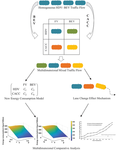
During the process of model construction, this study made the following assumptions:

1. All vehicles without lane-changing are running on the lane centerline, and the starting point of lane-changing vehicles is the lane centerline.

2. Lane-changing vehicles only change lanes to the right and leave lanes.

3. No vehicles enter the lane.

4. The velocity-energy consumption characteristics of the connected and manual vehicles are the same.

Multi-dimensional mixed traffic flow energy consumption model

To explore the internal relationship between the BEV penetration rate, CACC penetration rate, and traffic flow emissions, a multi-dimensional road section traffic flow energy consumption model was established to quantitatively analyze the emissions change in the traffic flow operation state.

For a traditional FV, the energy consumption calculation formula based on the power ratio is shown in Equation 1(1) $F_{\mathrm{f}\mathrm{u}\mathrm{e}\mathrm{l}}=\gamma \cdot Round(V{)}^{0.42}$(1) (Song and Yu 2019), which can better calculate the vehicle fuel consumption under frequent velocity changes.

(1) $F_{\mathrm{f}\mathrm{u}\mathrm{e}\mathrm{l}}=\gamma \cdot Round(V{)}^{0.42}$(1)

where $F_{\mathrm{f}\mathrm{u}\mathrm{e}\mathrm{l}}$is the instantaneous fuel consumption of FV, in g/s; $\gamma$ is the vehicle coefficient, which is related to the vehicle weight, load, traction power, and comprehensive calculation value 1.71; $V$ is the vehicle power ratio, which is related to vehicle velocity $v_n(t)$ and acceleration ${\dot{v}}_n(t)$, which is calculated using Equation 2; and $Round(V)$ is the nearest integer value of the power ratio.

(2) $V=v_n(t)(1.1{\dot{v}}_n(t)+0.132)+(3.02\times {10}^{-4})v_n^3(t)$(2)

Considering that there is a certain proportion of BEVs in the mixed traffic flow, Equation 3 is used to calculate the energy consumption of the BEV (Bekta and Laporte 2011).

(3) $F_{\mathrm{e}\mathrm{l}\mathrm{e}}={\dot{v}}_n(t)(w_1+w_2)+0.5C_{d}A{\rho }_{air}{v}_n^2(t)$(3)

where $F_{\mathrm{e}\mathrm{l}\mathrm{e}}$ is the unit energy consumption of the BEV, in J/m; $w_1$ and $w_2$ are the weight and load of the vehicle, respectively; $(w_1+w_2)$ is 1500 kg; $C_d$ is the traction coefficient, taken as 0.7; $A$ is the windward area of the vehicle, taken as 0.378 m²; and ${\rho }_{air}$ is the air density, generally 1.2041 kg/m³.

Owing to the different measurement units and different energies released by FVs and BEVs, to perform consistent statistics on the energy consumption of FV-BEV mixed traffic flow, gasoline and electric power were converted into standard coal energy consumption equivalent values in proportion according to the General Principles for Calculation of Comprehensive Energy Consumption (GB/T2589–2020), as shown in Equations 4(4) $C_{\mathrm{f}\mathrm{u}\mathrm{e}\mathrm{l}}=\frac{\sum _t{F}_{\mathrm{f}\mathrm{u}\mathrm{e}\mathrm{l}}{\kappa }_{\mathrm{f}\mathrm{u}\mathrm{e}\mathrm{l}}}{10}$(4) and 5(5) $C_{\mathrm{e}\mathrm{l}\mathrm{e}}=\frac{\sum _l{F}_{\mathrm{e}\mathrm{l}\mathrm{e}}{\kappa }_{\mathrm{e}\mathrm{l}\mathrm{e}}}{10}$(5) .

(4) $C_{\mathrm{f}\mathrm{u}\mathrm{e}\mathrm{l}}=\frac{\sum _t{F}_{\mathrm{f}\mathrm{u}\mathrm{e}\mathrm{l}}{\kappa }_{\mathrm{f}\mathrm{u}\mathrm{e}\mathrm{l}}}{10}$(4)

where $C_{\mathrm{f}\mathrm{u}\mathrm{e}\mathrm{l}}$ is the energy consumption per hundred kilometers of FV traffic flow in the road section, ${\kappa }_{\mathrm{f}\mathrm{u}\mathrm{e}\mathrm{l}}$ is the coal conversion coefficient of gasoline (1.4714 kgce/kg), and $t$ is the time of statistics.

(5) $C_{\mathrm{e}\mathrm{l}\mathrm{e}}=\frac{\sum _l{F}_{\mathrm{e}\mathrm{l}\mathrm{e}}{\kappa }_{\mathrm{e}\mathrm{l}\mathrm{e}}}{10}$(5)

where $C_{\mathrm{e}\mathrm{l}\mathrm{e}}$ is the energy consumption per hundred kilometers of BEV traffic flow in the road section, ${\kappa }_{\mathrm{e}\mathrm{l}\mathrm{e}}$ is the electricity coal conversion coefficient (0.03412 kgce/MJ), and $l$ is length of statistical section.

In the homogeneous HDV traffic flow, the energy consumption curves of $C_{\mathrm{f}\mathrm{u}\mathrm{e}\mathrm{l}}$ and $C_{\mathrm{e}\mathrm{l}\mathrm{e}}$ are shown in Figure 2.

Figure 2. Emission curves of fuel vehicle and electric vehicle.

The marked point in Figure 2 is the minimum energy consumption point, which is also known as the economic velocity point. For FVs, when the vehicle velocity was 14.5 m/s, the energy consumption intensity reached the lowest level, which was 3.53 kgce/100 km. The inflection point of the BEV emissions curve is shifted to the left compared with FV, and the energy consumption intensity was only 1.9 kgce/100 km at 9.6 m/s. Before this point, the vehicle primarily works against the rolling resistance, and the energy consumption intensity gradually decreases with increasing velocity. After this point, the increase in velocity causes the air resistance to increase exponentially. Vehicles need to consume more energy when driving at a high velocity. The model energy consumption curve is consistent with relevant research (Graba et al. 2021).

When considering the CACC penetration rate, the HDV-CACC mixed traffic flow is different from the FV-BEV mixed traffic flow. HDV and CACC vehicles have no essential differences in energy and power. However, CACC has advantages such as intelligent networking and predictable controlling of the velocity. Therefore, HDV and CACC vehicles exhibit differences in velocity and acceleration when disturbances occur. The HDV constraint relationship in traffic flow is given by the classic intelligent driver model (IDM) equation (Treiber, Hennecke, and Helbing 2000):

(6) ${\dot{v}}_n(t)=a\left[1-{\left(\frac{v_n(t)}{v_f}\right)}^4-{\left(\frac{s_0+v_n(t)T_s+\frac{v_n(t)\mathrm{\Delta }v}{2\sqrt{ab}}}{h_n(t)-l}\right)}^2\right]$(6)

Where ${\dot{v}}_n(t)$ is the acceleration of vehicle $n$ at time $t$, $a$ is the maximum acceleration, $v_f$ is the free flow velocity, $v_n(t)$ is the velocity of vehicle $n$ at time $t$, $h_n(t)$ is the space headway of vehicle $n$ at time $t$, $l$ is the vehicle length, $s_0$ is the minimum parking spacing, $T_s$ is the safe time headway, $\mathrm{\Delta }v$ is the velocity difference, and $b$ is the comfortable deceleration. The HDV velocity and acceleration were extracted as $v_{\mathrm{H}}$ and ${\dot{v}}_{\mathrm{H}}$, respectively, by simulation.

During CACC car-following behavior, the feedback information of the front vehicle is added, and the feedback coefficient is introduced to derive the vehicle constraint relationship of HDV-CACC mixed traffic flow.

(7) ${\dot{v}}_n(t)=a\left[1-{\left(\frac{v_n(t)}{v_f}\right)}^4-{\left(\frac{s_0+v_n(t)T+\frac{v_n(t)\mathrm{\Delta }v}{2\sqrt{ab}}}{h_n(t)-l}\right)}^2\right]+r{\dot{v}}_{n-1}(t)$(7)

where $r$ is the front vehicle feedback coefficient; when $r=0$, it degenerates into the HDV car-following equation; and ${\dot{v}}_{n-1}(t)$ is the acceleration of the front vehicle at time $t$.

The velocity and acceleration of CACC vehicles were extracted as $v_{\mathrm{C}}$ and ${\dot{v}}_{\mathrm{C}}$, respectively.

In summary, the energy consumption for various scenarios of FV-BEV and HDV-CACC multi-dimensional mixed traffic flow is calculated as

(8) $\left(\begin{array}{ccc}\hspace{0.17em}& \mathrm{F}\mathrm{V}& \mathrm{B}\mathrm{E}\mathrm{V}\\ \mathrm{H}\mathrm{D}\mathrm{V}& C_1& C_3\\ \mathrm{C}\mathrm{A}\mathrm{C}\mathrm{C}& C_2& C_4\end{array}\right)=\left(\begin{array}{cc}0.1\sum _t\gamma \cdot Round{\left[\begin{array}{c}{v}_{\mathrm{H}}(1.1{\dot{v}}_{\mathrm{H}}+0.132)\\ +(3.02\times {10}^{-4})v_{\mathrm{H}}^3\end{array}\right]}^{0.42}{\kappa }_{\mathrm{f}\mathrm{u}\mathrm{e}\mathrm{l}}& 0.1\sum _l{\dot{v}}_{\mathrm{H}}(w_1+w_2)+0.5C_{d}A{\rho }_{air}{v}_{\mathrm{H}}^2{\kappa }_{\mathrm{e}\mathrm{l}\mathrm{e}}\\ 0.1\sum _t\gamma \cdot Round{\left[\begin{array}{c}{v}_{\mathrm{C}}(1.1{\dot{v}}_{\mathrm{C}}+0.132)\\ +(3.02\times {10}^{-4})v_{\mathrm{C}}^3\end{array}\right]}^{0.42}{\kappa }_{\mathrm{f}\mathrm{u}\mathrm{e}\mathrm{l}}& 0.1\sum _l{\dot{v}}_{\mathrm{C}}(w_1+w_2)+0.5C_{d}A{\rho }_{air}{v}_{\mathrm{C}}^2{\kappa }_{\mathrm{e}\mathrm{l}\mathrm{e}}\end{array}\right)$(8)

If the BEV penetration rate is $m$ and the CACC penetration rate is $p$ in the mixed traffic flow, the multi-dimensional mixed traffic flow energy consumption model is given by Equation 9(9) $C=\sum _d\left\{mn\left[(1-p)C_1+p{C}_2\right]+(1-m)n\left[(1-p)C_3+p{C}_4\right]\right\}$(9) :

(9) $C=\sum _d\left\{mn\left[(1-p)C_1+p{C}_2\right]+(1-m)n\left[(1-p)C_3+p{C}_4\right]\right\}$(9)

where $C$ is the intensity of the traffic flow energy consumption of the road section, in kgce/hundred kilometers; $n$ is the total number of vehicles; $d$ is the number of road lanes, and $C_1$, $C_2$, $C_3$, and $C_4$ are the four matrix elements in Equation 8(8) $\left(\begin{array}{ccc}\hspace{0.17em}& \mathrm{F}\mathrm{V}& \mathrm{B}\mathrm{E}\mathrm{V}\\ \mathrm{H}\mathrm{D}\mathrm{V}& C_1& C_3\\ \mathrm{C}\mathrm{A}\mathrm{C}\mathrm{C}& C_2& C_4\end{array}\right)=\left(\begin{array}{cc}0.1\sum _t\gamma \cdot Round{\left[\begin{array}{c}{v}_{\mathrm{H}}(1.1{\dot{v}}_{\mathrm{H}}+0.132)\\ +(3.02\times {10}^{-4})v_{\mathrm{H}}^3\end{array}\right]}^{0.42}{\kappa }_{\mathrm{f}\mathrm{u}\mathrm{e}\mathrm{l}}& 0.1\sum _l{\dot{v}}_{\mathrm{H}}(w_1+w_2)+0.5C_{d}A{\rho }_{air}{v}_{\mathrm{H}}^2{\kappa }_{\mathrm{e}\mathrm{l}\mathrm{e}}\\ 0.1\sum _t\gamma \cdot Round{\left[\begin{array}{c}{v}_{\mathrm{C}}(1.1{\dot{v}}_{\mathrm{C}}+0.132)\\ +(3.02\times {10}^{-4})v_{\mathrm{C}}^3\end{array}\right]}^{0.42}{\kappa }_{\mathrm{f}\mathrm{u}\mathrm{e}\mathrm{l}}& 0.1\sum _l{\dot{v}}_{\mathrm{C}}(w_1+w_2)+0.5C_{d}A{\rho }_{air}{v}_{\mathrm{C}}^2{\kappa }_{\mathrm{e}\mathrm{l}\mathrm{e}}\end{array}\right)$(8) , respectively. Equation 9(9) $C=\sum _d\left\{mn\left[(1-p)C_1+p{C}_2\right]+(1-m)n\left[(1-p)C_3+p{C}_4\right]\right\}$(9) can be used to calculate the traffic flow energy consumption based on the statistics of the velocity, acceleration, and other data. As shown in Figure 2, the economic velocity of traffic flow changes when the vehicle penetration rate of FV or CACC is altered, and the energy-consuming traffic flow velocity can be reversely calculated in the same way, which translates into a traffic flow velocity calculation model under the energy-consuming minimum goal.

Impact mechanism of lane-changing on energy consumption of mixed traffic flow

To calculate the traffic flow energy consumption of the actual traffic flow operation state, the microscopic traffic flow theory is used to study the influencing mechanism of vehicle lane changing on car-following behavior. As shown in Figure 3, ${\theta }_n$ is the angle between the centerline of the vehicle and the horizontal tangent line of the driving centerline, and $b_n$ is the offset distance between the centerline of the vehicle and the horizontal tangent line of the driving centerline.

Figure 3. Lane-changing behavior of the preceding vehicle.

The greater the value of ${\theta }_n$, the more remarkable the intention of the lane change, which forces the following traffic flow to slow down locally. To fully study the velocity change of the following car following the traffic flow of lane-changing vehicles, considering the lateral influence of vehicles, an increase in the lateral distance will promote the acceleration of vehicles. The velocity influence of the above two factors is the main reason for lane-changing behavior affecting traffic energy consumption. The lateral influence term and vehicle turning factor were introduced into the classic IDM, and the improved formula is shown in Equation 10(10) ${\dot{v}}_n(t)=a\left[1-{\left(\frac{v_n(t)}{v_f}\right)}^4-{\left(\frac{s_0+v_n(t)T+\frac{v_n(t)\mathrm{\Delta }v}{2\sqrt{ab}}}{h_n(t)-l}\right)}^2\right]+r{\dot{v}}_{n-1}(t)+\alpha Z(v_n(t))-\beta \frac{d}{dt}{\theta }_n(t)$(10) .

(10) ${\dot{v}}_n(t)=a\left[1-{\left(\frac{v_n(t)}{v_f}\right)}^4-{\left(\frac{s_0+v_n(t)T+\frac{v_n(t)\mathrm{\Delta }v}{2\sqrt{ab}}}{h_n(t)-l}\right)}^2\right]+r{\dot{v}}_{n-1}(t)+\alpha Z(v_n(t))-\beta \frac{d}{dt}{\theta }_n(t)$(10)

where $Z(v_n(t))$ is the lateral distance function, which is related to its own velocity, increases monotonically, and is a positive feedback; $\alpha$ is the lateral distance utility parameter; ${\theta }_n(t)$ is the vehicle steering angle function, which is positively related to ${\theta }_n$, and is a negative feedback; $\beta$ is the vehicle steering angle utility parameter; $T$ is the corrected headway and $T=T_s+\mathrm{\Delta }T$, where $\mathrm{\Delta }T$ is the corrected headway value.

$Z(v_n(t))$ was derived from literature 25 (Pham 2019), as shown in Equation 11:

(11) $Z(v_n(t))=\frac{\left(0.058v_n(t)+1.4728\right)-\mathrm{\Delta }{y}_n}{2}$(11)

where $\mathrm{\Delta }{y}_n$ is the lateral distance between the current vehicle and the lateral vehicle. Based on this assumption, the value in the model is the lane width.

The vehicle steering angle is shown in Figure 4. According to the mathematical geometric relationship, the Equation of ${\theta }_n(t)$ is:

Figure 4. Stability analysis diagram（$0.2\le r\le 0.5$. (a) $r=0.2$ (b) $r=0.3$ (c) $r=0.4$ (d) $r=0.5$.

(12) ${\theta }_n(t)=\frac{b_n}{h_n(t)-l}$(12)

Furthermore, the vehicle steering angle is affected by the disturbance $y_n(t)$ of the space headway, and Equation 12(12) ${\theta }_n(t)=\frac{b_n}{h_n(t)-l}$(12) can be expressed as:

(13) ${\theta }_n(t)=\frac{b_n}{h_n(t)+y_n(t)-l}=\frac{b_n}{h_n(t)-l}-\frac{b_n}{{\left(h_n(t)-l\right)}^2}{y}_n(t)$(13)

The time derivative can be used to obtain the rate of change of the vehicle angle with time under a spacing disturbance.

(14) $\frac{\mathrm{d}}{\mathrm{d}t}{\theta }_n(t)=-\frac{b_n}{{\left(h_n(t)-l\right)}^2}y{ }_n^{\prime }(t)=-\frac{b_n}{{\left(h_n(t)-l\right)}^2}h{ }_n^{\prime }(t)$(14)

where $y{ }_n^{\prime }(t)$ is the time derivative of $y_n(t)$, and $h{ }_n^{\prime }(t)$ is the time derivative of $h_n(t)$.

Because the interval $0.2\le r\le 0.5$ is relatively general (Qin et al. 2021) , to determine the value of the front vehicle feedback coefficient $r$, we further analyzed the sensitivity impact of stability on the front vehicle’s lane-changing behavior, as shown in Figure 4. When $r=0.4$ or $r=0.5$, lane-changing behavior has little impact on the stability of traffic flow. Even if the centerline of the vehicle deviates from the maximum, the unstable velocity range is only 0–0.65 m/s and 0–0.27 m/s, respectively. When $r=0.2$, the unstable velocity range increases to 1.25 m/s. When there is no lane-changing behavior, the stability of the system remains fragile. In summary, the feedback coefficient of CACC vehicles was used in the simulation of the traffic flow energy consumption model. The Nlinfit and Lsqcurvefit functions of MATLAB were used to fit the values of $\alpha$ and $\beta$, and the lateral distance utility parameter $\alpha =0.055$ and lateral offset utility parameter $\beta =8.5$ were obtained.

Simulation analysis of traffic flow energy consumption impact

Experimental design

As a powerful mathematical software, MATLAB integrates algorithm design, numerical analysis, modeling and simulation of dynamic systems. A MATLAB simulation experiment was used to compare and analyze the impact of the BEV penetration rate and CACC penetration rate on the energy consumption of car-following traffic flow, and the impact of lane-changing behavior on the energy consumption of multi-dimensional mixed traffic flow. The specifications of the computer used for the simulations are as follows: Operating System Windows 10, CPU i7-7700HQ with four logical cores, RAM DDR4 2133 MHz 8 G, Graphics NVIDIA GeForce GTX 1060 with 6GB GPU memory.

Macro configuration of simulated traffic flow

The vehicle status update rule is obtained via discretization of the constraint equation between vehicles, and its difference equation is

(15) $\left\{\begin{array}{c}{v}_n(t+\mathrm{\Delta }t)=v_n(t)+\mathrm{\Delta }t\cdot {\dot{v}}_n(t)\\ x_n(t+\mathrm{\Delta }t)=x_n(t)+\frac{v_n(t+\mathrm{\Delta }t)+v_n(t)}{2}\end{array}\right.$(15)

where $\mathrm{\Delta }t$ is the difference step size.

Figure 5 shows a basic diagram of the macro traffic flow based on the IDM. The left side increased to the free-flow area and each vehicle moved at the expected velocity. The average density was 12 veh/km. The right side decreased to the non-free-flow area. The vehicle velocity was limited and the average density was 65 veh/km. Table 1 shows the expected headway of dual drivers; the expected time headway of aggressive drivers was 1.2 s, and the expected time headway of conservative drivers was 2 s.

Figure 5. Basic diagram of IDM.

Table 1. Parameter calibration table.

Driver’s personality	Expected time headway
Aggressive	1.2 s
Conservative	2 s

In the simulation experiment, all are free-flow situations. $n$ vehicles are continuously dropped on the designated lane with a width of 3.75 meters. The arrival of vehicles follows the Poisson distribution. The expected density of the free-flow section is 12 veh/km. The ratio of aggressive to conservative drivers was set to 1:1 to control the density variance of the section. The CACC penetration rate $p$ and EV penetration rate $m$ was set to adjust the proportion of vehicle components in multi-dimensional mixed traffic flow.

The mixed flow runs at equilibrium velocity $v_{\mathrm{e}}$ at the initial moment, and then the disturbance caused by the leader vehicle decelerating or changing lanes breaks the balance state, and the disturbance propagates in pairs in the flow. The maximum simulation time was 3000 s, the simulation step was 0.1 s, and the initial velocity was 10 m/s. The parameters were selected according to Table 2. The values of $a$, $b$, $l$, and $s_0$ in the table refer to literature 27 (Shladover, Su, and Lu 2012).

Table 2. Parameter calibration table.

Parameter name	Notation	Value (unit)
Maximum acceleration	$a$	1（m/s^2）
Maximum deceleration	$b$	2 or 2.8（m/s^2）
Free flow velocity	$v_f$	22.2（m/s）
Vehicle length	$l$	5（m）
Minimum stopping distance	$s_0$	2（m）
Vehicle offset distance	$b_n$	0–1.5（m）
Correction time headway	$T$	1.86
Front vehicle feedback coefficient	$r$	0.3
Lateral distance utility parameter	$\alpha$	0.055
Lateral offset utility parameter	$\beta$	8.5
Number of lanes	$d$	1

Determination of effective impact section of lane change

To specifically analyze the impact of vehicle lane changing on energy consumption, it is necessary to compare the energy consumption within the effective disturbance impact length. The velocity difference between the front and rear vehicles during the disturbance process of lane changing is $\mathrm{\Delta }{v}_{ij}$, of which the maximum velocity deviation is $\mathrm{\Delta }{v}_{max}$. During the process of decreasing the disturbance, the effective disturbance index was calculated using Equation 16. The confidence level was 95%, and at $\delta \le \mathrm{\%}95$, it is the effective range of disturbance. The velocity impact when the disturbance was transmitted to a vehicle was less than 5%, and the subsequent traffic flow was no longer included in the statistical range.

(16) $\delta =\frac{\mathrm{\Delta }{v}_{max}-\mathrm{\Delta }{v}_{ij}}{\mathrm{\Delta }{v}_{max}}\times 100\mathrm{\%}$(16)

Test scenario design

To obtain reasonable test result data, five scenarios were set in this simulation.

Scenario 1: Randomly configure any traffic component proportion to simulate traffic flow. When the first vehicle changes lanes at a random time, the affected road sections are determined according to the method in 4.1.2, and an average of 10 simulation test structures is taken as the effective affected road sections for data statistics.

Scenario 2: Simulate the traffic situation when the BEV penetration rate changes from $p=0$ to $p=1$. Assume that all vehicles are driving in the centerline of the lane, all vehicles do not change lanes, and the CACC penetration rate is $p=0$. Calculate the cumulative energy consumption in the effective impact section and extract the relationship between the energy consumption and BEV penetration rate at each simulation velocity.

Scenario 3: Based on Scenario 2, simulate the traffic driving situation when the CACC penetration rate from $p=0$ to $p=1$; the BEV penetration rate is $m=0$; calculate the energy consumption of mixed traffic flow in the effective impact section, and analyze the impact of the CACC penetration rate on energy consumption.

Scenario 4: Simulation of 121 groups of traffic components composed of the BEV penetration rate and CACC penetration rate. The energy consumption of mixed traffic flow is counted in the effective impact section.

Scenario 5: Based on Scenario 4, the first vehicle changes lanes, and then count the energy consumption of mixed traffic flow under the proportion of 121 groups of traffic components in the effective impact section.

Simulation results

Impact analysis of EV penetration rate and CACC penetration rate

As shown in Figure 6, the cumulative energy consumption per hundred kilometers of traffic flow with the BEV penetration rate from $m=0$ to $m=1$ is obtained under Scenario 2. In addition to being affected by velocity, the cumulative energy consumption of FV-BEV mixed traffic flow is negatively related to the BEV penetration rate. The lower the BEV penetration rate, the lower the cumulative energy consumption of the traffic flow. When the BEV penetration rate is $m=1$, the homogeneous BEV traffic flow runs at an economic velocity of 9.6 m/s of electric vehicles, reaching the global minimum energy consumption point, with an energy consumption intensity of 189.88 kgce/100 km.

Figure 6. Energy consumption of each BEV penetration rate.

The marked curve represents the economic velocity for each BEV penetration rate. The economic velocity varies with the BEV penetration rate. This curve represents the velocity – BEV penetration rate relationship based on the minimum energy consumption. The economic velocity of traffic flow gradually increases from 9.6 m/s to 14.5 m/s when $m=1$. The analytical results are consistent with the energy consumption curve.

To clarify the impact of CACC vehicles on energy consumption in an intelligent networking environment, based on the simulation results of homogeneous HDV traffic flow energy consumption when the penetration rate of CACC vehicles in Scenario 3 is 0, the reduction rate of CACC impact energy consumption under homogeneous BEV traffic flow was calculated, as shown in Figure 7, to explore the impact of the CACC penetration rate on the minimum energy consumption point of traffic flow.

Figure 7. Traffic flow energy consumption reduction rate.

As shown in Figure 7, with an increase in the CACC penetration rate $p$, the energy consumption of the traffic flow decreased. When $p<0.5$, the reduction rate of traffic flow energy consumption was less than 15%. When $p\ge 0.6$, the reduction rate of traffic flow energy consumption increased. After transformation into a homogeneous CACC traffic flow, the energy consumption reduction rate in Scenario 3 reached 37.63%.

Impact analysis of lane-changing

As shown in Figure 8, the influence of lane-changing behavior on the minimum energy consumption point of HDV-CACC traffic flow was further considered. Under the same penetration rate, the energy consumption reduction rate in Scenario 5 was always less than that in Scenario 4. When $p<0.2$, the energy consumption of Scenario 5 considering lane-changing increased compared with the baseline. However, with an increase in the CACC penetration rate, the gap between the two scenarios gradually decreased. In general, under the condition of an arbitrary penetration rate, the impact of lane-changing behavior was always negative. The occurrence of lane-changing behavior destroyed the stability of traffic flow, causing the traffic to turn into an unstable state of driving and stopping. Frequent changes in acceleration, deceleration, and velocity led to increased energy consumption. However, even when considering the phenomenon of lane-changing behavior, the CACC penetration rate was conducive to reducing the energy consumption of traffic flow.

Figure 8. Comparison figure of traffic flow energy consumption reduction rate.

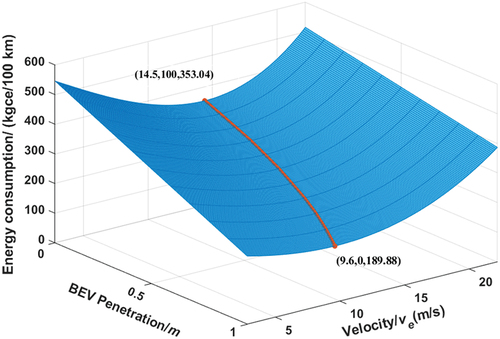
Figure 9 shows the energy consumption under the conditions of FV-BEV and HDV-CACC mixed traffic flows in Scenarios 4 and 5 when the BEV economic velocity is 9.6 m/s. Figure 9(a) shows the cumulative energy consumption without considering lane-changing behavior, and Figure 9(b) shows the cumulative energy consumption with consideration of lane-changing behavior.

Figure 9. Multi-dimensional mixed traffic flow energy consumption surface. (a) Without considering lane-changing. (b) Considering lane-changing.

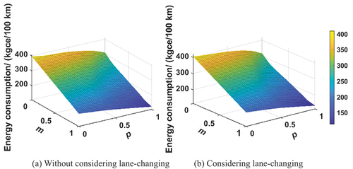
In Figure 9(a), the energy consumption of the traffic flow is related to the BEV penetration rate $m$ and CACC penetration rate $p$. Under the condition of homogeneous FV and HDV traffic flow, the energy consumption intensity reached 392 kgce/hundred kilometers. When BEV or CACC vehicles converged, energy consumption gradually decreased. When the traffic flow was transformed into homogeneous BEV and CACC, the energy consumption was only 128 kgce/hundred kilometers. Figure 9(b) fully considers lane-changing behavior, which is similar to Figure 8(a); however, the energy consumption curve is rising overall. The maximum energy consumption was higher than 400 kgce/100 km, and the minimum energy consumption intensity was 118.5 kgce/100 km. Lane-changing behavior increased the cumulative energy consumption of the traffic flow by 7.8% on average.

Conclusion

1. At any penetration rate, vehicle lane-changing behavior will increase the emissions of traffic flow, and the energy consumption of traffic flow with lane-changing behavior will increase by 7.8% on average compared with that of car-following traffic flow. At a certain BEV penetration rate, the influence of lane-changing behavior will gradually decrease with an increase in the CACC penetration rate. When the CACC penetration rate is $p=0.2$, the negative impact of lane-changing behavior is offset by the influx of CACC vehicle groups. At this time, the emissions of mixed traffic flow is equivalent to that of homogeneous HDV traffic flow. When $p=1$, lane-changing behavior only increases the traffic flow energy consumption by 4.99%, which is lower than the average level. In environments with low CACC penetration rates, frequent lane changes should be restricted. If a directional lane organization is adopted, emissions can be effectively reduced.

2. An increase in the BEV penetration rate can reduce the overall emissions of traffic flow. When driving at an economic velocity, the cumulative energy consumption of the homogeneous BEV traffic flow is only 58.3% that of the homogeneous FV traffic flow. During the gradual transformation of FV to BEV, there is a corresponding relationship between the traffic flow velocity at the minimum energy consumption point and the FV-BEV ratio. Based on the goal of achieving minimum emissions, the velocity of mixed traffic flow can be limited or induced according to the mixed FV-BEV ratio. This strategy can keep the air pollution caused by traffic emissions at the lowest level.

3. In this study, an energy consumption impact analysis method for mixed traffic flow is established based on the traffic flow car-following theory for multi-dimensional environments such as FV-BEVs and HDV-CACC. This model can adapt to mixed traffic flow with different penetration rates and acceleration feedback coefficients, and vehicle lane-changing behavior is considered, providing a decision-making basis for the traffic and environmental protection department to control the emissions of mixed traffic flow and protect air quality. It provides theoretical support for vehicle enterprises to optimize the development of electric vehicles and intelligent network-connected vehicles. However, in the energy consumption model in this study, only the BEV was considered. In the future, detailed modeling should be performed for hybrid, plug-in, and other new energy vehicles (such as those using hydrogen energy).

CRediT authorship contribution statement

Xinghua Hu: Conceptualization, Methodology, Software, Writing-original draft, Writing-review & editing, Data curation, Visualization, Supervision. Mintanyu Zheng: Conceptualization, Methodology, Software, Writing-original draft, Writing-review & editing. Jianpu Guo: Methodology, Formal analysis, Writing-original draft, Data curation, Supervision. Xinghui Chen: Software, Data curation, Writing-review & editing, Investigation. Gao Dai: Data curation, Investigation, Project Administration. Jiahao Zhao: Data curation, Visualization. Bing Long: Investigation, Formal analysis.

Abbreviations

Table

BEV	Battery electric vehicle
CACC	Cooperative adaptive cruise control
FV	Fuel vehicle
FV-BEV	Fuel vehicle-battery electric vehicle
HDV-CACC	Human-driven vehicle-cooperative adaptive cruise control

Disclosure statement

No potential conflict of interest was reported by the authors.

Data availability statement

Due to the nature of this research, participants of this study did not agree for their data to be shared publicly, so supporting data is not available.

Additional information

Funding

This research was supported in part by Sichuan Science and Technology Program under [Grant No. 2022YFG0132], and in part by the Chongqing Postgraduate Joint Training Base Project (Chongqing Jiaotong University-Chongqing YouLiang Science & Technology Co., Ltd Joint Training Base for Postgraduates in Transportation) under [Grant JDLHPYJD2019007].

Notes on contributors

Xinghua Hu

Xinghua Hu is a professor in the School of Traffic and Transportation at the Chongqing Jiaotong University. His research interest include on green transportation, intelligent transportation and transportation planning.

Mintanyu Zheng

Mintanyu Zheng is currently a postgraduate student in the School of Traffic and Transportation at the Chongqing Jiaotong University. His research focus is on the traffic flow energy consumption.

Jianpu Guo

Jianpu Guo is associate researcher in the Development of Science and Technology Statistics and Innovation, Chongqing Productivity Council.

Xinghui Chen

Xinghui Chen is currently a postgraduate student in the School of Traffic and Transportation at the Chongqing Jiaotong University.

Gao Dai

Gao Dai is professor level senior engineer in the Department of Technology R&D at the Chongqing YouLiang Science & Technology Co., Ltd.

Jiahao Zhao

Jiahao Zhao has a doctoral degree from the Beijing Jiaotong University. He is currently a senior lecturer in the School of Traffic and Transportation at the Chongqing Jiaotong University.

Bing Long

Bing Long is senior engineer in the Development of Traffic Engineering, Institute of Chongqing Transport Planning.

References

- Ahn, K., and H. A. Rakha. 2022. Developing a hydrogen fuel cell vehicle (HFCV) energy consumption model for transportation applications. Energies 15 (2):529. doi:10.3390/en15020529.
- Bekta, T., and G. Laporte. 2011. The pollution-routing problem. Transp. Res. Part B 45 (8):1232–50. doi:10.1016/j.trb.2011.02.004.
- Cattin, J., L. Leclercq, F. Pereyron, and N. E. Faouzi. 2019. Calibration of Gipps’ car-following model for trucks and the impacts on fuel consumption estimation. IET Intel. Transport Syst. 13 (2):367–75. doi:10.1049/iet-its.2018.5303.
- Devi, Y.U., and M.S. Rukmini. 2016. IoT in connected vehicles: Challenges and issues—a review. 2016 International Conference on Signal Processing, Communication, Power and Embedded System (SCOPES), 1864–67. IEEE.
- Ding, H., W. Li, N. Xu, and J. Zhang. 2022. An enhanced eco-driving strategy based on reinforcement learning for connected electric vehicles: Cooperative velocity and lane-changing control. J. Intell. Connected Veh. 5 (3):316–32. doi:10.1108/JICV-07-2022-0030.
- Editorial office of China Journal of Highway and Transport. 2016. Review on China’s traffic engineering research progress: 2016. China J. Highway Transp. 29 (6):1–161.
- Frey, H.C. 2018. Trends in onroad transportation energy and emissions. J. Air Waste Manag. Assoc. 68 (6):514–63. doi:10.1080/10962247.2018.1454357.
- Graba, M., J. Mamala, A. Bieniek, and Z. Sroka. 2021. Impact of the acceleration intensity of a passenger car in a road test on energy consumption. Energy 226:120429. doi:10.1016/j.energy.2021.120429.
- Haustein, S., A.F. Jensen, and E. Cherchi. 2021. Battery electric vehicle adoption in Denmark and Sweden: Recent changes, related factors and policy implications. Energy Policy 149:112096. doi:10.1016/j.enpol.2020.112096.
- Helbing, D. 2001. Traffic and related self-driven many-particle systems. Rev. Mod. Phys. 73 (4):1067. doi:10.1103/RevModPhys.73.1067.
- Hu, X., Y.M. Xu, J. Guo, T. Zhang, Y.H. Bi, W. Liu, and X. Zhou. 2022. A complete information interaction-based bus passenger flow control model for epidemic spread prevention. Sustainability 14 (13):8032. doi:10.3390/su14138032.
- Hu, X., and M. Zheng. 2021. Research progress and prospects of vehicle driving behavior prediction. World Electr. Veh. J. 12 (2):88. doi:10.3390/wevj12020088.
- Karelina, M.Y., P.I. Smirnov, and B.S. Subbotin. 2021. The influence of the characteristics of the traffic flow and the structure of vehicles on the energy consumption and ecological safety of passenger transportation: Case of Vologda, Russia. 2021 Intelligent Technologies and Electronic Devices in Vehicle and Road Transport Complex (TIRVED), Moscow, Russian Federation, 1–6. IEEE.
- Kaza, N. 2020. Urban form and transportation energy consumption. Energy Policy 136:111049. doi:10.1016/j.enpol.2019.111049.
- Kurien, C., A.K. Srivastava, and E. Molere. 2020. Indirect carbon emissions and energy consumption model for electric vehicles: Indian scenario. Integr. Environ. Assess. Manag. 16 (6):998–1007. doi:10.1002/ieam.4299.
- Lashgari, A., H. Hosseinzadeh, M. Khalilzadeh, B. Milani, A. Ahmadisharaf, and S. Rashidi. 2022. Transportation energy demand forecasting in Taiwan based on metaheuristic algorithms. Energy Sources, Part A 44 (2):2782–800. doi:10.1080/15567036.2022.2062072.
- Lin, B., and L. Shi. 2022. Do environmental quality and policy changes affect the evolution of consumers’ intentions to buy new energy vehicles. Appl. Energy 310:118582. doi:10.1016/j.apenergy.2022.118582.
- Liu, J.H., L. Feng, and Z.W. Li. 2021. Optimal road grade design based on stochastic speed trajectories for minimising transportation energy consumption. IET Intel. Transport Syst. 15 (11):1414–28. doi:10.1049/itr2.12111.
- Long, Y., Y. Yoshida, J. Meng, D. Guan, L. Yao, and H. Zhang. 2019. Unequal age-based household emission and its monthly variation embodied in energy consumption–a cases study of Tokyo, Japan. Appl. Energy 247:350–62. doi:10.1016/j.apenergy.2019.04.019.
- Luin, B., S. Petelin, and F. Al-Mansour. 2019. Microsimulation of electric vehicle energy consumption. Energy 174:24–32. doi:10.1016/j.energy.2019.02.034.
- Mekker, M. M., Y. J. Lin, M. K. I. Elbahnasawy, T. Shamseldin, H. Li, A. Habib, and D. Bullocck. 2018. Application of LiDAR and connected vehicle data to evaluate the impact of work zone geometry on freeway traffic operations. Transp. Res. Rec. 2672 (16):1–13. doi:10.1177/0361198118758050.
- Mohammad, A., and K.Ç. Merve. 2022. Prediction of transportation energy demand by novel hybrid meta-heuristic ANN. Energy 249:123735. doi:10.1016/j.energy.2022.123735.
- Montgomery, H. 2017. Preventing the progression of climate change: One drug or polypill? Biofuel. Res. J. 4 (1):536. doi:10.18331/BRJ2017.4.1.2.
- Nagel, K., and M. Schreckenberg. 1992. A cellular automaton model for freeway traffic. J. Phys. 2 (12):2221–29. doi:10.1051/jp1:1992277.
- Pham, Q.T. 2019. Investigation of avoidance assistance system for the driver of a personal transporter using personal space: A simulation based study. Int. J. Mech. Eng. Robot. Res. 8 (02):254–59. doi:10.18178/ijmerr.8.2.254-259.
- Qin, Y.Y., X.H. Hu, S. Q. Li, Z.Y. He, and M.T. Xu. 2021. Stability analysis of mixed traffic flow in connected and autonomous environment. J. Harbin Inst. Tech. 53 (3):152–57.
- Rahimi, M., D. Bortoluzzi, and F. Biral. 2022. Impacts of Vehicle Speed and Number of Heavy Vehicles on Emissions and Fuel Consumption in Sensitive Locations. CA: Transportation Research Record. 03611981221137586.
- Shladover, S.E., D. Su, and X.Y. Lu. 2012. Impacts of cooperative adaptive cruise control on freeway traffic flow. Transp. Res. Rec. 2324 (1):63–70. doi:10.3141/2324-08.
- Silgu, M.A., I.G. Erdağı, G. Göksu, and H.B. Celikoglu. 2021. Combined control of freeway traffic involving cooperative adaptive cruise controlled and human driven vehicles using feedback control through SUMO. IEEE Trans. Intell. Transp. Syst. 23 (8):11011–25. doi:10.1109/TITS.2021.3098640.
- Silgu, M.A., K. Muderrisoglu, A.H. Unsal, and H.B. Celikoglu. 2018. Approximation of emission for heavy duty trucks in city traffic. 2018 IEEE International Conference on Vehicular Electronics and Safety (ICVES), Madrid, Spain, 1–4. IEEE.
- Song, G.H., and L. Yu. 2019. Estimation of fuel efficiency of road traffic by characterization of vehicle-specific power and speed based on floating car data. Transp. Res. Rec. 2139 (1):11–20. doi:10.3141/2139-02.
- Tian, H.H., Y. Xue, S.J. Kang, and Y.J. Liang. 2009. Study on the energy consumption using the cellular automaton mixed traffic model. Acta Phys. Sin. 58 (7):4506–13. doi:10.7498/aps.58.4506.
- Treiber, M., A. Hennecke, and D. Helbing. 2000. Congested traffic states in empirical observations and microscopic simulations. Phys. Rev. 62 (2):1805–24. doi:10.1103/PhysRevE.62.1805.
- Watts, N., M. Amann, N. Arnell, S. Ayeb-Karlsson, K. Belesova, M. Boykoff, P. Byass, W. Cai, D. Campbell-Lendrum, S. Capstick and J. Chambers. 2019. The 2019 report of the lancet countdown on health and climate change: Ensuring that the health of a child born today is not defined by a changing climate. The Lancet 394 (10211):1836–78. doi:10.1016/S0140-6736(19)32596-6.
- Yang, C., and C. Huang. 2022. Quantitative mapping of the evolution of AI policy distribution, targets and focuses over three decades in China. Technol. Forecast. Soc. Change 174:121188. doi:10.1016/j.techfore.2021.121188.
- Yuan, T., F. Alasiri, and P.A. Ioannou. 2022. Selection of the speed command distance for improved performance of a rule-based VSL and lane change control. IEEE Trans. Intell. Transp. Syst. 23 (10):19348–57. doi:10.1109/TITS.2022.3157516.
- Zegeye, S.K., B. Schutter, J. Hellendoorn, E. Breunesseb, and A. Hegyic. 2013. Integrated macroscopic traffic flow, emission, and fuel consumption model for control purposes. Transp. Res. Part C 31:158–71. doi:10.1016/j.trc.2013.01.002.
- Zhang, Y. 2022. Analysis of China’s energy efficiency and influencing factors under carbon peaking and carbon neutrality goals. J. Clean. Prod. 370:133604. doi:10.1016/j.jclepro.2022.133604.
- Zhang, W., and W. Zhang. 2009. Boundary effects on energy dissipation in a cellular automaton model. Arxiv: Physicssoc-Ph. 0904.3727v2. https://doi.org/10.48550/arXiv.0904.3940
- Zhang, Y., Y. Zou, Y. Wang, L. Wu, and W. Han. 2022. Understanding the merging behavior patterns and evolutionary mechanism at freeway on-ramps. J. Intell. Transp. Syst. 26 (1):1–14. doi:10.1080/15472450.2022.2069501.
- Zhao, F., X. Liu, H. Zhang, Z. Liu, and W. Zhang. 2022. Automobile Industry under China’s carbon peaking and carbon neutrality goals: Challenges, opportunities, and coping strategies. J. Adv. Transp. 2022:5834707. doi:10.1155/2022/5834707.