Non-nulling protocols for fast, accurate, 3-D velocity measurements in stacks

ABSTRACT

The authors present protocols for making fast, accurate, 3D velocity measurements in the stacks of coal-fired power plants. The measurements are traceable to internationally-recognized standards; therefore, they provide a rigorous basis for measuring and/or regulating the emissions from stacks. The authors used novel, five-hole, hemispherical, differential-pressure probes optimized for non-nulling (no-probe rotation) measurements. The probes resist plugging from ash and water droplets. Integrating the differential pressures for only 5 seconds determined the axial velocity V_a with an expanded relative uncertainty U_r(V_a) ≤ 2% of the axial velocity at the probe’s location, the flow’s pitch (α) and yaw (β) angles with expanded uncertainties U(α) = U(β) = 1 °, and the static pressure p_s with U_r(p_s) = 0.1% of the static pressure. This accuracy was achieved 1) by calibrating each probe in a wind tunnel at 130, strategically-chosen values of (V_a, α, β) spanning the conditions found in the majority of stacks (|α| ≤ 20 °; |β| ≤ 40 °; 4.5 m/s ≤ V_a≤27 m/s), and 2) by using a long-forgotten definition of the pseudo-dynamic pressure that scales with the dynamic pressure. The resulting calibration functions span the probe-diameter Reynolds number range from 7,600 to 45,000.

Implications: The continuous emissions monitoring systems (CEMS) that measure the flue gas flow rate in coal-fired power plant smokestacks are calibrated (at least) annually by a velocity profiling method. The stack axial velocity profile is measured by traversing S-type pitot probes (or one of the other EPA-sanctioned pitot probes) across two orthogonal, diametric chords in the stack cross-section. The average area-weighted axial velocity calculated from the pitot traverse quantifies the accuracy of the CEMS flow monitor. Therefore, the flow measurement accuracy of coal-fired power plants greenhouse gas (GHG) emissions depends on the accuracy of pitot probe velocity measurements. Coal-fired power plants overwhelmingly calibrate CEMS flow monitors using S-type pitot probes. Almost always, stack testers measure the velocity without rotating or nulling the probe (i.e., the non-nulling method). These 1D non-nulling velocity measurements take significantly less time than the corresponding 2D nulling measurements (or 3D nulling measurements for other probe types). However, the accuracy of the 1D non-nulling velocity measurements made using S-type probes depends on the pitch and yaw angles of the flow. Measured axial velocities are accurate at pitch and yaw angles near zero, but the accuracy degrades at larger pitch and yaw angles.

The authors developed a 5-hole hemispherical pitot probe that accurately measures the velocity vector in coal-fired smokestacks without needing to rotate or null the probe. This non-nulling, 3D probe is designed with large diameter pressure ports to prevent water droplets (or particulates) from obstructing its pressure ports when applied in stack flow measurement applications. This manuscript presents a wind tunnel calibration procedure to determine the non-nulling calibration curves for 1) dynamic pressure; 2) pitch angle; 3) yaw angle; and 4) static pressure. These calibration curves are used to determine axial velocities from 6 m/s to 27 m/s, yaw angles between ±40°, and pitch angles between ±20°. The uncertainties at the 95% confidence limit for axial velocity, yaw angle, and pitch angle are 2% (or less), 1°, and 1°, respectively. Therefore, in contrast to existing EPA-sanctioned probes, the non-nulling hemispherical probe provides fast, low uncertainty velocity measurements independent of the pitch and yaw angles of the stack flow.

Introduction

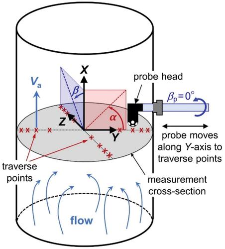
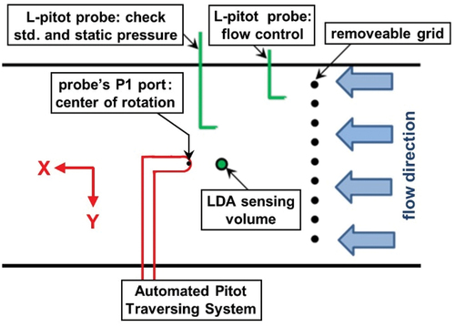
In 2020, anthropogenic carbon dioxide emissions totaled (34.8 ± 1.8)×10¹² kg (Friedlingstein et al. 2021). Coal-fired power plants produced 40% of these emissions. Thus, accurate, internationally accepted measurements of coal-fired plant emissions are essential for abating the CO₂ contributions to global climate change. In the United States, emissions from coal-fired power plants are determined by measuring the axial velocity V_a at prescribed locations in a cross-section of the plant’s exhaust stack. (Figure 1). The protocols for measuring V_a must be accepted by the U.S. Environmental Protection Agency (EPA). The most frequently used protocol deduces V_a from measurements of the pressure difference between the two holes of an S-probe oriented parallel to the stack axis (EPA 2017a, 2017c). This protocol can overpredict emissions by 10% or more when the flow in a stack has significant non-axial velocity components (Norfleet, Muzio, and Martz 1998). Here, the authors describe new protocols for measuring V_a that have much smaller expanded uncertainties¹ U_r(V_a) ≤ 2% and are traceable to internationally accepted standards. These uncertainties apply to stack flows with axial velocities 4.5 m/s ≤ V_a ≤ 27 m/s and with significant pitch (−20 ° ≤ α ≤ 20 °) and yaw (−40 ° ≤ β ≤ 40 °). (Figure 1 defines pitch and yaw). The authors believe that the new protocols are as robust and economical as the existing S-probe protocol, yet the non-nulling method outperforms existing methods by providing 2% accuracy or better for a wide range of yaw and pitch angles; therefore, they are attractive to the owners and regulators of power plants.

Figure 1. Schematic illustrates a non-nulling pitot probe traverse in a coal-fired power plant smokestack. A hemispherical probe measures the axial velocity (V_a) at traverse points located along the Y and Z axes. The flow’s pitch (α) and yaw (β) angles are defined relative to the direction of traverse paths and quantify the non-axial velocity components.

Methodolgy

Recently, the authors reported significant progress in generating fast, accurate, low-uncertainty protocols (Johnson et al. 2020). The authors used EPA-approved 5-hole spherical probes to measure V_a with the relative expanded uncertainty U_r(V_a) = 2% for the range 4.5 m/s ≤ V_a≤ 27 m/s, thereby avoiding the over-prediction problem inherent with S-probe measurements (Norfleet, Muzio, and Martz 1998). These demonstration measurements were conducted in a fast (therefore economical), non-nulling mode. (In the nulling mode the spherical probe is rotated about its axis until the pressure difference between designated holes is zero. This time-consuming process is repeated at each measurement location.) The demonstrated speed and accuracy of these non-nulling measurements were encouraging; however, these measurements revealed two problems that the authors address in this manuscript. (1) The pressure ports of the spherical probe frequently became plugged by ash and/or by water droplets entrained in the exhaust gas. The diameter of the spherical probe’s ports was 1.5 mm, much smaller than the 12.7 mm diameter of the S-probe’s ports. (2) The authors calibrated each spherical probe at 3000 values of (V_a, α, β) in NIST’s wind tunnel. Such extensive calibrations are expensive and not generally available; therefore, they cannot be the basis of a widely used protocol.

Our solution to the plugging problem is the novel, 5-hole hemispherical probe described in Section 3, below. This patented non-nulling hemispherical probe features large 6.5 mm ports that minimize plugging problems when used with stack measurement applications (Shinder, Johnson, and Filla 2022).

Our solution to the calibration problem is described in Section 3, below. It combines 3 ideas: (1) including V_a, or equivalently, the probe-diameter Reynolds number as an independent calibration variable (in addition to α and β), (2) using an unusual, judiciously-chosen definition of the pseudo-dynamic pressure to scale the differential pressure measurements, and (3), a systematic strategy for minimizing the number of calibration set-points. The authors combined these ideas to achieve a cost-effective procedure for using hemispherical probes throughout the 3-parameter space (|α | ≤ 20 °; |β | ≤ 40 °; 4.5 m/s ≤ V_a≤ 27 m/s) with expanded relative uncertainties U_r(V_a) ≤ 2% at each point. However, to achieve this low uncertainty at yaw angles near |β | ≈ 40 °, the authors had to increase the span of the yaw calibrations from |β | ≤ 40 ° to |β | ≤ 45 °.

In addition to solving the plugging and calibration problems, this manuscript deals with several other problems that relate to the practical application of five-hole hemispherical probes for fast, accurate 3D velocity measurements in stacks. In Section 4, the authors consider 7 identically-designed probes manufactured using different processes and materials. The dimensions of each probe were measured with a coordinate measuring machine (CMM), and the variability between probes was the basis of the hemispherical probe’s specified dimensional tolerances in Figure 4. By implementing the wind tunnel measurement protocol documented in Section 5 and the uncertainty analysis in Section 6, the authors verified that all 7 probes could be calibrated to achieve the target expanded relative uncertainties U_r(Va) ≤ 2% at each point. The dominant uncertainty for the calibration curves resulted from the residuals of fitting 3 variable, 3rd degree polynomials to the wind tunnel data. Therefore, low uncertainty non-nulling calibrations in the field will not require laboratory grade pressure sensors or state-of-the anemometers to achieve U_r(Va) ≤ 2% at each point. The authors expect hemispherical probes manufactured in accordance with Figure 4 can be calibrated to the obtain the target uncertainty U_r(V_a) ≤ 2% by following the measurement protocol in Section 5.

A committee of the American Society of Mechanical Engineers is drafting a documentary standard to facilitate EPA’s adoption of a non-nulling, hemispherical probe protocol for stack flow measurements. This publication provides technical details of the research and methods that are the basis of the documentary standard.

Hemispherical probe design

After evaluating a variety of 3D printed probe shapes and port orientations in the NIST wind tunnel, the authors selected a custom designed 5-hole hemispherical probe for further evaluation in stack flows. The wind tunnel results indicated that the hemispherical probe could be calibrated with low uncertainty using fewer points (See Section 3.3). During stack tests, the non-nulling hemispherical probe provided fast, accurate V_a measurements without rotating (or “nulling”) the probe or having its pressure ports blocked by particulates in the flue gas (Johnson et al. 2019). Figure 2 shows the shape and dimensions of the hemispherical probe’s head. The probe’s head consists of a bullet-shaped probe tip attached to a probe support at a 90° angle. During calibration and field applications a long shaft connects to the probe support to move the head to the desired position in a wind tunnel or stack. At each traverse point, the pressure is measured at 5 ports on the hemispherical surface of the probe’s tip. The central port is denoted port #1 and the four peripheral ports are denoted #2, #3, #4, and #5. The adjacent, peripheral ports are spaced 90° apart in the YʹZʹ plane, and the angle between the Xʹ-axis and a line segment extending from the center of the hemisphere to the center of any peripheral pressure port is γ = 40.5 °.

Figure 2. Five-hole hemispherical probe head. During the probe’s calibration, it was attached to a 1 m long, 25.4 mm O.D. carbon fiber tube. The support tube enclosed narrower, pressure-transmitting tubes that connected the ports in the probe’s head with differential-pressure gauges located several meters away.

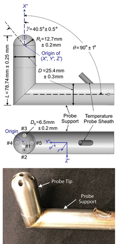
The radius of curvature of the hemispherical surface R_t = 12.7 mm is several times larger than similar five-hole probes used for atmospheric boundary layers measurements and turbomachinery applications (Hickman et al. 2021). The larger size is a key feature of our design because it facilitates larger diameter (D_b = 6.5 mm) pressure ports. Field tests in coal-fired stacks with wet scrubbers and dry scrubbers demonstrated that the larger hole size mitigates plugging of the pressure ports from water droplets or fly ash (Johnson et al. 2019). The forward-facing ports are 4.2 times larger than the ports on the EPA-approved spherical probe that is used for 3D velocity profiling in stacks (EPA 2017b). The larger holes on the hemispherical probe transition to smaller 1.65 mm diameter tubing inside the probe’s head. The probe’s head and support tube protect the tubing along the probe’s length. The tubing exiting the probe connects to differential pressure transducers located outside the wind tunnel or stack.

The probe’s tip is only L = 78.74 mm long; therefore, it fits through a standard stack flange (diameter 101.6 mm) without hitting the stack’s walls during the probe’s installation or removal. However, the 78.74 mm length is not sufficient to prevent flow interactions between the tip and the support. As a result of these interactions, the pressures at the ports differ from those that would exist without the support. These blockage effects increase at large negative pitch angles. Port #5, which is used to determine the pitch angle, is closest to the probe’s support and is most affected by blockage. Consequently, low uncertainty pitch angle determinations are limited by blockage effects. Here, the authors consider pitch angles in the range ± 20°, which exceeds the ± 12° range of pitch angles encountered in most stack flow measurements (Gentry 2019).

Calibration variables, pressure scaling, and set points

In this section, the authors describe: (1) V_a, or, equivalently, the probe-diameter Reynolds number (in addition to α and β) as an independent calibration variable, (2) selecting pressure-ratio scaling and variables to process the differential pressure measurements, and (3) minimizing the number of calibration set-points based on a systematic study of a “cost”-accuracy trade-off. The authors combined ideas to achieve a cost-effective procedure for calibrating hemispherical probes spanning the 3-parameter space (|α| ≤ 20 °; |β| ≤ 45 °; 4.5 m/s ≤ V_a≤ 27 m/s) with expanded relative uncertainties U_r(V_a) ≤ 2% at each calibration point.

Reynolds number is a calibration variable

In stack applications, the axial velocity V_a is the critical velocity component. In the notation of Figure 1, the magnitude of V_a is calculated by

(1) $V_{\mathrm{a}}=Vcos\beta cos\alpha .$(1)

where V is the magnitude of the velocity vector,

(2) $V=\sqrt{2p_{\mathrm{d}\mathrm{y}\mathrm{n}}/\rho }.$(2)

It equals the square-root of twice the dynamic pressure p_dyn divided by the gas density ρ. The pitch and yaw velocity components are defined by Vsinα and Vsinβ cosα, respectively.

In agreement with prior research, the authors found that the Reynolds number Re is useful for correlating the performance of five-hole probes (Dominy and Hodson 1992). The authors use the definition Re ≡ V_aD_t/ν, where ν is the kinematic viscosity and D_t = 2R_t is the diameter of the probe’s tip. For our probes, D_t = 25.4 mm and ν ≈15.1 × 10⁻⁶ m²/s for air nominally at ambient pressure and 20 °C; therefore, the velocity range 4.5 m/s ≤ V_a≤ 27 m/s corresponds to the range 7,600 ≤ Re ≤ 45,000. The significance of Re depends on the shape of the probe’s head (Azartash-Namin 2017), the value of the Re (Dudzinski and Krause 1969; Passmann et al. 2021; Wallen 1983), the pitch and yaw of the flow (Pisasale and Ahmed 2004; Treaster and Yocum 1979), and the intensity of the freestream turbulence (Dominy and Hodson 1992).

Pressure-ratio scaling and calibration variables

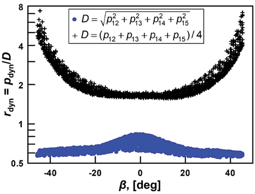
The authors used differential pressure transducers to measure the differences between the pressure at each port and the static pressure: p_is = p_i – p_s for i = 1 to 5. Then, the authors calculated the differences between the central port (port #1) and the 4 peripheral ports: p_1s = p_1s – p_is, for i = 2 to 5. Likewise, the yaw and pitch pressures were calculated by subtracting the corresponding port pressures, p₂₃ = p_2s – p_3s and p₄₅ = p_4s – p_5s, respectively. The authors define the pseudo-dynamic pressure (p_PSEUDO) for scaling pressure ratios:

(3) $p_{\mathrm{P}\mathrm{S}\mathrm{E}\mathrm{U}\mathrm{D}\mathrm{O}}=\sqrt{p_{12}^2+p_{13}^2+p_{14}^2+p_{15}^2},$(3)

where p₁₂ etc. are the pressure differences between each peripheral port and the central port. In 1970, Wright defined a similar “velocity factor” based on sums of squares (Wright 1970). The authors use capital letters in the subscript of p_pseudo to distinguish it from the widely used scaling p_pseudo = p₁ - p_avg introduced by Dudzinski where p_avg = (p₂+p₃+p₃+p₅)/4 (Dudzinski and Krause 1969). Our discussion concerning Figure 3 explains the advantages of p_pseudo over p_pseudo in the context of measuring stack flows that have high angularity.

Figure 3. Dynamic pressure ratio r_dyn versus yaw angle β for two scaling factors D. The plus symbols (+) use D = p_pseudo as defined by Dudzinski (Dudzinski and Krause 1969); the solid circles (

) use D = p_PSEUDO as proposed here in Equation (3)(3) $p_{\mathrm{P}\mathrm{S}\mathrm{E}\mathrm{U}\mathrm{D}\mathrm{O}}=\sqrt{p_{12}^2+p_{13}^2+p_{14}^2+p_{15}^2},$(3) . (Data from NIST’s wind tunnel spanning airspeeds from 4.5 m/s to 27 m/s and pitch angles α from −20 ° to 20 °).

The authors develop correlations using 5 pressure ratios. The dynamic pressure ratio is

(4a) $r_{\mathrm{d}\mathrm{y}\mathrm{n}}=p_{\mathrm{d}\mathrm{y}\mathrm{n}}/p_{\mathrm{P}\mathrm{S}\mathrm{E}\mathrm{U}\mathrm{D}\mathrm{O}},$(4a)

and the static pressure parameter is

(4b) $r_{1\mathrm{s}}=p_{1\mathrm{s}}/p_{\mathrm{P}\mathrm{S}\mathrm{E}\mathrm{U}\mathrm{D}\mathrm{O}}$(4b)

where p_1s = p₁ – p_s. The authors also define three pressure ratios given by

(4c) $\begin{array}{rl}& r_{12}=p_{12}/p_{\mathrm{P}\mathrm{S}\mathrm{E}\mathrm{U}\mathrm{D}\mathrm{O}},\\ & r_{23}=p_{23}/p_{\mathrm{P}\mathrm{S}\mathrm{E}\mathrm{U}\mathrm{D}\mathrm{O}},\\ & r_{45}=p_{45}/p_{\mathrm{P}\mathrm{S}\mathrm{E}\mathrm{U}\mathrm{D}\mathrm{O}}.\end{array}$(4c)

These pressure ratios are used as the independent variables of four non-nulling calibration curves: 1) the pitch angle, f_α(r₁₂, r₂₃, r₄₅); 2) the yaw angle, f_β (r₁₂, r₂₃, r₄₅); 3) the dynamic pressure ratio, f_rdyn (r₁₂, r₂₃, r₄₅); and 4) the static pressure parameter, f_r1s (r₁₂, r₂₃, r₄₅). The authors developed these calibration curves using linear regression to fit 3^rd degree polynomials to data acquired in NIST’s wind tunnel. See the appendix for explicit examples of the calibration curves’ fit coefficients.

Figure 3 demonstrates the advantage of the scaling parameter p_pseudo. The authors plotted the dynamic pressure ratio r_dyn as a function of β, as measured in NIST’s wind tunnel (Shinder et al. 2013; Shinder, Hall, and Moldover 2010). (See Section 5.) The 2000 data points span the ranges: |α| ≤ 20 °; |β| ≤ 45 °; and 4.5 m/s ≤ V_a≤ 27 m/s. The plotted solid circles () show r_dyn scaled by p_pseudo. These data are well-behaved for all values of β; therefore, it is easy to represent them by polynomial functions. In contrast, the plus symbols (+) in Figure 3 represent r_dyn scaled by p_pseudo, as specified by Dudzinski and widely used by others. For yaw angles −20 ° ≤ β ≤ 20 °, the ratio p_dyn/p_pseudo is smooth and varies by only 25%; therefore, it too can be represented by simple polynomial functions. However, at larger values of β, p_pseudo → 0 causing r_dyn to diverge (Pisasale and Ahmed 2002). In this region, Dudzinski’s p_pseudo is not a suitable scaling parameter.

An alternative method to circumvent the divergence of Dudzinski’ p_pseudo is to separate the measurement domain into 5 zones, one corresponding to each pressure port on the probe’s head (Gallington 1980; Paul, Upadhyay, and Jain 2011). When this is done, the port with the maximum pressure determines which zone is used to compute the velocity. As a result, the method of zones requires correlations for all 5 zones. Other researchers have avoided the divergence by using a scaling parameter that depends on wind tunnel parameters (e.g., p_dyn, p_t, and p_s). A drawback of this technique is that the pressure coefficients are not explicitly determined by port pressure measurements. Instead, the pressure coefficients must be determined iteratively using numerical methods (Pisasale and Ahmed 2002, 2004). Neither alternative provides the straightforward probe calibration and application the authors propose in this manuscript.

Selecting calibration set points

To meet the majority of stack-flow measurement needs, the authors calibrated probes in the 3-parameter space: |α| ≤ 20 °; |β| ≤ 45 °; 4.5 m/s ≤ V_a≤ 27 m/s. In this space, a complete calibration on a grid (for example: 5 ° steps in α and β at each of 11 values of V_a comprising n = 1881 calibration set points) would be too expensive for many applications. For this reason, non-nulling probes have often been calibrated at a single velocity in turbomachinery applications. Instead of a grid, the authors devised a novel, quasi-random scheme for selecting n calibration set points and the authors quantified the trade-off between reduced calibration uncertainty versus increasing n. The authors concluded that n = 130 judiciously-selected set points produces calibration curves f_α, f_β, and f_rdyn for the hemispherical probe that have random errors that, on average, are only 40% larger than the corresponding errors in an n = 2000 calibrations.

Figure 4 is one example of many experiments that the authors used to quantify the trade-off between reduced calibration uncertainty versus increasing the number of calibration points. To generate Figure 4, the authors calibrated hemispherical probe #7 in NIST’s wind tunnel at 2000 (V_a, α, β) set points at the turbulence intensity of 3%. The authors began the calibration at the lowest velocity 4.9 m/s and increased V_a logarithmically at successive set points reaching the maximum velocity 30 m/s at set point 2000. At each set point, α was randomly selected from the 41 values between −20 ° to 20 ° in 1° increments, and β was randomly selected from the 91 values between −45 ° to 45 ° in 1 ° increments. The authors fitted the data for f_rdyn, f_α, and f_β to polynomial functions of pressure ratios r₁₂, r₂₃, and r₄₅. These polynomials were used in Equation (5)(5) $f{\upsilon }_{\mathrm{n}}=\sqrt{f_{\mathrm{r}\mathrm{d}\mathrm{y}\mathrm{n}}}cos{f}_{\beta }cos{f}_{\alpha }.$(5) to determine the normal velocity calibration factor fυ_n for the n = 2000 data set,

Figure 4. Increasing uncertainty of calibrations as the number of calibration points is reduced from n = 2000. The empirical dashed curve has the equation u_n/u₂₀₀₀= 1 + 7000/n². for n = 130, the uncertainty is approximately 1.4×u₂₀₀₀ where u₂₀₀₀ = 0.0057 is the fractional standard deviation of the residuals of the normal velocity calibration factor (fυ_n) in Equation (5)(5) $f{\upsilon }_{\mathrm{n}}=\sqrt{f_{\mathrm{r}\mathrm{d}\mathrm{y}\mathrm{n}}}cos{f}_{\beta }cos{f}_{\alpha }.$(5) .

(5) $f{\upsilon }_{\mathrm{n}}=\sqrt{f_{\mathrm{r}\mathrm{d}\mathrm{y}\mathrm{n}}}cos{f}_{\beta }cos{f}_{\alpha }.$(5)

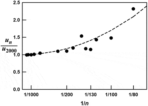
As a measure of the uncertainty of fitted values of fυ_n2000, the authors used u₂₀₀₀≡ StdDev{fυ_n2000/υ_n2000} = 0.0057. Here, the υ_n2000’s are the measured values of fυ_n2000, and the expression “StdDev{ … }” indicates the standard deviation calculated over the complete n = 2000 data set. The authors also computed fυ_n for 15 subsets of the n = 2000 set ranging in size from 60 ≤ n ≤ 2000. These mutually-independent, subsets were chosen by randomly removing velocity set-points from the n = 2000 set. For each subset the authors computed the ratio fυ_n/υ_n2000 where the υ₂₀₀₀ are the measured values of the scaled velocity calibration factor from the original, n = 2000 set, and the fυ_n’s are the calibration factors generated by fitting each of the 15 subsets to polynomial functions of the pressure ratios r₁₂, r₂₃, and r₄₅. The smooth, dashed curve in Figure 4 represents the fractional increase in uncertainty as n is reduced. The authors chose n = 130 as a compromise between accuracy and cost of probe calibrations. For n = 130, u₁₃₀/u₂₀₀₀ ≈1.4 and u₁₃₀ ≈0.8%.

The authors emphasize that u₁₃₀ ≈0.8% is the largest single contributor to the uncertainty of the measurement of V_a at a point in a stack. Knowing this, the authors chose to repeat the trade-off exercise after reducing the yaw range from |β | ≤ 45 ° to |β | ≤ 40 °. Because of the reduced range, u₂₀₀₀ decreased from 0.57% to 0.53%; u₁₃₀ decreased from 0.8% to 0.62%; and the equation of the dashed, trade-off curve in Figure 4 became: u_n/u₂₀₀₀ = 1 + 2800/n².

In the remainder of this paper, the authors use quasi-random, n = 130 calibrations generated by the following method. The first set point was the lowest velocity, V_a = 4.5 m/s. For this set point, a value of α was randomly selected from the nine 5 ° increments in the range from −20° to 20° and a value of β was selected from the ninety-one 1 ° increments of yaw angle between −45° to 45°. After completing measurements at these values (4.5 m/s, α, β), the authors increased the value of V_a by the factor 1.014 and randomly selected new values of α and β. This process was repeated until the maximum velocity 27 m/s was reached at the 130^th set point.

This calibration procedure exploits the fact that both α and β are weak functions of Reynolds number (Kjelgaard 1988), except at high yaw angles and low flow velocities where flow separation is prominent. An advantage of using small velocity increments is: the wind tunnel quickly stabilizes at successive set points. Because only 130 set points are needed, manual adjustment of the probe’s pitch and yaw at each set point is feasible.

Probe dimensions and interchangeablity

The authors purchased 7 custom hemispherical probes with dimensions specified in Figure 2. The authors measured the probes dimensions using a coordinate measuring machine (CMM). The probes were purchased from 3 different manufacturers, made from 2 different materials (plastic or stainless steel), and fabricated using 2 different processes (3D-printing or manually fabricated by machining and welding). Table 1 identifies each probe and lists its CMM measurements using the notation in Figure 2. The authors measured the angle θ between the probe tip and the probe support, the radius of curvature of the hemispherical surface R_t, the diameters D_b of the 5 pressure ports, the polar angles γ, and radial locations rʹ of the 5 ports. The table includes the averages and standard deviations of the port measurements of D_b, γ, and rʹ.

Table 1. Dimensional CMM measurements of 7 hemispherical probes all made in accordance with the probe design shown in Figure 2. (The uncertainty of the CMM measurements was 0.02 mm).

Probe No.	Manuf.	Material	Manuf. Process	θ [deg]	Rt [mm]	Db [mm]	center hole		4 peripheral holes
							γ [deg]	rʹ [mm]	γ [deg]	rʹ [mm]
1	A	stainless steel	manually fabricated	89.2	12.69 [0.045]^a	6.51 (0.016)^b	0.1	0.05	40.50 (0.14)	8.33 (0.038)
2	A	stainless steel	manually fabricated	91.3	12.76 [0.085]	6.511 (0.004)	0.1	0.14	40.88 (0.36)	8.34 (0.08)
3	B	stainless steel	3D Printed	90.6	12.54 [0.05]	6.40 (0.023)	0.2	0.05	40.85 (0.25)	8.21 (0.04)
4	B	plastic resin	3D Printed	89.9	12.66 [0.057]	6.46 (0.021)	0.2	0.1	40.95 (0.29)	8.29 (0.076)
5	B	plastic resin	3D Printed	90.0	12.66 [0.065]	6.45 (0.024)	0.3	0.07	40.95 (0.48)	8.27 (0.038)
6	C	plastic resin	3D Printed	90.0	12.66 [0.068]	6.41 (0.033)	0.1	0.11	40.28 (0.33)	8.17 (0.053)
7	C	stainless steel	3D Printed	88.7	12.64 [0.20]	6.41 (0.039)	0.3	0.07	40.58 (1.12)	8.2 (0.055)
			Average Stdev.	89.96 {0.85}c	12.686 {0.06}	6.51{0.016}	0.19	〈0.03〉d	40.5 {0.26}	8.26 {0.07}

^aSquare brackets “[]” denote the dimensional form error defined as the departure from measured radius of curvature.

^bRound brackets “()” denote the standard deviation of the related hole dimensions on the same probe (e.g., D_b of the 5 holes, γ or r ʹ of the peripheral ports).

^cCurly brackets “{}” denote the standard deviation of the same dimensions on different probes.

^dAngle brackets “〈〉” denote the average of radius of the center hole for all 7 probes as calculated using $r{ }^{\mathrm{\prime }}=\sqrt{Y{{ }^{\mathrm{\prime }}}_{\mathrm{a}\mathrm{v}\mathrm{g}}^2+Z{{ }^{\mathrm{\prime }}}_{\mathrm{a}\mathrm{v}\mathrm{g}}^2}$, where Yʹ_avg and Zʹ_avg are the respective averages of these coordinates for all 7 probes.

The authors deliberately varied the probes’ manufacturers, fabrication methods, and materials to determine how these variations impacted the probes’ non-nulling calibrations. If the calibrations were insensitive to these variations, the probes would be interchangeable; that is, calibration of a single hemispherical probe would accurately predict the performance of all the probes. However, our wind tunnel calibrations showed that each probe must be individually calibrated to ensure the expanded uncertainty of the axial velocity U_r(V_a) ≤ 2%. If the calibration of probe #3 is applied to the other probes, the average of 100 (V_a,p/V_a,3 − 1) = 4% where the average equally weights the full range of α, β and V_a,p and the index p indicates the probes other than #3. The authors were unable to use the dimensional measurements to correct probes’ calibration curves to a universal curve because: (1) the authors do not know the functional forms of the corrections, and (2) the expanded uncertainties of the CMM measurements (0.02 mm) are comparable to the errors in the hemispherical shape and to the standard deviations of the locations of the peripheral holes. Instead of developing corrections based on the dimensional measurements, the authors used the spans of the measurements to specify the tolerances listed in Figure 2. The authors are confident that probes satisfying these tolerances can be calibrated using the method proposed herein to achieve U_r(V_a) ≤ 2%.

Calibrating probes in NIST’s wind tunnel

Layout for calibrating probes in turbulence

The authors characterized the 7 hemispherical probes in the rectangular test section (1.5 m by 1.2 m) of NIST’s wind tunnel over velocities spanning 4.5 m/s to 27 m/s (Re = 7,600 to 45,000). The authors measured the air’s axial velocity V_LDA using NIST’s laser doppler anemometer (LDA) with a standard uncertainty of u_r(V_LDA) = 0.205% (Shinder et al. 2014). The top view of the test section depicted in Figure 5 shows the location of a hemispherical probe during calibrations in NIST’s wind tunnel. The LDA’s sensing volume was 12 cm upstream of the hemispherical probe’s port #1. To correct for blockage effects caused by the hemispherical probe and its support, the velocity measured by the LDA at x = 12 cm (V_LDA,12 cm) was multiplied by a blockage correction factor, C_blk,12 cm = 1.008 (Shinder et al. 2021). As indicated in Figure 5, the authors used the L-shaped pitot probe closest to the LDA’s sensing volume as a check standard to verify V_LDA and to measure the static pressure p_s. The output of another L-shaped pitot probe was used in a PID loop to control the wind speed in the test section. These pitot probes were located such that their blockage effects were negligible.

Figure 5. Schematic layout of instruments in the wind tunnel’s test section, as viewed from above, when calibrating a hemispherical pitot probe.

During the calibrations of each hemispherical probe, a turbulence-generating grid was located upstream of the probe under test (See Figure 5). The measurement of Tu and the corrections for the grid’s blockage are explained in (Shinder et al. 2021). In the absence of the grid, the turbulence intensity in NIST’s wind tunnel was so low (Tu ≈0.1%) that the laminar boundary layer on the surface of hemispherical probes became unstable leading to obvious hysteresis in the calibration curves at V_LDA≤ 5 m/s and |β | > 45 ° (Crowley et al. 2013). This hysteresis does not occur in turbulent stack flows nor does it occur when the grid-generated turbulence was Tu = 3%.

In the wind tunnel, the density of the air and the LDA’s velocity determine the dynamic pressure by

(6) $p_{dyn}=\rho V_{LDA}^2/2.$(6)

The authors determined the air’s density from measurements of the temperature, relative humidity, and static pressure p_s near the test section wall (not shown in Figure 5) using (Yeh and Hall 2007).

(7) $\rho =c_0/T\left[p_s-c_{1}RHexp\left(-c_2/T\right)\right].$(7)

Here, T is the Kelvin temperature, RH is the relative humidity in percent, and the coefficients c₀, c₁, and c₂ have the values: c₀ = 3.4848 × 10⁻³ K kg/J, c₁ = 6.65287 × 10⁸ Pa, and c₂ = 5315.56 K. The relative uncertainty of the density equation of state is u_r,EOS(ρ) = 0.1% (Jaeger and Davis 1984).

Differential pressure measurements

Static line pressure effects can affect the accuracy of the measured differential pressures p₁₂, p₁₃, p₁₄, and p₁₅. During probe calibration the port pressure p₁ varies at each of the probe’s pitch and yaw orientations. When a differential pressure transducer measures the difference between port pressures, p_1j for j = 2 to 5, the static line pressure changes in accordance with the variation in p₁. Our testing showed that some pressure transducers that are not equipped with line pressure compensation can yield readings outside their specifications when they are used at line pressures that differ from the line pressure used during calibration. The laboratory grade differential pressure transducers used in this work account for line pressure effects; however, the authors anticipate that the non-nulling protocol will be implemented using less expensive differential transducers commonly used in stack applications. Our suggested protocol for measuring p_1j minimizes uncertainty attributed to line pressure effects.

The authors used differential pressure transducers to measure the differences between the pressure at each port and the static pressure: p_is = p_i – p_s for i = 1 to 5. Then, the authors calculated the differences between the central port (port #1) and the 4 peripheral ports: p_1i = p_1s – p_is, for i = 2 to 5. Similar subtractions were used to calculate the yaw pressure p₂₃ = p_2s – p_3s and the pitch pressure p₄₅ = p_4s – p_5s. The authors re-zeroed the differential pressure transducers (as necessary) after each change in the velocity set point. The pseudo dynamic pressure is determined via Equation (3)(3) $p_{\mathrm{P}\mathrm{S}\mathrm{E}\mathrm{U}\mathrm{D}\mathrm{O}}=\sqrt{p_{12}^2+p_{13}^2+p_{14}^2+p_{15}^2},$(3) and the pressure ratios are calculated using (4a) through (4c).

Automated traversing system

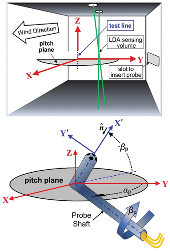
Figure 5 shows the probe’s orientation just after it was installed in the wind tunnel when its pitch and yaw angles are zero, α_p = 0 ° and β_p = 0 °, respectively. In this orientation, the probe’s head is parallel to the X-axis and located 12 cm downstream from the LDA’s sensing volume on the same streamline as the sensing volume. The authors set β_p = 0 ° by placing an inclinometer along the probe’s head in the X-direction and manually rotating the probe’s support about its axis until the inclinometer read zero. After zeroing β_p, the probe was securely fastened to the automated traverse system located just outside the wind tunnel (See Figure 5). The traverse system was used to orient the probe’s support shaft 90 ° to the wind tunnel wall’s so that α_p = 0 °.

During calibrations, NIST’s automated traversing system in Figure 6 orients the probe’s head to specified α_p and β_p while maintaining port #1 on the section of the Z-axis referred to as the test line indicated by dotted line () in Figure 6. As β_p spans ± 45 °, port #1 moves along the test line spanning a distance Z = ±5.6 cm. Throughout the calibration process, the dominant uncertainties of the probe’s yaw and pitch angles result from the pitch and yaw misalignment during the probe’s installation. The uncertainties resulting from the traverse system’s translational and rotational stages are only 0.01 mm and 0.015 °, respectively. The uncertainty of the yaw angle is u(β_p) = 0.25 °. The uncertainty of the pitch angle is slightly larger, u(α_p) = 0.35 ° because it includes the misalignment and an additional uncertainty resulting from aerodynamic drag on the probe. Section 5.6 discusses alignment and additional details regarding the traverse system are provided in reference (Shinder et al. 2021).

Figure 6. TOP: Wind tunnel’s coordinate system. The probe’s port #1 remains on the dashed test line during calibration. The coordinate system’s origin is located 12 cm downstream from the LDA’s sensing volume. BOTTOM: Coordinate system for orienting a hemispherical pitot probe. The probe’s pitch angle α_p is in the XY plane; it increases from zero as the probe’s shaft is rotated in the pitch plane from the Y-axis. The probe’s yaw angle β_p increases when the probe’s shaft is rotated about its axis. The axes X′ and Y′ are attached to the probe.

Data acquisition and probe calibration software

A custom software program controls the air speed and the probe’s pitch and yaw angle settings. The program also acquires the calibration data including the LDA velocity (V_LDA), the pressure measurements at each probe port (i.e., p_1s, p_2s, p_3s, p_4s, and p_5s), the probe’s pitch angle (α_p), and the probe’s yaw angle (β_p). Pressure-based instrument readings are acquired using a PCI-based multifunction DAQ board, while auxiliary LabVIEW programs are used to continuously monitor the LDA system, the temperature (T) and relative humidity (RH) of the wind tunnel air, and the static pressure (p_s). The program ensures that the flow is stable and within ± 0.2% of the velocity set point during data collection.

Data reduction and non-nulling calibration functions

When used in stacks, the probe is installed at β_p = 0° and α_p = 0° in the stack’s coordinate system (X, Y, Z) depicted in Figure 1. Conversely, during calibrations the authors orient the probe at specified values of α_p and β_p in the wind tunnel’s coordinate system (X, Y, Z) shown in Figure 6. The relationships between the flow’s relative yaw and pitch angles in the (X ʹ, Y ʹ, Z ʹ) coordinate system and the flow’s yaw and pitch angles in the (X, Y, Z) coordinate system are

(8a) $\beta { }^{\mathrm{\prime }}=\beta -{\beta }_p,$(8a)

and

(8b) $\alpha { }^{\mathrm{\prime }}=\alpha -{\alpha }_p,$(8b)

respectively.

The yaw and pitch calibration functions f_β and f_α are polynomials fitted to α ʹ and βʹ calibration data. Similarly, the dynamic pressure ratio and static pressure parameter functions, f_rdyn and f_r1s, are polynomials fitted to r_dyn in Equation (4a)(4a) $r_{\mathrm{d}\mathrm{y}\mathrm{n}}=p_{\mathrm{d}\mathrm{y}\mathrm{n}}/p_{\mathrm{P}\mathrm{S}\mathrm{E}\mathrm{U}\mathrm{D}\mathrm{O}},$(4a) and r_1s in Equation (4b)(4b) $r_{1\mathrm{s}}=p_{1\mathrm{s}}/p_{\mathrm{P}\mathrm{S}\mathrm{E}\mathrm{U}\mathrm{D}\mathrm{O}}$(4b) . In this work the authors used a 3^rd degree polynomial with the 3 independent variables r₁₂, r₂₃, and r₄₅ defined in Equation (4c)(4c) $\begin{array}{rl}& r_{12}=p_{12}/p_{\mathrm{P}\mathrm{S}\mathrm{E}\mathrm{U}\mathrm{D}\mathrm{O}},\\ & r_{23}=p_{23}/p_{\mathrm{P}\mathrm{S}\mathrm{E}\mathrm{U}\mathrm{D}\mathrm{O}},\\ & r_{45}=p_{45}/p_{\mathrm{P}\mathrm{S}\mathrm{E}\mathrm{U}\mathrm{D}\mathrm{O}}.\end{array}$(4c) .

Measuring the β_p = 0 ° streamline

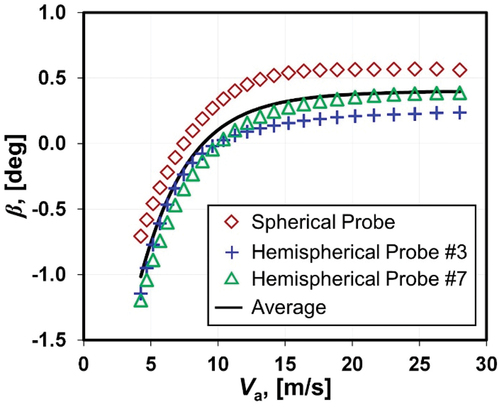
Since NIST’s wind tunnel produces nearly axial flow in its test section, both β and α are close to, but not exactly, zero due to growing boundary layers along the tunnel walls. To develop the calibration functions f_β and f_α, the yaw (β) and pitch (α) angles of the flow in the test section must be measured with respect to the tunnel’s axis. The authors used three different 5-hole probes (hemispherical probe #3, hemispherical probe #7, and a spherical probe) to measure β in the test section as a function of velocity over the range 4.25 m/s ≤ V_a≤ 28 m/s. After installing each 5-hole probe in the wind tunnel and establishing a constant airspeed V_a = 4.25 m/s, the authors used the automated traverse system to adjust β_p until the yaw pressure equaled zero, (p₂₃ = 0). At each subsequent velocity set point the authors again adjusted β_p until p₂₃ = 0. Figure 7 shows the measured yaw angles for all three probes. For each probe, β monotonically increased up to V_a ≈15 m/s and then tended toward a fixed value. The authors suspect that the differences between the three probes resulted from imperfect symmetry of the probes’ yaw pressure ports. The average yaw angle of the three 5-hole probes (β_avg) is indicated by the solid line (──) in Figure 7. The authors used β_avg to calculate βʹ = β_avg - β_p, and subsequently to determine the calibration curve f_β. The authors modeled the uncertainty as a rectangular distribution equal to u_axial(β) = 0.31 °/$\sqrt{3}$, where 0.31 ° is the largest, absolute deviation from β_avg.

Figure 7. Plot of the measured yaw angle β versus the axial velocity V_a in NIST’s wind tunnel test section.

In NIST’s wind tunnel, the authors expect that the magnitude of the off-axis pitch flow is comparable to the off-axis yaw flow; however, the authors did not measure the α_p = 0 ° streamline. The maximum sensitivity of V_a to an error in either α or β occurs at their maximum measured values |α _max| = 20 ° or |β_max| = 45 °. Because α _max<< β_max, the maximum sensitivity of V_a to α is only 1/3^rd of that to β. [See Equation (12a)(12a) $U_{\mathrm{r}}(f{\upsilon }_{\mathrm{n}})=2{\left[\begin{array}{c}\frac{u_{\mathrm{r}}^2(\rho )}{4}+u_{\mathrm{r}}^2(V_{\mathrm{L}\mathrm{D}\mathrm{A}})+u_{\mathrm{r},\mathrm{R}\mathrm{e}\mathrm{s}\mathrm{i}\mathrm{d}}^2(f{\upsilon }_{\mathrm{n}})+{100}^2{tan}^2(\alpha { }^{\mathrm{\prime }})u^2(\alpha { }^{\mathrm{\prime }})\\ +{100}^2{tan}^2(\beta { }^{\mathrm{\prime }})u^2(\beta { }^{\mathrm{\prime }})+\frac{u_{\mathrm{r}}^2(p_{\mathrm{P}\mathrm{S}\mathrm{E}\mathrm{U}\mathrm{D}\mathrm{O}})}{4}+{100}^2\sum _{i=1}^5{\left(\frac{1}{f{\upsilon }_{\mathrm{n}}}\frac{\mathrm{\partial }f{\upsilon }_{\mathrm{n}}}{\mathrm{\partial }{p}_{\mathrm{i}\mathrm{s}}}\right)}^2{u}^2(p_{\mathrm{i}\mathrm{s}})\end{array}\right]}^{1/2},$(12a) in Sect. 6.1.] The authors assumed that the pitch angle was zero (α = 0 °) and calculated the relative pitch angle by α ʹ = – α_p. Our estimate of the uncertainty of off-axis pitch flow is u_axial(α) = 0.5 °/$\sqrt{3}$ where 0.5 ° is the assumed to be the maximum off-axis pitch angle.

Calibration function for normal velocity

At each yaw and pitch orientation in Figure 6, the component of the air velocity normal to port #1 is

(9) $V_{\mathrm{n}}=V_{\mathrm{L}\mathrm{D}\mathrm{A}}cos\beta { }^{\mathrm{\prime }}cos\alpha { }^{\mathrm{\prime }}.$(9)

The normal velocity V_n is analogous to the expression for the stack axial velocity V_a in Equation (1)(1) $V_{\mathrm{a}}=Vcos\beta cos\alpha .$(1) . That is, measuring V_n in the (X ʹ, Y ʹ, Z ʹ) reference frame in Figure 6 is analogous to measuring V_a in a stack’s (X, Y, Z) reference frame in Figure 1. For this reason, V_n is the key calibration parameter for non-nulling stack flow measurements.

The authors derive Equation (9)(9) $V_{\mathrm{n}}=V_{\mathrm{L}\mathrm{D}\mathrm{A}}cos\beta { }^{\mathrm{\prime }}cos\alpha { }^{\mathrm{\prime }}.$(9) by taking the inner product V ∙ $\hat{n}$ of wind tunnel velocity V = V_LDAî and the unit normal vector in Figure 6, $\hat{n}$ = cosβ_p cosα_p î - sinα_p cosβ_p ĵ +sinβ_p $\stackrel{\mathbf{ˆ}}{\mathbf{k}}$. The result is V_n = V_LDA cosβ_p cosα_p. Substituting β_p = β - βʹ and α_p= α - α ʹ from Equation 8(8a) $\beta { }^{\mathrm{\prime }}=\beta -{\beta }_p,$(8a) (a,b) into the normal velocity results in V_n = V_LDA cos(βʹ - β) cos(α ʹ - α). Here, the authors switched the polarity of angles since cos(β - βʹ) = cos(βʹ - β) and cos(α - αʹ) = cos(α ʹ - α). The resulting expression for the normal velocity is identical to Equation (9)(9) $V_{\mathrm{n}}=V_{\mathrm{L}\mathrm{D}\mathrm{A}}cos\beta { }^{\mathrm{\prime }}cos\alpha { }^{\mathrm{\prime }}.$(9) provided the flow in wind tunnel has zero yaw and pitch angles, β = 0 ° and α = 0 °. If the yaw and pitch angles are not identically zero, one can correct for the departure from axial flow by measuring the β_p = 0 ° and α_p = 0 ° streamlines as the authors did for the yaw streamline in Section 5.6. Any remaining deviations from axial flow due to the yaw or pitch angles are included in the uncertainty budget (See Section 6).

In what follows the measurements and calculated uncertainties of V_n, α ʹ, and βʹ in the (X ʹ, Y ʹ, Z ʹ) reference frame in Figure 6 directly correspond to measurements of V_a, α, and β in the stack’s (X, Y, Z) reference in Figure 1. However, for consistency with the preceding sections the authors continue to specify the calibration domain and the applicable domain of the calibration curves using α and β instead of α ʹ, and βʹ.

To facilitate straightforward non-nulling velocity measurements, the authors define the normal velocity calibration factor,

(10) ${\upsilon }_{\mathrm{n}}=\frac{V_{\mathrm{n}}}{V_{\mathrm{P}\mathrm{S}\mathrm{E}\mathrm{U}\mathrm{D}\mathrm{O}}}=\sqrt{r_{\mathrm{d}\mathrm{y}\mathrm{n}}}cos\beta { }^{\mathrm{\prime }}cos\alpha { }^{\mathrm{\prime }}.$(10)

This dimensionless calibration factor is the ratio of the normal velocity in Equation (9)(9) $V_{\mathrm{n}}=V_{\mathrm{L}\mathrm{D}\mathrm{A}}cos\beta { }^{\mathrm{\prime }}cos\alpha { }^{\mathrm{\prime }}.$(9) and the pseudo velocity defined by

(11) $V_{\mathrm{P}\mathrm{S}\mathrm{E}\mathrm{U}\mathrm{D}\mathrm{O}}=\sqrt{2p_{\mathrm{P}\mathrm{S}\mathrm{E}\mathrm{U}\mathrm{D}\mathrm{O}}/\rho }.$(11)

Here, the LDA velocity in Equation (9)(9) $V_{\mathrm{n}}=V_{\mathrm{L}\mathrm{D}\mathrm{A}}cos\beta { }^{\mathrm{\prime }}cos\alpha { }^{\mathrm{\prime }}.$(9) is replaced by V_LDA = $\sqrt{2p_{dyn}/\rho }$. A calibration curve for the normal velocity is obtained by replacing βʹ, α ʹ, and r_dyn, in Equation (10)(10) ${\upsilon }_{\mathrm{n}}=\frac{V_{\mathrm{n}}}{V_{\mathrm{P}\mathrm{S}\mathrm{E}\mathrm{U}\mathrm{D}\mathrm{O}}}=\sqrt{r_{\mathrm{d}\mathrm{y}\mathrm{n}}}cos\beta { }^{\mathrm{\prime }}cos\alpha { }^{\mathrm{\prime }}.$(10) with the three calibration curves f_β, f_α, and f_rdyn to obtain Equation (5)(5) $f{\upsilon }_{\mathrm{n}}=\sqrt{f_{\mathrm{r}\mathrm{d}\mathrm{y}\mathrm{n}}}cos{f}_{\beta }cos{f}_{\alpha }.$(5) given earlier in Section 3.3.

Calibration and verification data

The authors calibrated all 7 hemispherical probes using the 130-point quasi-random data collection strategy discussed in Section 3.3. The calibration domain was |α | ≤ 20 °; |β | ≤ 45 °; 4.5 m/s ≤ V_a≤27 m/s. The 130 calibration set points were used to develop the calibration curves f_α, f_β, f_rdyn, and f_r1s. The authors used these calibration curves to calculate fυ_n as specified by Equation (5)(5) $f{\upsilon }_{\mathrm{n}}=\sqrt{f_{\mathrm{r}\mathrm{d}\mathrm{y}\mathrm{n}}}cos{f}_{\beta }cos{f}_{\alpha }.$(5) .

For probe #3 the authors collected 1200 additional points over a 3-month period, herein referred to as verification data. The values of α, β, and V_a selected for the verification data differed from each other and from the values used for the 130-point calibration. The authors computed fit residuals for the 130-point calibration and for the 1200-point verification data using 100 (f υ_n / υ_n − 1). The calibration fit residuals indicated how well the calibration curve f υ_n represents the 130 measurements of υ_n. On the other hand, the verification residuals indicated if f υ_n is accurately described using only 130 points.

Figure 8 shows these residuals plotted against the axial velocity V_a measured by the LDA for probe #3. The residuals of the 130 calibration set points are denoted by the circles (●). More than 95% of the calibration residuals (●) lie within the expanded uncertainty U_r(fυ_n) = ±1.53% indicated by the dashed lines (——). Section 6 is a detailed discussion of U_r(fυ_n).

Figure 8. The residuals of the normal velocity calibration factor fυ_n vs the axial velocity V_LDA measured by the LDA. Using a regression analysis of the 130 measured υ_n’s the authors developed a third degree polynomial fυ_n(r₁₂, r₂₃, r₄₅) for υ_n. The circles (●) are the residuals from the polynomial and the dashed lines at ±1.53% indicate the expanded uncertainty U_r(fυ_n) of the 130 υ_n points. The squares (

) and crosses (×) represent the residuals of independently-measured verification points from the same polynomial for |β_p| ≤ 40 ° and for 40 ° ≤ |β_p| ≤ 45 °, respectively.

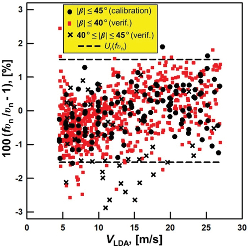
In Figure 8, the residuals of the 1200 verification data points are separated into two groups denoted by squares () for values of |β | ≤ 40 ° and by crosses (×) for values of 40 ° < |β | ≤ 45 °. Only 3.5% of the 1108 squares are outside the expanded uncertainty limits calculated using the calibration data. However, 26% of the crosses are outside the uncertainty limits. Thus, to ensure 95% of the residuals are within the uncertainty limits, the non-nulling method should not be used over the entire calibration domain. The applicable domain excludes |β | > 40 °.

In Figure 8, the excellent overlap of the calibration and verification residuals is evidence of the stability of probe #3 because verification data were acquired 3 months after the 130-point calibration data. Also in Figure 8, the small positive slope of both the calibration and verification residuals is evidence that the calibration factor fυ_n has a weak Reynolds number dependence. This slope could be removed by introducing additional Re-dependent terms into fυ_n. However, lower uncertainties cannot be realized in field applications because the values of the Re-dependent terms might depend on the level of the turbulence intensity, which is generally unknown in stacks.

In this analysis the fυ_n calibration curve consisted of a 3^rd degree polynomial of the three pressure ratios in Equation (4c)(4c) $\begin{array}{rl}& r_{12}=p_{12}/p_{\mathrm{P}\mathrm{S}\mathrm{E}\mathrm{U}\mathrm{D}\mathrm{O}},\\ & r_{23}=p_{23}/p_{\mathrm{P}\mathrm{S}\mathrm{E}\mathrm{U}\mathrm{D}\mathrm{O}},\\ & r_{45}=p_{45}/p_{\mathrm{P}\mathrm{S}\mathrm{E}\mathrm{U}\mathrm{D}\mathrm{O}}.\end{array}$(4c) . When the authors repeated the analysis using a 4^th degree polynomial, the uncertainty of the fit residuals reduced by a factor of 1.49 and lead to a lower expanded uncertainty equal of 1.19% of fυ_n. However, only 83. 5% of the |β | ≤ 40 ° verification data lie within the uncertainty limits, indicating poor reproducibility. The authors are not certain what caused the irreproducibility observed for the 4^th degree polynomial fit, and additional reproducibility studies are necessary.

Uncertainty analysis

The authors developed the calibration curves fυ_n, f_β, f_α, and f_r1s using NIST’s wind tunnel, differential pressure ssensors, and the LDA system that NIST routinely uses to calibrate external customers’ wind speed instruments. In this section the authors provide sample uncertainty calculations of the calibration curves for probe #3. The calculated uncertainties are valid for velocities ranging from 4.5 m/s ≤ V_a≤ 27 m/s and pitch and yaw angles from |α| ≤ 20 ° and |β| ≤ 40 °, respectively. The authors used the method of propagation of uncertainty (Coleman and Steele 1999; International Organization for Standardization 1996; Taylor and Kuyatt 0000) and determined the expanded uncertainty of the four of calibration curves: 1) U_r(fυ_n) = 1.53% calculated using Equation (12a)(12a) $U_{\mathrm{r}}(f{\upsilon }_{\mathrm{n}})=2{\left[\begin{array}{c}\frac{u_{\mathrm{r}}^2(\rho )}{4}+u_{\mathrm{r}}^2(V_{\mathrm{L}\mathrm{D}\mathrm{A}})+u_{\mathrm{r},\mathrm{R}\mathrm{e}\mathrm{s}\mathrm{i}\mathrm{d}}^2(f{\upsilon }_{\mathrm{n}})+{100}^2{tan}^2(\alpha { }^{\mathrm{\prime }})u^2(\alpha { }^{\mathrm{\prime }})\\ +{100}^2{tan}^2(\beta { }^{\mathrm{\prime }})u^2(\beta { }^{\mathrm{\prime }})+\frac{u_{\mathrm{r}}^2(p_{\mathrm{P}\mathrm{S}\mathrm{E}\mathrm{U}\mathrm{D}\mathrm{O}})}{4}+{100}^2\sum _{i=1}^5{\left(\frac{1}{f{\upsilon }_{\mathrm{n}}}\frac{\mathrm{\partial }f{\upsilon }_{\mathrm{n}}}{\mathrm{\partial }{p}_{\mathrm{i}\mathrm{s}}}\right)}^2{u}^2(p_{\mathrm{i}\mathrm{s}})\end{array}\right]}^{1/2},$(12a) , 2(2) $V=\sqrt{2p_{\mathrm{d}\mathrm{y}\mathrm{n}}/\rho }.$(2) ) U(f_β) = 0.86 ° calculated using Equation (12b)(12b) $U(f_{\beta })=2\sqrt{u^2({\beta }_{\mathrm{p}})+u_{\mathrm{a}\mathrm{x}\mathrm{i}\mathrm{a}\mathrm{l}}^2(\beta )+u_{\mathrm{R}\mathrm{e}\mathrm{s}\mathrm{i}\mathrm{d}}^2(f_{\beta })+\sum _{i=1}^5{\left(\frac{\mathrm{\partial }{f}_{\beta }}{\mathrm{\partial }{p}_{\mathrm{i}\mathrm{s}}}\right)}^2{u}^2(p_{\mathrm{i}\mathrm{s}})}$(12b) , 3(3) $p_{\mathrm{P}\mathrm{S}\mathrm{E}\mathrm{U}\mathrm{D}\mathrm{O}}=\sqrt{p_{12}^2+p_{13}^2+p_{14}^2+p_{15}^2},$(3) ) U(f_α) = 0.96 ° calculated using Equation (12c)(12c) $U(f_{\alpha })=2\sqrt{\begin{array}{c}{u}^2({\alpha }_{\text{p}})+u_{\text{axial}}^2(\alpha )\\ +u_{\text{Resid}}^2(f_{\alpha })\\ +{\displaystyle \sum _{i=1}^5{\left(\frac{\partial f_{\alpha }}{\partial p_{\text{is}}}\right)}^2{u}^2(p_{\text{is}})}\end{array}}$(12c) , and 4) U(f_r1s) = 0.011 calculated using Equation (12d)(12d) $U(f_{\mathrm{r}1\mathrm{s}})=2\sqrt{u_{\mathrm{R}\mathrm{e}\mathrm{s}\mathrm{i}\mathrm{d}}^2(f_{\mathrm{r}1\mathrm{s}})+\sum _{n=1}^5{\left(\frac{\mathrm{\partial }{\mathrm{r}}_{1\mathrm{s}}}{\mathrm{\partial }{p}_{\mathrm{n}\mathrm{s}}}\right)}^2{u}^2(p_{\mathrm{n}\mathrm{s}})+\sum _{n=1}^5{\left(\frac{\mathrm{\partial }{f}_{\mathrm{r}1\mathrm{s}}}{\mathrm{\partial }{p}_{\mathrm{n}\mathrm{s}}}\right)}^2{u}^2(p_{\mathrm{n}\mathrm{s}})}$(12d) .

Our uncertainty analysis indicates that the uncertainty of NIST’s instruments was not the largest uncertainty source. For example, the last term in Equations (12a)(12a) $U_{\mathrm{r}}(f{\upsilon }_{\mathrm{n}})=2{\left[\begin{array}{c}\frac{u_{\mathrm{r}}^2(\rho )}{4}+u_{\mathrm{r}}^2(V_{\mathrm{L}\mathrm{D}\mathrm{A}})+u_{\mathrm{r},\mathrm{R}\mathrm{e}\mathrm{s}\mathrm{i}\mathrm{d}}^2(f{\upsilon }_{\mathrm{n}})+{100}^2{tan}^2(\alpha { }^{\mathrm{\prime }})u^2(\alpha { }^{\mathrm{\prime }})\\ +{100}^2{tan}^2(\beta { }^{\mathrm{\prime }})u^2(\beta { }^{\mathrm{\prime }})+\frac{u_{\mathrm{r}}^2(p_{\mathrm{P}\mathrm{S}\mathrm{E}\mathrm{U}\mathrm{D}\mathrm{O}})}{4}+{100}^2\sum _{i=1}^5{\left(\frac{1}{f{\upsilon }_{\mathrm{n}}}\frac{\mathrm{\partial }f{\upsilon }_{\mathrm{n}}}{\mathrm{\partial }{p}_{\mathrm{i}\mathrm{s}}}\right)}^2{u}^2(p_{\mathrm{i}\mathrm{s}})\end{array}\right]}^{1/2},$(12a) through (12d) account for the uncertainty in each of the non-nulling calibration curves due to measurement errors in the differential pressures p_1s, p_2s, p_3s, p_4s, and p_5s. These uncertainties were negligible and accounted for less than 1% of each calibration curve’s uncertainty budget. Likewise, the uncertainty attributed to the density measurement made a negligible contribution to the fυ_n uncertainty budget, and the measurement uncertainty of the LDA velocity only made a modest contribution (i.e., less than 8.4%). The dominant uncertainty source for all the calibration curves is attributed to the fit residuals of the 3 variable, 3^rd degree polynomial fit used to model the wind tunnel data. As a result, low uncertainty non-nulling calibrations do not require laboratory grade pressure sensors or state-of-the anemometers. The authors expect that laboratories implementing this non-nulling protocol can generate calibration curves with expanded uncertainties to achieve U_r(fυ_n) ≤ 2%; U(f_β) ≤ 1 °; U(f_α) ≤ 1 °, and U(f_r1s) ≤ 0.1 using selected industrial-grade differential pressure transducers and anemometers.

Because this manuscript is intended to support an ASME documentary standard on non-nulling methods, the authors provide a comprehensive uncertainty analysis that accounts for all the uncertainty components including those that are negligible in the NIST analysis. In this way, stack laboratories implementing the non-nulling method can assess the uncertainty for a sensor calibration using their air speed instrumentation.

Uncertainty of the normal velocity calibration factor

For stack flow applications the most important calibration curve is fυ_n since it directly corresponds to the stack axial velocity via Equation (15a)(15a) $V_{\mathrm{a},\mathrm{N}\mathrm{N}}=V_{\mathrm{P}\mathrm{S}\mathrm{E}\mathrm{U}\mathrm{D}\mathrm{O}}f{\upsilon }_{\mathrm{n}}{C}_{\beta }{C}_{\alpha },$(15a) . The expanded uncertainty of fυ_n is

(12a) $U_{\mathrm{r}}(f{\upsilon }_{\mathrm{n}})=2{\left[\begin{array}{c}\frac{u_{\mathrm{r}}^2(\rho )}{4}+u_{\mathrm{r}}^2(V_{\mathrm{L}\mathrm{D}\mathrm{A}})+u_{\mathrm{r},\mathrm{R}\mathrm{e}\mathrm{s}\mathrm{i}\mathrm{d}}^2(f{\upsilon }_{\mathrm{n}})+{100}^2{tan}^2(\alpha { }^{\mathrm{\prime }})u^2(\alpha { }^{\mathrm{\prime }})\\ +{100}^2{tan}^2(\beta { }^{\mathrm{\prime }})u^2(\beta { }^{\mathrm{\prime }})+\frac{u_{\mathrm{r}}^2(p_{\mathrm{P}\mathrm{S}\mathrm{E}\mathrm{U}\mathrm{D}\mathrm{O}})}{4}+{100}^2\sum _{i=1}^5{\left(\frac{1}{f{\upsilon }_{\mathrm{n}}}\frac{\mathrm{\partial }f{\upsilon }_{\mathrm{n}}}{\mathrm{\partial }{p}_{\mathrm{i}\mathrm{s}}}\right)}^2{u}^2(p_{\mathrm{i}\mathrm{s}})\end{array}\right]}^{1/2},$(12a)

where u_r,Resid(fυ_n) = 0.67% is the standard deviation of curve fit residuals (See Figure 8). This uncertainty makes the largest contribution to the uncertainty budget, ranging from 51% to 88% of U_r(fυ_n) depending on the values of α ʹ and βʹ. The circles () in Figure 9 show the contribution of u_r,Resid(fυ_n) to the uncertainty budget as a function of βʹ. At any value of βʹ, the corresponding uncertainty components that are specified in Equation (12a)(12a) $U_{\mathrm{r}}(f{\upsilon }_{\mathrm{n}})=2{\left[\begin{array}{c}\frac{u_{\mathrm{r}}^2(\rho )}{4}+u_{\mathrm{r}}^2(V_{\mathrm{L}\mathrm{D}\mathrm{A}})+u_{\mathrm{r},\mathrm{R}\mathrm{e}\mathrm{s}\mathrm{i}\mathrm{d}}^2(f{\upsilon }_{\mathrm{n}})+{100}^2{tan}^2(\alpha { }^{\mathrm{\prime }})u^2(\alpha { }^{\mathrm{\prime }})\\ +{100}^2{tan}^2(\beta { }^{\mathrm{\prime }})u^2(\beta { }^{\mathrm{\prime }})+\frac{u_{\mathrm{r}}^2(p_{\mathrm{P}\mathrm{S}\mathrm{E}\mathrm{U}\mathrm{D}\mathrm{O}})}{4}+{100}^2\sum _{i=1}^5{\left(\frac{1}{f{\upsilon }_{\mathrm{n}}}\frac{\mathrm{\partial }f{\upsilon }_{\mathrm{n}}}{\mathrm{\partial }{p}_{\mathrm{i}\mathrm{s}}}\right)}^2{u}^2(p_{\mathrm{i}\mathrm{s}})\end{array}\right]}^{1/2},$(12a) sum to 100%. The authors calculate the contribution of each component by $100S_{\mathrm{i}}^2{u}_{\mathrm{r}}^2(x_{\mathrm{i}})/\sum S_{\mathrm{i}}^2{u}_{\mathrm{r}}^2(x_{\mathrm{i}})$ where u_r(x_i) is the relative standard uncertainty of the i^th component and $S_{\mathrm{i}}=\frac{x_{\mathrm{i}}}{{\upsilon }_{\mathrm{n}}}\frac{\mathrm{\partial }{\upsilon }_{\mathrm{n}}}{\mathrm{\partial }{x}_{\mathrm{i}}}$ is its corresponding normalized sensitivity coefficient.

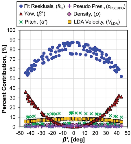
Figure 9. Percent contribution of the uncertainty components of U_r(fυ_n) in Equation (12a)(12a) $U_{\mathrm{r}}(f{\upsilon }_{\mathrm{n}})=2{\left[\begin{array}{c}\frac{u_{\mathrm{r}}^2(\rho )}{4}+u_{\mathrm{r}}^2(V_{\mathrm{L}\mathrm{D}\mathrm{A}})+u_{\mathrm{r},\mathrm{R}\mathrm{e}\mathrm{s}\mathrm{i}\mathrm{d}}^2(f{\upsilon }_{\mathrm{n}})+{100}^2{tan}^2(\alpha { }^{\mathrm{\prime }})u^2(\alpha { }^{\mathrm{\prime }})\\ +{100}^2{tan}^2(\beta { }^{\mathrm{\prime }})u^2(\beta { }^{\mathrm{\prime }})+\frac{u_{\mathrm{r}}^2(p_{\mathrm{P}\mathrm{S}\mathrm{E}\mathrm{U}\mathrm{D}\mathrm{O}})}{4}+{100}^2\sum _{i=1}^5{\left(\frac{1}{f{\upsilon }_{\mathrm{n}}}\frac{\mathrm{\partial }f{\upsilon }_{\mathrm{n}}}{\mathrm{\partial }{p}_{\mathrm{i}\mathrm{s}}}\right)}^2{u}^2(p_{\mathrm{i}\mathrm{s}})\end{array}\right]}^{1/2},$(12a) . The figure shows the uncertainty contribution from the polynomial fit residuals u_r,Resid(fυ_n) dominate the uncertainty budget.

The terms $u(\alpha { }^{\mathrm{\prime }})=\sqrt{u^2({\alpha }_{\mathrm{p}})+u_{\mathrm{a}\mathrm{x}\mathrm{i}\mathrm{a}\mathrm{l}}^2(\alpha )}$ and $u(\beta { }^{\mathrm{\prime }})=\sqrt{u^2({\beta }_{\mathrm{p}})+u_{\mathrm{a}\mathrm{x}\mathrm{i}\mathrm{a}\mathrm{l}}^2(\beta )}$ are uncertainties in the pitch and yaw angles. Although both uncertainties u(α ʹ) = 0.45 ° and u(βʹ) = 0.31 ° are fixed, their respective sensitivity coefficients, tan(α ʹ) and tan(βʹ), are variables that depend on the pitch and yaw angles. Since the authors calibrated the hemispherical probe over pitch angles ranging from −20 ° ≤ αʹ ≤ 20 ° while the yaw angle range −45 ° ≤ βʹ ≤ 45 ° was significantly larger, the maximum value of the pitch sensitivity coefficient is less than the maximum value of the yaw angle sensitivity coefficient, tan(20 °) < tan(45 °). Figure 9 illustrates this point. The yaw angle uncertainty denoted by the triangles () scale with tan²(βʹ) and accounts for 15% to 36.5% of uncertainty budget for |βʹ| > 30 °. In this region, the yaw angle is the second largest contributor to the uncertainty budget. The pitch angle uncertainty indicated by the crosses () makes a 10% to 14.5% contribution to the uncertainty budget when |αʹ| ≥ 15 ° and a negligible contribution at smaller pitch angles.

The uncertainties attributed to the LDA velocity and the air density measurements are u_r(V_LDA) = 0.205% and u_r(ρ) = 0.22%, respectively. The LDA contribution to the uncertainty budget denoted by the squares () ranges from 5% to 8.4% while the density contribution indicated by the diamonds () contributes less than to 2.4% since u_r(ρ) is reduced by its sensitivity coefficient $S_{\rho }^2=1/4$ as shown in Equation (12a)(12a) $U_{\mathrm{r}}(f{\upsilon }_{\mathrm{n}})=2{\left[\begin{array}{c}\frac{u_{\mathrm{r}}^2(\rho )}{4}+u_{\mathrm{r}}^2(V_{\mathrm{L}\mathrm{D}\mathrm{A}})+u_{\mathrm{r},\mathrm{R}\mathrm{e}\mathrm{s}\mathrm{i}\mathrm{d}}^2(f{\upsilon }_{\mathrm{n}})+{100}^2{tan}^2(\alpha { }^{\mathrm{\prime }})u^2(\alpha { }^{\mathrm{\prime }})\\ +{100}^2{tan}^2(\beta { }^{\mathrm{\prime }})u^2(\beta { }^{\mathrm{\prime }})+\frac{u_{\mathrm{r}}^2(p_{\mathrm{P}\mathrm{S}\mathrm{E}\mathrm{U}\mathrm{D}\mathrm{O}})}{4}+{100}^2\sum _{i=1}^5{\left(\frac{1}{f{\upsilon }_{\mathrm{n}}}\frac{\mathrm{\partial }f{\upsilon }_{\mathrm{n}}}{\mathrm{\partial }{p}_{\mathrm{i}\mathrm{s}}}\right)}^2{u}^2(p_{\mathrm{i}\mathrm{s}})\end{array}\right]}^{1/2},$(12a) . The last two uncertainty components in Equation (12a)(12a) $U_{\mathrm{r}}(f{\upsilon }_{\mathrm{n}})=2{\left[\begin{array}{c}\frac{u_{\mathrm{r}}^2(\rho )}{4}+u_{\mathrm{r}}^2(V_{\mathrm{L}\mathrm{D}\mathrm{A}})+u_{\mathrm{r},\mathrm{R}\mathrm{e}\mathrm{s}\mathrm{i}\mathrm{d}}^2(f{\upsilon }_{\mathrm{n}})+{100}^2{tan}^2(\alpha { }^{\mathrm{\prime }})u^2(\alpha { }^{\mathrm{\prime }})\\ +{100}^2{tan}^2(\beta { }^{\mathrm{\prime }})u^2(\beta { }^{\mathrm{\prime }})+\frac{u_{\mathrm{r}}^2(p_{\mathrm{P}\mathrm{S}\mathrm{E}\mathrm{U}\mathrm{D}\mathrm{O}})}{4}+{100}^2\sum _{i=1}^5{\left(\frac{1}{f{\upsilon }_{\mathrm{n}}}\frac{\mathrm{\partial }f{\upsilon }_{\mathrm{n}}}{\mathrm{\partial }{p}_{\mathrm{i}\mathrm{s}}}\right)}^2{u}^2(p_{\mathrm{i}\mathrm{s}})\end{array}\right]}^{1/2},$(12a) are the pseudo dynamic pressure p_pseudo indicated by the crosses () and the uncertainty in the fυ_n calibration curve due to the uncertainty in the differential pressure measurements. The contributions of both terms are negligible relative to U_r(fυ_n).

Finally, the authors point out that the expanded uncertainty U_r(fυ_n) plotted in Figure 8 is an approximation. For simplicity, this plot used the average values of the pitch and yaw uncertainties at each velocity so that U_r(fυ_n), which depends on V_a, αʹ, and βʹ could be conveniently plotted as a function of V_a alone.

Uncertainty of the yaw angle calibration curve

The authors used a 3 variable, 3^rd degree polynomial f_β fitted to measured values of the relative yaw angle βʹ. The authors plotted the residuals of the calibration curve f_β - βʹ versus the velocity measured by the LDA in Figure 10a. The residuals for the calibration curves f_α and f_r1s use similar notation and are denoted by f_α - α ʹ and f_r1s - r_1s, respectively. The triangles () in Figure 10a show the residuals of the yaw angle calibration curve f_β, and the dashed lines (----) indicate its expanded uncertainty. The expanded uncertainty is expressed by

Figure 10. Residuals of the respective calibration curves f_β, f_α, and f_r1s plotted versus the axial velocity V_a measured by the LDA working standard. The dashed lines (----) indicate expanded uncertainty of the respective calibration curves. (a) Residuals of f_β indicated by triangles (

); (b) Residuals of f_α indicated by circles (

); (c) Residuals of f_r1s indicated by squares (

).

(12b) $U(f_{\beta })=2\sqrt{u^2({\beta }_{\mathrm{p}})+u_{\mathrm{a}\mathrm{x}\mathrm{i}\mathrm{a}\mathrm{l}}^2(\beta )+u_{\mathrm{R}\mathrm{e}\mathrm{s}\mathrm{i}\mathrm{d}}^2(f_{\beta })+\sum _{i=1}^5{\left(\frac{\mathrm{\partial }{f}_{\beta }}{\mathrm{\partial }{p}_{\mathrm{i}\mathrm{s}}}\right)}^2{u}^2(p_{\mathrm{i}\mathrm{s}})}$(12b)

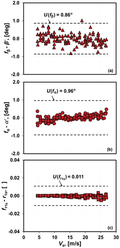
where u(β_p) = 0.25 ° is the uncertainty in the probe’s yaw angle orientation, u_axial(β) = 0.31 °/$\sqrt{3}$ is the uncertainty attributed to a non-zero yaw angle of the velocity in the wind tunnel test section, and u_Resid(f_β) = 0.315 ° is the standard deviation of curve fit residuals. The last term in Equation (12b)(12b) $U(f_{\beta })=2\sqrt{u^2({\beta }_{\mathrm{p}})+u_{\mathrm{a}\mathrm{x}\mathrm{i}\mathrm{a}\mathrm{l}}^2(\beta )+u_{\mathrm{R}\mathrm{e}\mathrm{s}\mathrm{i}\mathrm{d}}^2(f_{\beta })+\sum _{i=1}^5{\left(\frac{\mathrm{\partial }{f}_{\beta }}{\mathrm{\partial }{p}_{\mathrm{i}\mathrm{s}}}\right)}^2{u}^2(p_{\mathrm{i}\mathrm{s}})}$(12b) accounts for the uncertainty in the f_β calibration curve attributed to uncertainty in the differential pressure measurements. This term makes an insignificant contribution to the f_β uncertainty budget.

Uncertainty of the pitch angle calibration curve

Figure 10b shows the residuals () of the f_α calibration curve, and its expanded uncertainty indicated by the dashed lines (----). The expanded uncertainty is calculated by

(12c) $U(f_{\alpha })=2\sqrt{\begin{array}{c}{u}^2({\alpha }_{\text{p}})+u_{\text{axial}}^2(\alpha )\\ +u_{\text{Resid}}^2(f_{\alpha })\\ +{\displaystyle \sum _{i=1}^5{\left(\frac{\partial f_{\alpha }}{\partial p_{\text{is}}}\right)}^2{u}^2(p_{\text{is}})}\end{array}}$(12c)

where only the first three terms make a significant contribution to the uncertainty budget. Here, u(α_p) = 0.35 ° is the uncertainty attributed to the probe’s pitch orientation; u_axial(α) = 0.5 °/$\sqrt{3}$ is the uncertainty attributed to a non-zero pitch angle of the velocity in the wind tunnel test section; and u_Resid(f_α) = 0.155 ° is the standard deviation of curve fit residuals.

Uncertainty of the static pressure parameter calibration curve

The residuals of the f_r1s calibration curve are denoted by the squares () in Figure 10c, and the dashed lines (----) show the expanded uncertainty. The expanded uncertainty is calculated by

(12d) $U(f_{\mathrm{r}1\mathrm{s}})=2\sqrt{u_{\mathrm{R}\mathrm{e}\mathrm{s}\mathrm{i}\mathrm{d}}^2(f_{\mathrm{r}1\mathrm{s}})+\sum _{n=1}^5{\left(\frac{\mathrm{\partial }{\mathrm{r}}_{1\mathrm{s}}}{\mathrm{\partial }{p}_{\mathrm{n}\mathrm{s}}}\right)}^2{u}^2(p_{\mathrm{n}\mathrm{s}})+\sum _{n=1}^5{\left(\frac{\mathrm{\partial }{f}_{\mathrm{r}1\mathrm{s}}}{\mathrm{\partial }{p}_{\mathrm{n}\mathrm{s}}}\right)}^2{u}^2(p_{\mathrm{n}\mathrm{s}})}$(12d)

where only the curve fit residual expressed by the first term u_Resid(f_r1s) = 0.0054 Pa makes a significant contribution to the uncertainty.

Uncertainty of the air density

The uncertainty in the wind tunnel air density is calculated by applying the propagation of uncertainty to the air density correlation in Equation (7)(7) $\rho =c_0/T\left[p_s-c_{1}RHexp\left(-c_2/T\right)\right].$(7) to obtain

(13) $u_{\mathrm{r}}(\rho )={\left[\begin{array}{c}{u}_{\mathrm{r},\mathrm{E}\mathrm{O}\mathrm{S}}^2(\rho )+{\left(\frac{p_{\mathrm{s}}{c}_0}{\rho T}\right)}^2{u}_{\mathrm{r}}^2(p_{\mathrm{s}})+{100}^2{\left(\frac{c_0{c}_{1}exp(-c_2/T)}{\rho T}\right)}^2{u}^2(RH)\\ +{100}^2{\left(\frac{1}{T}\right)}^2{\left[1+\left(\frac{c_2}{T}\right)\left(\frac{p_{\mathrm{s}}{c}_0}{\rho T}-1\right)\right]}^2{u}^2(T)\end{array}\right]}^{1/2}.$(13)

where u_r(p_s) = 0.05% is the relative static pressure uncertainty; u(T) = 0.5 K is the temperature uncertainty; and u(RH) = 2.5% is the uncertainty in relative humidity (in the units % relative humidity). The resulting uncertainty is u_r(ρ) = 0.22%. Figure 9 shows that u_r(ρ) is negligible relative to u_r(fυ_n) indicating that highly accurate density measurements are not necessary to achieve U_r(fυ_n) ≤ 2%.

Uncertainty of the differential pressure measurements

During probe calibrations, the authors measured the pressure at each port relative to the wind tunnel static pressure, p_1s, p_2s, p_3s, p_4s, and p_5s, using five 698A Baratron heated, high accuracy, bidirectional differential capacitance manometers with full scale of 10 Torr.² NIST’s calibration records indicate that the standard uncertainty of each differential pressure transducer is u_r,cal(p_is) = 0.1% of reading from 9 Pa to 666.7 Pa and u_cal(p_is) = 0.009 Pa below 9 Pa. The authors zeroed each manometer at the start of each calibration. A conservative estimate of the standard uncertainty attributed to zero drift is u_zero(p_is) = 0.002 Pa. The uncertainty of the differential pressure is

(14) $u(p_{\mathrm{i}\mathrm{s}})=\sqrt{u_{\mathrm{c}\mathrm{a}\mathrm{l}}^2(p_{\mathrm{i}\mathrm{s}})+u_{\mathrm{z}\mathrm{e}\mathrm{r}\mathrm{o}}^2(p_{\mathrm{i}\mathrm{s}})},$(14)

for i = 1 to 5.

Applying calibration curves in stack flow measurements

In stack flow measurement applications the calibration curves fυ_n, f_β, f_α, and f_r1s are used to determine 1) the stack axial velocity V_a,NN in Equation (15a)(15a) $V_{\mathrm{a},\mathrm{N}\mathrm{N}}=V_{\mathrm{P}\mathrm{S}\mathrm{E}\mathrm{U}\mathrm{D}\mathrm{O}}f{\upsilon }_{\mathrm{n}}{C}_{\beta }{C}_{\alpha },$(15a) ; 2) the yaw angle β_NN in Equation (15b)(15b) ${\beta }_{\mathrm{N}\mathrm{N}}=f_{\beta }+{\beta }_{\mathrm{p}}.$(15b) ; 3) the pitch angle α_NN in Equation (15c)(15c) ${\alpha }_{\mathrm{N}\mathrm{N}}=f_{\alpha }+{\alpha }_{\mathrm{p}}.$(15c) ; and 4) the static pressure p_s,NN in Equation (15d)(15d) $p_{\mathrm{s},\mathrm{N}\mathrm{N}}=-f_{\mathrm{r}1\mathrm{s}}{p}_{\mathrm{P}\mathrm{S}\mathrm{E}\mathrm{U}\mathrm{D}\mathrm{O}}+p_{1,\mathrm{r}\mathrm{e}\mathrm{f}}+p_{\mathrm{r}\mathrm{e}\mathrm{f}},$(15d) . Here, the subscript “NN” indicates that the variables are calculated using the non-nulling calibration curves.

When a hemispherical probe is installed in a stack or duct (See Figure 1) and oriented at non-zero yaw and pitch angles, α_p≠ 0 ° and β_p≠ 0 °, the axial velocity at a traverse point is

(15a) $V_{\mathrm{a},\mathrm{N}\mathrm{N}}=V_{\mathrm{P}\mathrm{S}\mathrm{E}\mathrm{U}\mathrm{D}\mathrm{O}}f{\upsilon }_{\mathrm{n}}{C}_{\beta }{C}_{\alpha },$(15a)

where fυ_n is determined by Equation (5)(5) $f{\upsilon }_{\mathrm{n}}=\sqrt{f_{\mathrm{r}\mathrm{d}\mathrm{y}\mathrm{n}}}cos{f}_{\beta }cos{f}_{\alpha }.$(5) , C_β = cos(f_β + β_p)/cos(f_β) is the yaw angle cosine correction factor that accounts for a non-zero yaw orientation, and C_α = cos(f_α + α_p)/cos(f_α) is the pitch angle cosine correction factor that accounts for a non-zero pitch orientation.

The stack flow’s yaw angle is the sum of the yaw angle calculated by the f_β calibration curve and the probe’s yaw angle orientation,

(15b) ${\beta }_{\mathrm{N}\mathrm{N}}=f_{\beta }+{\beta }_{\mathrm{p}}.$(15b)

Similarly, the pitch angle is the sum of the pitch angle calculated by the f_α calibration curve and the probe’s pitch angle orientation,

(15c) ${\alpha }_{\mathrm{N}\mathrm{N}}=f_{\alpha }+{\alpha }_{\mathrm{p}}.$(15c)

The static pressure is calculated by

(15d) $p_{\mathrm{s},\mathrm{N}\mathrm{N}}=-f_{\mathrm{r}1\mathrm{s}}{p}_{\mathrm{P}\mathrm{S}\mathrm{E}\mathrm{U}\mathrm{D}\mathrm{O}}+p_{1,\mathrm{r}\mathrm{e}\mathrm{f}}+p_{\mathrm{r}\mathrm{e}\mathrm{f}},$(15d)

where p_ref is the barometric pressure outside the stack, and p_1,ref is the pressure difference between the probe’s port #1 and the reference barometric pressure. In stack applications, p_s,NN is used in conjunction with the flue gas temperature and composition to determine its density, which in turn is used to calculate the pseudo velocity V_PSEUDO in Equation (11)(11) $V_{\mathrm{P}\mathrm{S}\mathrm{E}\mathrm{U}\mathrm{D}\mathrm{O}}=\sqrt{2p_{\mathrm{P}\mathrm{S}\mathrm{E}\mathrm{U}\mathrm{D}\mathrm{O}}/\rho }.$(11) . The authors then used the velocity scale V_PSEUDO in Equation (15a)(15a) $V_{\mathrm{a},\mathrm{N}\mathrm{N}}=V_{\mathrm{P}\mathrm{S}\mathrm{E}\mathrm{U}\mathrm{D}\mathrm{O}}f{\upsilon }_{\mathrm{n}}{C}_{\beta }{C}_{\alpha },$(15a) to calculate the axial velocity V_a,NN.

Ideally, the non-nulling method is implemented with the probe oriented at α_p = 0 ° and β_p = 0 ° as shown in Figure 1. In this special case, Equations (15a)(15a) $V_{\mathrm{a},\mathrm{N}\mathrm{N}}=V_{\mathrm{P}\mathrm{S}\mathrm{E}\mathrm{U}\mathrm{D}\mathrm{O}}f{\upsilon }_{\mathrm{n}}{C}_{\beta }{C}_{\alpha },$(15a) through (15c(15c) ${\alpha }_{\mathrm{N}\mathrm{N}}=f_{\alpha }+{\alpha }_{\mathrm{p}}.$(15c) ) simplify. First, the cosine correction factors for yaw and pitch angles in Equation (15a)(15a) $V_{\mathrm{a},\mathrm{N}\mathrm{N}}=V_{\mathrm{P}\mathrm{S}\mathrm{E}\mathrm{U}\mathrm{D}\mathrm{O}}f{\upsilon }_{\mathrm{n}}{C}_{\beta }{C}_{\alpha },$(15a) are both unity, C_α = 1 and C_β = 1. In addition, the yaw and pitch angles in Equation 15(15a) $V_{\mathrm{a},\mathrm{N}\mathrm{N}}=V_{\mathrm{P}\mathrm{S}\mathrm{E}\mathrm{U}\mathrm{D}\mathrm{O}}f{\upsilon }_{\mathrm{n}}{C}_{\beta }{C}_{\alpha },$(15a) (b,c) equal the respective relative yaw and pitch angles calculated by the f_β and f_α calibration curves.

In practice, probes are usually installed in stacks oriented at zero pitch α_p = 0 °; however, it is not always practical to orient probes at a zero yaw angle (β_p≠ 0 °). First, during stack measurements the probe head and its support shaft shown in Figure 2 are extended by attaching a long steel shaft to facilitate traversing the probe across the (5 m to 10 m) diameter of the stack. The probe extension is equipped with a flat surface that is kept outside the stack and is used as a reference to measure the probe’s yaw angle orientation when the probe’s head is inside the stack. If the flat reference surface on the probe extension is offset from the zero yaw orientation of the probe head so that β_p≠ 0 °, Equations (15a)(15a) $V_{\mathrm{a},\mathrm{N}\mathrm{N}}=V_{\mathrm{P}\mathrm{S}\mathrm{E}\mathrm{U}\mathrm{D}\mathrm{O}}f{\upsilon }_{\mathrm{n}}{C}_{\beta }{C}_{\alpha },$(15a) through Equation (15c)(15c) ${\alpha }_{\mathrm{N}\mathrm{N}}=f_{\alpha }+{\alpha }_{\mathrm{p}}.$(15c) are used to account for the yaw angle offset when calculating the axial velocity, as required by EPA regulations (EPA 2017a).

A prudent choice of the probe’s yaw angle orientation can be used to measure unusual stack flows with yaw angles exceeding the ±40 ° limit of the calibration curves. When the probe extension is inserted into the stack, the extension is rotated so that its reference surface is at the yaw angle β_p that is chosen so that the relative yaw angle remains in the domain of the calibration curves. The value of probe yaw angle β_p required to extend measurements to large yaw angles can be estimated analytically or empirically based on measurements of the yaw pressures p₁₂ and p₁₃. The details for estimating β_p are beyond the scope of this work.

Probes are installed at a zero pitch angle α_p = 0 °; however, as the probe is traversed into the stack the probe’s support bends down under its own weight changing the pitch angle from zero. Equations (15a)(15a) $V_{\mathrm{a},\mathrm{N}\mathrm{N}}=V_{\mathrm{P}\mathrm{S}\mathrm{E}\mathrm{U}\mathrm{D}\mathrm{O}}f{\upsilon }_{\mathrm{n}}{C}_{\beta }{C}_{\alpha },$(15a) through Equation (15c)(15c) ${\alpha }_{\mathrm{N}\mathrm{N}}=f_{\alpha }+{\alpha }_{\mathrm{p}}.$(15c) can be used to correct the axial velocity measurement if the pitch angle due to probe deflection is known.

In stack applications, the uncertainties of the probe calibration curves must be supplemented with uncertainties pertaining to the stack measurement processes. This can be accomplished by performing an uncertainty analysis on the stack measurement variables expressed in Equations (15a)(15a) $V_{\mathrm{a},\mathrm{N}\mathrm{N}}=V_{\mathrm{P}\mathrm{S}\mathrm{E}\mathrm{U}\mathrm{D}\mathrm{O}}f{\upsilon }_{\mathrm{n}}{C}_{\beta }{C}_{\alpha },$(15a) through Equation (15d)(15d) $p_{\mathrm{s},\mathrm{N}\mathrm{N}}=-f_{\mathrm{r}1\mathrm{s}}{p}_{\mathrm{P}\mathrm{S}\mathrm{E}\mathrm{U}\mathrm{D}\mathrm{O}}+p_{1,\mathrm{r}\mathrm{e}\mathrm{f}}+p_{\mathrm{r}\mathrm{e}\mathrm{f}},$(15d) . This analysis should account for uncertainty attributed to the sensitivity of the calibration curves fυ_n, f_β, f_α, and f_r1s to differential pressure errors. This component of uncertainty is expressed for fυ_n, f_β, f_α, and f_r1s by the last term in Equations (12a)(12a) $U_{\mathrm{r}}(f{\upsilon }_{\mathrm{n}})=2{\left[\begin{array}{c}\frac{u_{\mathrm{r}}^2(\rho )}{4}+u_{\mathrm{r}}^2(V_{\mathrm{L}\mathrm{D}\mathrm{A}})+u_{\mathrm{r},\mathrm{R}\mathrm{e}\mathrm{s}\mathrm{i}\mathrm{d}}^2(f{\upsilon }_{\mathrm{n}})+{100}^2{tan}^2(\alpha { }^{\mathrm{\prime }})u^2(\alpha { }^{\mathrm{\prime }})\\ +{100}^2{tan}^2(\beta { }^{\mathrm{\prime }})u^2(\beta { }^{\mathrm{\prime }})+\frac{u_{\mathrm{r}}^2(p_{\mathrm{P}\mathrm{S}\mathrm{E}\mathrm{U}\mathrm{D}\mathrm{O}})}{4}+{100}^2\sum _{i=1}^5{\left(\frac{1}{f{\upsilon }_{\mathrm{n}}}\frac{\mathrm{\partial }f{\upsilon }_{\mathrm{n}}}{\mathrm{\partial }{p}_{\mathrm{i}\mathrm{s}}}\right)}^2{u}^2(p_{\mathrm{i}\mathrm{s}})\end{array}\right]}^{1/2},$(12a) through (12d(12d) $U(f_{\mathrm{r}1\mathrm{s}})=2\sqrt{u_{\mathrm{R}\mathrm{e}\mathrm{s}\mathrm{i}\mathrm{d}}^2(f_{\mathrm{r}1\mathrm{s}})+\sum _{n=1}^5{\left(\frac{\mathrm{\partial }{\mathrm{r}}_{1\mathrm{s}}}{\mathrm{\partial }{p}_{\mathrm{n}\mathrm{s}}}\right)}^2{u}^2(p_{\mathrm{n}\mathrm{s}})+\sum _{n=1}^5{\left(\frac{\mathrm{\partial }{f}_{\mathrm{r}1\mathrm{s}}}{\mathrm{\partial }{p}_{\mathrm{n}\mathrm{s}}}\right)}^2{u}^2(p_{\mathrm{n}\mathrm{s}})}$(12d) ), respectively. If this uncertainty source is significant, it tends to increase the uncertainty at the lowest velocities (less than 10 m/s) when differential pressure errors are generally most significant.

Discussion

The authors used a novel definition for the pseudo-dynamic pressure (p_PSEUDO) that allows a 5-hole hemispherical probe to accurately measure the velocity vector over a wide range of pitch |α| ≤ 20 ° and yaw |β| ≤ 40 ° angles without either rotating the probe or implementing complex zoning methods. The authors calibrated 7 identically-designed hemispherical probes and found that the 3 variable, 3^rd degree polynomial fits of the normal velocity calibration factor fυ_n had expanded uncertainties less than 2% for |α| ≤ 20 ° and yaw |β| ≤ 40 °. These polynomials were fit to 130 quasi-random set points of measured υ_n values, and the standard deviation of the fit residuals was the dominant source of uncertainty, which accounted for as much as 88% of the uncertainty budget.

The authors introduced a novel quasi-randomized data collection procedure that only required 130 points to calibrate a 5-hole hemispherical probe over wide range of pitch angles |α| ≤ 20 °, yaw angles (|β| ≤ 45 °), and velocities (4.5 m/s ≤ V_a≤ 27 m/s). The authors expect this method can be extended to larger Reynolds numbers (or velocities) without any impact on the uncertainty budget, provided the flow is incompressible. Extending the method to lower Reynolds numbers (or velocities) will be more difficult because the uncertainty resulting from the differential pressure measurements will become significant and because boundary layer separation on the surface of the probe will become more prominent at lower Reynolds numbers. Both effects are likely to increase the uncertainty of the fυ_n calibration curve.

In Section 3.3, the authors described NIST’s calibrations of hemispherical probes that used 130 quasi-random set points logarithmically spaced in velocity. Establishing 130 distinct, closely-spaced velocity set points will be cumbersome in any wind tunnel that lacks automated control of the velocity set points. For such a wind tunnel, a quasi-random data collection strategy can still be implemented. For example, a probe can be calibrated at only 11 velocity set points spanning the velocity range in typical stacks (5 m/s to 30 m/s) in increments of 2.5 m/s. At each of the 11 velocity set points, 12 unique combinations of pitch and yaw angles can be randomly generated, as discussed in Section 3.3. In this example, the quasi-random calibration data would consist of 11 × 12 ֭ = 132 set points.

In this work NIST calibrated the hemispherical probes using a non-intrusive measurement technique (i.e., the NIST LDA working standard). To calibrate the probes using an intrusive air speed reference (e.g., an L-shaped pitot probe), blockage effects must be accounted for in the calibration procedure and in the uncertainty budget. That is, if the probes are placed too close to each other in the wind tunnel test section, the flow around each probe produces a non-uniform velocity field that results in different velocities at the two probe locations. Moreover, the effective wind tunnel cross-section is reduced by the presence of the probes resulting in flow acceleration around the probes. The latter effect is more pronounced for larger blockage ratios (i.e., the projected area of the hemispherical probe in flow direction divided by the cross-sectional area wind tunnel test section). The blockage ratio for NIST’s calibrations was 0.86%.

Conclusion

The non-nulling hemispherical probes described here are advantageous compared with the probes used with existing EPA protocols. First, non-nulling hemispherical probes provide accurate stack-velocity vector (3D) measurements, independent of the angularity of the flow. (Our uncertainty is less than 2% of υ_n,NN at 95% confidence level.) The accuracy equals or exceeds 3D measurements using EPA’s nulling protocol (EPA 2017b). Second, because the non-nulling probes are not rotated at each traverse point, the 3D measurements can be performed as quickly and economically as EPA’s Method 2 using S-probes (EPA 2017a). Third, the hemispherical probe’s 6.5 mm-diameter pressure ports are resistant to clogging by particulates and water droplets. In contrast, the ports of EPA-sanctioned 3D probes are more easily clogged because they are smaller and because the probes require longer measurement times to null at each traverse point. Finally, the time and effort required to calibrate a hemispherical probe are comparable to the effort required to calibrate existing 3D, EPA-compliant probes. In achieving these results, the authors rediscovered Wright’s (Wright 1970) scaling factor for pressure differences, which the authors have called p_pseudo.

Acknowledgment

The authors thank Matthew Gentry of Airflow Science Corporation for many fruitful discussions. This research was partially funded by NIST’s Greenhouse Gas Measurements Program administered by Dr. James Whetstone. A Cooperative Research and Development Agreement (CRADA) between NIST and EPRI facilitated our access to a RATA at a coal-fired power plant.

Disclosure statement

No potential conflict of interest was reported by the author(s).

Data availability statement

The data that support the findings of this study are available from the corresponding author, ANJ, upon reasonable request email: [email protected] for data.

Supplementary material

Supplemental data for this paper can be accessed online at https://doi.org/10.1080/10962247.2023.2218827.

Additional information

Notes on contributors

Iosif I. Shinder

losif I. Shinder is a physicist at the National Institute of Standards and Technology (NIST). His interest include thermodynamics, acoustics, fluid dynamics, fluid flow metrology, airspeed and standard development.

Aaron N. Johnson

Aaron N. Johnson is a mechanical engineer with expertise in fluid dynamics and flow measurement. His interests include measuring flue gas flows, measuring pipeline-scale natural gas flows, designing primary flow standards, analyzing the uncertainty of flow measurements, computational fluid dynamics, and modeling flow meters (e.g., critical flow venturi meters, turbine meters, ultrasonic meters).

B. James Filla

B. James Filla is a retired chemical engineer from the National Institute of Standards and Technology (NIST). During his tenure at NIST, Mr. Filla made significant contributions to areas such as wind speed, liquid flow, temperature, and thermal conductivity measurements. His work has had a major impact on the advancement of metrology, and he is being inducted into NIST Gallery of Distinguished Alumni in October 2023.

Vladimir B. Khromchenko

Vladimir B. Khromchenko is a physicist at National Institute of Standards and Technology working in air speed and radiometry (NIST).

Michael R. Moldover

Michael R. Moldover is a NIST Fellow and a Fellow of both the American Physical Society and the Acoustical Society of America. He received the Touloukian Award from the ASME, the Helmholtz-Rayleigh Interdisciplinary Silver Medal from the Acoustical Society of America and numerous awards from NIST and the US Department of Commerce.

Joey Boyd

Joey Boyd is a senior technician employed at the National Institute of Standards and Technology (NIST).

John D. Wright

John D. Wright is a Fellow of the American Society of Mechanical Engineers and has received numerous awards from the Department of Commerce for his contributions to flow metrology and leadership in the international flow community. Dr. Wright served as the Chairman of the Working Group for Fluid Flow (WGFF) from 2009 to 2018. The WGFF is a committee organized by the Bureau International des Poids et Mesures (BIPM) to coordinate calibration measurement capabilities and comparisons for national metrology institutes.

John Stoup

John Stoup is a mechanical engineer in the Dimensional Metrology Group in the Sensor Science Division of the Physical Measurement Laboratory (PML) at the National Institute of Standards and Technology (NIST).

Notes

¹ In this manuscript the authors denote the standard uncertainty of a measurand x by u(x) and its relative standard uncertainty expressed as a percent of x by u_r(x) = 100 u(x)/x. Unless otherwise stated, all uncertainties are standard uncertainties with a unity coverage factor (k = 1) corresponding to a 68% confidence interval. Expanded uncertainties, which have a coverage factor of two (k = 2) and correspond to a 95% confidence interval, are denoted by U(x) = 2u(x) or U_r(x) = 2u_r(x), respectively.

² Certain commercial equipment, instruments, or materials are identified in this report to foster understanding. Such identification does not imply recommendation or endorsement by the National Institute of Standards and Technology, nor does it imply that the materials or equipment identified are necessarily the best available for the purpose.

Appendix

This appendix provides the fit coefficients for the three variable, third degree polynomial fit used for probe #3. The functional form of the non-nulling calibration curves is expressed by

$\begin{array}{rl}& f(x,y,z)=a{}_{0,0,0}+a_{1,0,0}x+a_{0,1,0}y+a{}_{0,0,1}z+a{}_{2,0,0}{x}^2\\ & +a{}_{1,1,0}xy+a{}_{1,0,1}xz+a_{0,2,0}{y}^2+a{}_{01,1}yz+a{}_{0,0,2}{z}^2\\ & +a{}_{3,0,0}{x}^3+a{}_{2,1,0}{x}^{2}y+a{}_{2,0,1}{x}^{2}z+a{}_{1,2,0}x{y}^2\\ & +a_{1,1,1}xyz+a{}_{1,0,2}x{z}^2+a{}_{0,3,0}{y}^3+a{}_{0,2,1}{y}^{2}z\\ & +a{}_{0,1,2}y{z}^2+a{}_{0,0,3}{z}^3(\mathrm{A}1)\end{array}$

where a_m,n,p are the 20 fit coefficients. The independent variables x, y, and z correspond to the pressure ratios r₁₂, r₂₃, and r₄₅, respectively. Table A1 gives the numerical values of theses coefficients for the following calibration curves: 1) the dynamic pressure ratio, f_rdyn; 2) the yaw angle, f_β; the pitch angle, f_α; and the static pressure parameter, f_r1s.

Table A1. Specifies the 20 fit coefficients for the 3 variable polynomial in Eq. A1$\begin{array}{rl}& f(x,y,z)=a{}_{0,0,0}+a_{1,0,0}x+a_{0,1,0}y+a{}_{0,0,1}z+a{}_{2,0,0}{x}^2\\ & +a{}_{1,1,0}xy+a{}_{1,0,1}xz+a_{0,2,0}{y}^2+a{}_{01,1}yz+a{}_{0,0,2}{z}^2\\ & +a{}_{3,0,0}{x}^3+a{}_{2,1,0}{x}^{2}y+a{}_{2,0,1}{x}^{2}z+a{}_{1,2,0}x{y}^2\\ & +a_{1,1,1}xyz+a{}_{1,0,2}x{z}^2+a{}_{0,3,0}{y}^3+a{}_{0,2,1}{y}^{2}z\\ & +a{}_{0,1,2}y{z}^2+a{}_{0,0,3}{z}^3(\mathrm{A}1)\end{array}$ that determine the 4 calibration functions f_rdyn, f_β, f_α, and f_r1s. The independent variables x, y, and z correspond to the pressure ratios r₁₂, r₂₃, and r₄₅, respectively.

N	Coefficients	frdyn	fβ	fα	fr1s
[]	[]	[]	[deg]	[deg]	[]
1	a0,0,0	0.79795	−32.44667	11.005	0.90949
2	a1,0,0	1.87942	98.06597	−37.38347	0.63819
3	a0,1,0	1.03396	40.00581	−17.13675	0.28743
4	a0,0,1	0.6762	7.84504	9.21487	0.51121
5	a2,0,0	−3.90152	111.5057	−52.90107	−1.35238
6	a1,1,0	−3.9121	122.10436	−54.92279	−1.36909
7	a1,0,1	0.11551	1.2133	11.40922	0.01113
8	a0,2,0	−1.10757	51.90224	−21.47414	−0.90491
9	a0,1,1	0.0699	0.98722	6.23767	0.00639
10	a0,0,2	−0.17229	12.73546	−6.24043	−0.54172
11	a3,0,0	0.50356	−356.06725	149.46496	−0.54679
12	a2,1,0	0.4005	−580.04598	222.6523	−0.66608
13	a2,0,1	−2.85339	−31.2365	−124.31675	−2.0008
14	a1,2,0	−0.71159	−367.66289	132.1937	−0.04529
15	a1,1,1	−2.91672	−33.10391	−125.42384	−2.02849
16	a1,0,2	−0.44492	−37.52932	19.89931	0.26425
17	a0,3,0	−0.44486	−98.14006	28.198	0.09874
18	a0,2,1	−1.14536	−13.26536	−53.62432	−0.80842
19	a0,1,2	−0.25073	−33.50061	9.05109	0.15474
20	a0,0,3	−0.27751	−3.03881	−21.56955	−0.20971

Table A2 computes the values of the calibration curves f_rdyn, f_β, f_α, f_r1s, and fυ_n for three values of pressure ratios r₁₂, r₂₃, and r₄₅. The first four calibration curves f_rdyn, f_β, f_α, and f_r1s are computed by using the coefficient in Table A1 with Eq. A1$\begin{array}{rl}& f(x,y,z)=a{}_{0,0,0}+a_{1,0,0}x+a_{0,1,0}y+a{}_{0,0,1}z+a{}_{2,0,0}{x}^2\\ & +a{}_{1,1,0}xy+a{}_{1,0,1}xz+a_{0,2,0}{y}^2+a{}_{01,1}yz+a{}_{0,0,2}{z}^2\\ & +a{}_{3,0,0}{x}^3+a{}_{2,1,0}{x}^{2}y+a{}_{2,0,1}{x}^{2}z+a{}_{1,2,0}x{y}^2\\ & +a_{1,1,1}xyz+a{}_{1,0,2}x{z}^2+a{}_{0,3,0}{y}^3+a{}_{0,2,1}{y}^{2}z\\ & +a{}_{0,1,2}y{z}^2+a{}_{0,0,3}{z}^3(\mathrm{A}1)\end{array}$. The normal velocity calibration factor is computed from f_rdyn, f_β, and f_α using Eq. (5)(5) $f{\upsilon }_{\mathrm{n}}=\sqrt{f_{\mathrm{r}\mathrm{d}\mathrm{y}\mathrm{n}}}cos{f}_{\beta }cos{f}_{\alpha }.$(5) .

Table A2. Specifies the value of the calibration curves f_rdyn, f_β, f_α, f_r1s, and fυ_n for the following three values of the pressure ratios r₁₂, r₂₃, and r₄₅.

N	r12	r23	r45	frdyn	fβ	fα	fr1s	fυn
[]	[]	[]	[]	[]	[deg]	[deg]	[]	[]
1	0.46519	0.0746	−0.11331	0.81243	−1.53283	−0.18669	0.90267	0.90102
2	0.77784	−0.9405	0.54255	0.62246	26.15901	−15.0006	0.68354	0.68402
3	−0.22738	1.03531	0.33769	0.63141	−28.2971	−10.0084	0.6876	0.68901

References

- Azartash-Namin, K.S. 2017. Evaluation of low-cost multi-hole probes for atmospheric boundary layer. Master’s Thesis, Oklahoma State University, Stillwater, OK, July.
- Coleman, H.W., and W.G. Steele. 1999. Experimentation, validation and uncertainty analysis for engineers. 3rd ed. Hoboken, NJ: John Wiley and Sons.
- Crowley, C.J., I. Iosif, I.I. Shinder, and M.R. Moldover. 2013. The effect of turbulence on a multi-hole Pitot calibration. Flow Meas. Instrum. 33:106–09, ISSN 0955-5986. doi:10.1016/j.flowmeasinst.2013.05.007.
- Dominy, R.G., and H.P. Hodson. 1992. An investigation of factors influencing the calibration of 5-hole probes for 3-D flow measurements. Volume 1: Turbomachinery. doi:10.1115/92-gt-216.
- Dudzinski, T.J. and L.N. Krause. 1969. Flow-direction measurement with fixed-position probes in subsonic flow over a range of Reynolds numbers, NASA TM X-1904.
- Friedlingstein, P., M.W. Jones, M. O'Sullivan, R.M. Andrew, D.C.E. Bakker, J. Hauck, C.L. Quéré, G.P. Peters, W. Peters, J. Pongratz, et al. 2021. Global carbon budget 2021. Earth Syst. Sci. Data Discuss. [preprint]. doi:10.5194/essd-2021-386, in review.
- Gallington, R.W. 1980. Measurement of very large flow angles with non-nulling seven-hole probes. Aeronautics Digest, Spring/Summer 1980. USAFA-TR-80-17, USAF Academy, Colorado 80840, 60–88.
- Gentry, M. 2019. Airflow science corporation, personal communication, April 5.
- Hickman, K.T., J.C. Brenner, A.L. Ross, J.D. Jacob, and V.A. Natalie. 2021. Development of low cost, rapid sampling atmospheric data collection system: Part 1 – fully additive-manufactured multi-hole prob: AIAA scitech 2021 Forum. AIAA SciTech Forum, January 4. https://arc.aiaa.org/doi/10.2514/6.2021-0332
- International Organization for Standardization. 1996. Guide to the expression of uncertainty in measurement. Switzerland: International Organization for Standardization.
- Jaeger, K.B., and R.S. Davis. 1984. A primer for mass metrology. National Bureau of Standards (NBS).
- Johnson, A.N., I.I. Shinder, B.J. Filla, J.T. Boyd, R. Bryant, M.R. Moldover, and T. Martz. 2020. Faster, more-accurate stack-flow measurements. J. Air Waste Manage. 20 (3):283–91. doi:10.1080/10962247.2020.1713249.
- Johnson, A., I.I. Shinder, B.J. Filla, J.T. Boyd, R. Bryant, M.R. Moldover, T. Martz, and M, Gentry. 2019. Non-nulling measurements of flue gas flows in a coal-fired power plant stack. Flomeko 18th International Flow Measurement Conference, Portugal, Lisbon. https://tsapps.nist.gov/publication/get_pdf.cfm?pub_id=928168.
- Kjelgaard, O.S. 1988. Theoretical derivation and calibration technique of a hemispherical-tipped, five-hole probe, Technical Report. NASA Langley Research Center, Hampton, VA, United States, December 1. https://ntrs.nasa.gov/api/citations/19890004025/downloads/19890004025.pdf.
- Norfleet, S.K., L.J. Muzio, and T.D. Martz. 1998. An examination of bias in method 2 measurements under controlled non-axial flow conditions. Report by RMB Consulting and Research, Inc., May 22.
- Passmann, M., S.A. der Wiesche, T. Povey, and D. Bergmann. 2021. Effect of Reynolds number on five-hole probe performance: Experimental study of the open-access Oxford probe. J. Turbomachinery 143 (9). doi:10.1115/1.0003091v.
- Paul, A.R., R.R. Upadhyay, and A. Jain. 2011. A Novel calibration algorithm for five-hole pressure probe. Int. J. Eng. Sci. Tech. 3 (2). doi:10.4314/ijest.v3i2.68136.
- Pisasale, A.J., and N.A. Ahmed. 2002. A Novel method for extending the calibration range of five-hole probe for highly three-dimensional flows. Flow Meas. Instrum. 13 (1–2):23–30. doi:10.1016/s0955-5986(02)00011-0.
- Pisasale, A.J., and N.A. Ahmed. 2004. Development of a functional relationship between port pressures and flow properties for the calibration and application of multihole probes to highly three-dimensional flows. Exp. Fluids 36 (3):422–36. doi:10.1007/s00348-003-0740-8.
- Shinder, I.I., C.J. Crowley, B.J. Filla, and M.R. Moldover. 2013. Improvements to NIST’s air speed calibration service. 16th International Flow Measurement Conference, Flomeko 2013, Paris, France, September 24-26.
- Shinder, I.I., C.J. Crowley, B. James Filla, and M.R. Moldover. 2014. Improvements to NIST׳S air speed calibration service. Instrum 44:19–26. doi:10.1016/j.flowmeasinst.2014.11.005.
- Shinder, I.I., J.R. Hall and M.R. Moldover. 2010. Improved NIST airspeed calibration facility. Proceedings Measurement Science Conference, Pasadena, CA, USA, March 22–26.
- Shinder, I.I., A.N. Johnson, and B.J. Filla. 2022. Non-nulling gas velocity measurement apparatus and performing non-nulling measurement of gas velocity parameters (U.S. Patent No. 11,525,840). U.S. Patent and Trademark Office, December 13. https://www.nist.gov/system/files/documents/2023/02/02/US-11525840-B2_I.pdf.
- Shinder, I.I., M.R. Moldover, B.J. Filla, A.N. Johnson, and V.B. Khromchenko. 2021. Facility for calibrating anemometers as a function of air velocity vector and turbulence. Metrologia 58 (4):045008, July. doi:10.1088/1681-7575/ac0a92.
- Taylor, B.N. and C.E. Kuyatt. Guidelines for evaluating and expressing the uncertainty of NIST measurement results. NIST TN 1297, 1994 edition. https://emtoolbox.nist.gov/publications/nisttechnicalnote1297s.pdf.
- Treaster, A.L., and A.M. Yocum. 1979. The calibration and application of five-hole probe. Instrum. Soc. Am. Trans. 18:23–34.
- U.S. Environmental Protection Agency. 2017a. 40 CFR appendix a to part 60 determination of stack gas velocity and volumetric flow rate (type S pitot tube). EPA Method 2. Washington, DC: U.S. Environmental Protection Agency.
- U.S. Environmental Protection Agency. 2017b. 40 CFR appendix a to part 60 determination of stack gas velocity and volumetric flow rate with three-dimensional probes. EPA method 2F. Washington, DC: U.S. Environmental Protection Agency.
- U.S. Environmental Protection Agency. 2017c. 40 CFR appendix a to part 60 determination of stack gas velocity and volumetric flow rate with two-dimensional probes. EPA Method 2G. Washington, DC: U.S. Environmental Protection Agency.
- Wallen, G. 1983. Reynolds number effects of a cone and a wedge type pressure probe. Proceedings of 7th Symposium on Measuring Techniques in Transonic and Supersonic Flows in Cascade and Turbomachines, Aachen.
- Wright, M.A. 1970. The evaluation of a simplified form of presentation for five-hole spherical and hemispherical pitometer calibration data. J. Phys. E: Sci. Instrum. 3 (5):356. doi:10.1088/0022-3735/3/5/305.
- Yeh, T.T., and J.M. Hall. 2007. Airspeed calibration service NIST special publication SP 250-79. Gaithersburg, Maryland: National Institute of Standards and Technology. https://nvlpubs.nist.gov/nistpubs/Legacy/SP/nistspecialpublication250-79.pdf.