Evaluating IMPROVE PM_2.5 element measurements

ABSTRACT

The Interagency Monitoring of PROtected Visual Environments (IMPROVE) network has collected airborne particulate matter (PM) samples at locations throughout the United States since 1988 and provided chemical speciation measurements on the samples using several techniques including X-ray fluorescence (XRF). New XRF instruments for measuring PM elemental content of IMPROVE samples were introduced in 2011. To evaluate the performance of these new instruments relative to the old instruments, archived sample from three IMPROVE monitoring sites were retrieved and analyzed on the new instruments. The agreement between the two instruments varied by element. Comparisons of the results were very good (slopes within 10% of unity) for most elements regularly measured well above the detection limits (sulfur, chlorine, potassium, titanium, vanadium, manganese, iron, copper, zinc, selenium, lead). Different particle compositions at the three sites highlighted different measurement interferences. High sea salt concentrations at the coastal site emphasized corrections applied in the old systems to light elements – sodium and magnesium – and resulted in poor agreement for these elements. Comparisons of the XRF measurements with collocated sulfate measurements by ion chromatography suggest that sulfur measurements from the new instruments are more precise but slight underestimates. Comparing elemental ratios to expected ratios for soil-derived PM demonstrate the new instruments are better at resolving the aluminum and silicon peaks.

Implications: The presented work represents a comprehensive analysis of the method change enacted within the Interagency Monitoring of PROtected Visual Environments (IMPROVE) air monitoring network. This work describes the implications of the last change in elemental quantification methodology. The most important point for data users performing longitudinal analyses is that light elements (e.g., sodium – sulfur) were affected; the old instrumentation overestimated these elements while the current measurements are slightly underestimated. The authors recommend these results to be taken into consideration when interpreting sea salt and crustal sources of atmospheric dust.

Introduction

The Interagency Monitoring of PROtected Visual Environments (IMPROVE) network is distinguished by the length and stability of its air quality measurements. IMPROVE is designed to monitor trends in atmospheric visibility, which is largely driven by particulate matter (PM). IMPROVE has collected 24 hr samples of PM with aerodynamic diameters less than 2.5 µm (PM_2.5) continuously since 1988 at a sustained frequency of twice a week or every third day (Hand et al. 2011; Malm et al. 2004). Four samples are collected simultaneously at each site: 1) PM_2.5 on polytetrafluoroethylene (PTFE) for gravimetric mass, elements, and light absorption analyses; 2) PM_2.5 on quartz filters for thermal-optical analysis of carbon; 3) PM_2.5 on nylon filters for ion chromatography of the major anions; and 4) PM₁₀ on PTFE filters for gravimetric mass analysis. The network today consists of about 160 sites in mostly rural locations throughout the United States, including 69 sites that have operated continuously at the same locations since 1994. The sampling equipment and techniques have remained fundamentally unchanged throughout IMPROVE’s history, and all PTFE filter analyses have been performed by the same laboratory at the University of California in Davis (UCD).

However, some significant changes have been made to the elemental and light absorption analysis methods over the years (Hyslop, Trzepla, and White 2012, 2015). Testing was often performed when new methods were introduced to characterize their possible effects on reported data; the problem is that method changes are not always immediately obvious in the measured values, especially when the measurements are of inherently fluctuating quantities, such as ambient PM_2.5 concentrations. Subtle effects may become evident only later as statistical shifts that emerge with large data sets. In addition, some method changes were not deemed significant enough to warrant formal testing or were unintentional (e.g., degradation of equipment or supplies). Method changes have the potential to confound trend analyses if their effects are misinterpreted as changes in atmospheric concentration (White 1997). Careful interpretation requires attention to method changes that occurred during the data record (Hyslop, Trzepla, and White 2015; Malm et al. 2002; White et al. 2005). Major method transitions are documented in the public or gray literature (http://vista.cira.colostate.edu/Improve/pubs/), and lesser alterations may be evident as changes in reported data quality parameters such as uncertainties or detection limits.

Changes in IMPROVE measurement methods have introduced some obvious (White 2010) and some subtle (Murphy et al. 2011; White 2008a) shifts in the IMPROVE elemental concentration data downloaded from the public website, http://vista.cira.colostate.edu/Improve/improve-data/ (accessed November 2022). IMPROVE reports uncertainty and detection limit estimates with each concentration (Hyslop and White 2008). Uncertainty is an important input for source apportionment modeling; therefore, changes in instrumentation and uncertainty should be considered when interpreting model results. Similarly, differences in uncertainty and detection limits should be considered when combining or comparing data between monitoring networks. Energy-dispersive XRF excites and detects X-ray emissions from multiple elements simultaneously. Therefore, it is subject to interferences among the elemental characteristic X-ray lines. Some of these interferences pertinent to IMPROVE sample analysis have previously been documented (Indresand and Dillner 2012; White 2006). Additionally, concentrations of chlorine (Cl) and bromine (Br) are known to decrease after exposure to vacuum and storage conditions (Yatkin et al. 2020). This paper serves as documentation of the change in XRF instrumentation in 2011.

Although the IMPROVE analysis methods changed over the years, the samples themselves preserve a long-term record of the ambient aerosols; the samples can be reanalyzed because the analytical methods used on the PTFE filters are all nondestructive (Hyslop, Trzepla, and White 2012, 2015). For this study, the authors recovered samples from the IMPROVE archive and reanalyzed the samples with a single analytical method under the same calibration and measurement techniques on the old XRF instruments immediately before retiring them and on the new XRF instruments after they were deployed for routine analysis of IMPROVE samples. This paper compares the resulting elemental data generated by the analyses and documents inconsistencies observed in the IMPROVE XRF measurements resulting from the change in XRF instrumentation.

Materials and methods

A timeline of the elemental methods employed at UCD is shown in Figure 1. From 1992 to 2011, IMPROVE samples were analyzed on two energy-dispersive XRF instruments that employed copper and molybdenum anode X-ray sources, collectively referred to as the CuMo systems. These instruments were fabricated and used at UC Davis. Both systems used direct X-ray excitation of the samples. The Cu-anode XRF system initially operated in a helium environment to displace atmospheric argon, a trace air constituent whose peak would otherwise obscure those of lighter elements. In 2005, the Cu-anode XRF system was converted to vacuum to improve sensitivity and operational reliability. The Mo-anode XRF system always operated in air since the air interferences are low energy (e.g., argon Kα peak occurs at 2.96 keV) and this instrument only quantified elements with an atomic number (Z) of 26 and higher (≥6.40 keV). Three new energy-dispersive XRF instruments (Malvern PANalytical Epsilon 5, abbreviated E5, Almelo, The Netherlands) were introduced for analysis of all IMPROVE samples starting January 1, 2011 to replace the aging CuMo XRF systems. The E5 XRF analyzer uses a three-dimensional geometry, defined by three orthogonal axes: (1) the primary beam, from a 100-kV side window X-ray tube with a dual scandium/tungsten anode as an X-ray source, which bombards a secondary target; (2) X-rays then travel from the secondary target to excite the sample in a second orthogonal axis, and (3) lastly, the characteristic X-rays emitted from the sample travel to a solid-state germanium X-ray detector, which collects the photons.

Figure 1. Timeline of elemental characterization methods employed at the University of California, Davis.

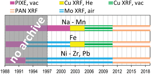
XRF detectors provide raw data in the form of spectra of photon counts versus energy. Elements fluoresce at characteristic energies when inner-shell electrons are dislodged by incident photons of sufficient energy (i.e., X-rays) and the atoms regain stability by filling the vacancies with outer-shell electrons; when the outer-shell, higher-energy electrons drop down to the inner-shell, lower-energy state, they emit photons at energies unique to each element and electron orbital shift. Due to imperfect detection of these X-rays, the spectral lines are broadened into peaks, which sometimes overlap. These peaks must be de-convoluted to quantify the number of photons emitted by individual elements. Next, photon counts are converted to mass loadings through calibrations based on standard reference materials. The CuMo systems employed custom spectral processing software that only integrated portions of the spectra where distinct peaks were identified. In addition, the CuMo system software applied semi-empirical corrections to the mass loadings for particle size and sample loading effects, based on assumptions about particle size distribution and sample composition. The corrections based on particle size applied a constant multiplier to the measured values and were on the order of ~ 10 to 20% of the reported concentrations for Na through Si, dropping to 2% for Ca, and 1% for Fe and S. Loading corrections were applied primarily to adjust for attenuation when fluoresced X-rays are re-absorbed by other particles in the sample matrix and do not reach the detector. The loading corrections were proportional to the sum of measured elemental masses – a minority of the total mass in most samples – and assumed that unmeasured elements (e.g., H, C, O, and N) contributed the same, fixed proportions of every sample’s total mass. While the corrections may have been reasonable approximations for most sites, they were known to overcorrect data at sites with unusual particle composition (White 2017). The E5 instruments process the spectra using non-linear least squares fitting based on Vekemans et al. (1994). The E5 software provides many options for processing the spectra; while the authors chose to apply several corrections for spectral peak overlaps, they did not apply any sample loading or particle size corrections. The E5 systems have several built-in loading corrections available, but the manufacturer advised against using them for thin PM samples. Not applying loading corrections was a significant change coincident with the introduction of the E5 XRF instruments.

The PM_2.5 samples included in this analysis were collected from three IMPROVE sites representing different geographical regions, summarized in Table 1. The Great Smoky Mountains National Park (GRSM1) site is located in the Appalachian Mountains on the eastern United States (US) and presents relatively higher concentrations of sulfur than the other sites. The Point Reyes National Seashore (PORE1) site is located in a marine environment on the California coast, heavily influenced by sea salt. The Mount Rainier National Park (MORA1) site is located at 439 m elevation in the Pacific Northwest region of the US. A total of 1,732 samples were retrieved from the archive and reanalyzed for this study as summarized in Table 1. More information regarding the sample collection and analysis practices in the IMPROVE network can be found in other publications (Hand et al. 2011; Malm et al. 2004) and in the publicly available standard operating procedures (SOPs) hosted online at http://vista.cira.colostate.edu/Improve/sops/ (accessed December 2022).

Table 1. Summary of IMPROVE monitoring locations included in this study.

Site Name	Site Code	Lat/Long	Samples Analyzed	Sampling Date Range
Great Smoky Mountains National Park	GRSM1	35.633 N, 83.942 W	940	June 3, 1995 to November 30, 2009
Point Reyes National Seashore	PORE1	38.122 N, 122.909 W	560	April 3, 2004 to November 30, 2009
Mount Rainier National Park	MORA1	46.758 N, 122.124 W	232	October 24, 2007 to November 30, 2009

All IMPROVE PTFE filter samples collected since March 1995 are archived in a storage building at UCD. Archived samples were stacked in their original slide mounts, wrapped in foil, labeled, and sealed in plastic storage bags. The archive was not refrigerated or rigorously climate-controlled. A previous XRF reanalysis of archived samples showed no elemental degradation with the exception of Br; however, concentration shifts were observed for some elements and were associated with calibrations (Hyslop, Trzepla, and White 2012). The archived filters listed in Table 1 were retrieved and inspected for damage from prior handling and analyses. After retrieval and inspection, the filters from each site were assembled into a queue for analysis on the same instruments used to process 2010 IMPROVE samples: Cu-anode XRF in vacuum for the light elements and Mo-anode XRF in air for the heavier elements. On each instrument, the sample archive for each site was reanalyzed as a continuous batch. Re-inspection revealed new damage after the handling and stress of reanalysis (Hyslop, Trzepla, and White 2015). The stability of the XRF systems was monitored with weekly calibration checks and by analyzing a designated set of filters before and after the reanalysis batches; the results are required to be within 10% of the accepted mean value for each element, except Na and Mg, which are considered qualitative measurements (UCD, 2010). Following these reanalyses in 2012, the CuMo XRF systems were retired. Later, this subset of the archived filters from GRSM1, PORE1, and MORA1 were reanalyzed on the E5 XRF instruments.

Results and discussion

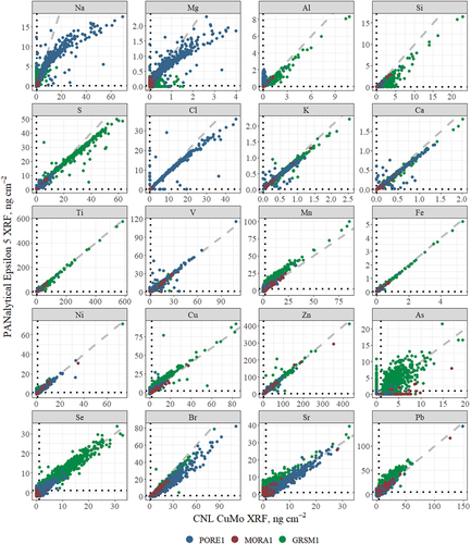
Twenty-four elements are routinely reported for IMPROVE. Figure 2 presents the direct comparison of the measurement results between the two instruments; four elements were excluded (P, Cr, Rb, and Zr) due to low (<50) numbers of pairs above the minimum detection limits (MDL). Clustering around the dashed 1:1 lines is observed for all elements shown, indicating generally good agreement between the two instruments; however, deviations from the 1:1 lines are observed for low Z elements Na, Mg, Al, and Si, as well as the halogens Cl and Br. Na, Mg, S, and Cl agree at lower concentrations, but at higher concentrations, the CuMo system reports higher concentrations than the E5 XRF. The disagreement of the halogens – Cl and Br – may be due to their volatility under vacuum and in storage (Hyslop, Trzepla, and White 2012, 2015). Increased scatter is expected and typical for elements routinely measured near the detection limit, e.g., As (Hyslop, Trzepla, and White 2015). Similarly, trace elements can sometimes be undetectable by the XRF instruments, which report zero. The As panel in Figure 2 shows points along the x = 0 and y = 0 lines, which stand out from the rest of the observations. This was also observed, to a lesser extent, with other elements, e.g., PORE1 Al measurements by the CuMo system.

Figure 2. Scatterplots of the XRF measurements by the two instruments for the twenty elements with at least 50 pairs measured above three times the reported MDLs. The black, dotted lines show the reported MDLs for each element, and the gray dashed lines show 1:1 agreement.

As discussed in the Materials and Methods section, the CuMo systems applied semi-empirical loading corrections to the low Z elements based on the sum of all uncorrected elemental loadings. Figure 3 illuminates the effects of the loading correction by plotting the scaled relative differences (SRD) between the measurements on the two instruments against the sum of all the elements measured on the CuMo systems. SRD is the difference between the two measurements of each element for the same sample normalized by the average of the two measurements, $ScaledRelativeDifference\left(SR{D}_i\right)=\frac{\left(E{5}_i-CuM{o}_i\right)/\sqrt{2}}{\left(E{5}_i+CuM{o}_i\right)/2}$.

Figure 3. Scaled relative differences for Na, Mg, S, and to a lesser extent Cl and K, show strong relationships with the sum of elemental loadings for the CuMo XRF instruments. Al and Si are impacted by another issue, peak overlaps in the Cu-anode detector, which confounds the loading effect.

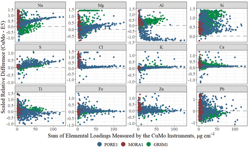
Where E5 is the measurement by the Panalytical E5 instrument, CuMo is the measurement by the CuMo XRF instrument, and i denotes an individual measurement pair. The square root term adjusts for uncertainty in both measurements to provide an estimate of the uncertainty in a single measurement. When only one of the measurements compared is zero, e.g., E5_i = 0 and CuMo_i >0, the SRD (y-axis) value is $-\sqrt{2}$.

In general, individual element mass tends to increase along with the total element mass, and the SRDs are expected to decrease with increasing total element mass, as seen in the Fe and Zn plots. Deviations from that pattern can suggest interferences or artifacts. For some of the light elements, Figure 3 illustrates that the SRDs increase as the sum of the elements increases. These increasing differences, particularly for Na and Mg and less so for S, Cl, K, and Ca, result from the loading corrections. These CuMo system corrections were not appropriate at PORE1, which is a coastal site with high sea salt concentrations, and thus doesn’t fit the typical chemical composition assumed by the corrections. More details regarding this observation and its potential impacts on long-term trends analysis can be found in the publicly available data advisory (White 2017). Al and Si show some different patterns in Figure 3. These two elements were impacted both by the loading corrections and peak interference on the Cu-anode XRF instrument. When S concentrations were high, the shoulder of the S peak on the CuMo system overwhelmed the Al and Si peaks, and these elements were overestimated as seen at GRSM1, an Eastern site that experienced high S concentrations in this time period (Indresand and Dillner 2012). In addition to this documented interference, Al at the PORE1 site is affected by interference from the large Mg peak, causing Al to be reported as zero by the CuMo instrument. Improved detector resolution on the E5 instruments improved these peak overlap issues although some interferences are inevitable at high concentrations. The PORE and GRSM sites were selected for this reanalysis to highlight these issues with the Cu-anode XRF instrument (Indresand and Dillner 2012; White 2006, 2017).

Theil-Sen regression analysis (Sen 1968) was performed on the measurement pairs from the two instruments to quantify agreement. The results for elements with greater than 50 pairs with both measurements greater than or equal to the MDL at the combined three measurement sites are summarized in Table 2. The regression slopes range from 0.34 (Si) to 1.08 (Mn) with most (11 out of 20) having slopes between 0.9 and 1.1. Regression intercepts can be interpreted as an additive bias between the two instruments. Intercepts were statistically significant (p < 0.01) for most elements (except V and Zn) but were small compared to mean concentrations. Relative differences were used to estimate the precision between the two instruments according to (Hyslop and White 2008), as estimated by the standard deviation of the SRD.

Table 2. Number of pairs where each value is greater than or equal to three times the MDL, Theil-Sen regression parameters, precision, and bias for elements with greater than 50 pairs meeting the MDL criterion. The elements P, Cr, Rb, and Zr were excluded by this criterion. Total number of pairs for each element was 1,732. The replicate analytical precision from 2021 and 2022 routine IMPROVE network samples are listed for comparison.

Element	Number of Pairs (> 3 x MDL)	Slope (E5/CuMo)	Intercept (ng cm^−2)	Precision (%)	Bias (%)	Replicate Precision (%)
Na	1236	0.57	499	34	−27	20
Mg	728	0.81	65.8	29	−6	18
Al	1119	0.57	62.7	45	−12	8
Si	1633	0.34	37.1	35	−92	4
S	1729	0.94	84.3	12	−10	2
Cl	482	0.90	−25.4	31	−30	9
K	1729	0.93	13.8	10	−4	2
Ca	1719	0.88	−9.23	14	−22	3
Ti	1405	0.95	0.45	13	−2	9
V	779	0.96	0.01	16	−2	19
Mn	691	1.08	6.49	17	47	11
Fe	1684	0.99	1.56	12	−1	3
Ni	325	0.87	0.41	13	−2	19
Cu	575	1.02	4.09	16	33	11
Zn	1595	1.04	−0.05	11	1	9
As	285	0.59	2.66	25	9	25
Se	912	0.98	0.74	14	5	17
Br	1419	0.78	−1.63	15	−43	14
Sr	686	0.68	2.16	24	10	17
Pb	760	0.99	6.46	17	25	18

(1) $Precision=\sqrt{\frac{1}{N}\sum {\left(SR{D}_i-\overline{SRD}\right)}^{2}X100\mathrm{\%}}$(1)

with N representing the number of measurement pairs included in the calculation. The bias is estimated as the average of the relative differences. Both precision and bias are presented as percentages in Table 2.

(2) $Bias=\frac{1}{N}\sum \frac{\left(E{5}_i-CuM{o}_i\right)}{\left(E{5}_i+CuM{o}_i\right)/2}X100\mathrm{\%}$(2)

For comparison, Table 2 also lists the replicate analytical precision for each element derived from samples collected in 2021 and 2022 and analyzed twice on the E5 instruments. The replicate precision estimates only include contributions from analytical measurement uncertainty on the E5 instrument and provide a threshold value for the comparison between the two instruments (Hyslop and White 2009). Most replicate precisions are lower than the inter-instrument precision values, but curiously a few are higher – V, Ni, Se, and Pb. These higher replicate precision estimates suggest the E5 instrument was less precise than the CuMo instruments for these elements.

Another approach to evaluating the instrument transition is a time-series analysis. Long-term, time-series plots for all 24 measured elements are presented in the Supplemental Information (SI). These plots illustrate the continuity of the measurements across the instrument transition for the bulk of the network. Elements typically measured well above the detection limits show continuous seasonal patterns or otherwise stable network summary statistics across the 2011 transition explored here (e.g., Si, K, and Fe) while other elements show clear steps at the transition (e.g., Na, Cl, Cr, Se, Rb, Sr, and Zr).

An important check on measurement accuracy within the IMPROVE program is inter-species comparisons. Atmospheric sulfur, which is measured by XRF on the PTFE filters, is primarily present in the form of sulfate (Malm et al. 2002; Seinfeld and Pandis 1998), which is concurrently measured by ion chromatography (IC) on the Nylon PM_2.5 filters. Similarly, chloride by IC is comparable to chlorine measured by XRF, although XRF Cl may be biased low relative to chloride because the nylon filters retain chloride more effectively than the PTFE filters (White 2008b). Figure 4 presents the measurements by XRF (3 × S and Cl) with those measured by IC (sulfate and chloride), respectively. In the sulfur-sulfate comparison, the CuMo and E5 measurements are similar. Theil-Sen regression slopes were 1.03 and 0.96 for CuMo and E5, respectively. E5 S measurements are notably low at high S loadings. The E5 and CuMo Cl measurements are biased low compared to chloride, likely related to the filter retention properties. In addition, Cl may volatilize under vacuum during XRF analysis. Therefore, it’s impossible to determine if the differences in the E5 versus CuMo Cl measurements are related to loading corrections applied to the CuMo measurements or volatile losses since the E5 measurements were performed last. In Figure 4c, Na by XRF is compared with chloride (Cl⁻) by IC for both instruments with the dashed line representing the expected molar ratio of Na to Cl⁻ in sea salt. The profile is bifurcated by instrument, owing to the overcorrections by the CuMo systems (blue) and the current underestimations with the E5 instruments (orange) that presumably result from reabsorption of low energy Na fluorescence at high sample loadings.

Figure 4. Comparisons of concurrent measurements for related species reported in IMPROVE. (a,b) compare S and Cl by XRF to sulfate and chloride by IC, respectively. (c) compares Na by XRF to chloride by IC. (d) through (f) compare crustal elements measured by XRF. The gray dashed lines in (a,b) have a slope of one while (c) has a slope of 0.65, the molar ratio of sodium to chloride in NaCl. The gray dashed lines in (d) through (f) represent the bulk continental crust elemental ratios (Taylor and McLennan 1995).

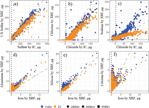
Figures 4d–f present comparisons of lighter crustal elements – Al, Si, and Ca – with Fe. Elements Al and Si were corrected on the CuMo systems and bias estimates are higher than the E5 measurements (Figures 4d,e), whereas Ca had a much lower correction (2%) and bias estimates are more similar between the two instruments. The dashed lines in Figures 4d–f are elemental ratios from the Taylor and McLennan geological survey (Taylor and McLennan, 1995); these are included for reference only and may not be representative of the resuspended dust sampled at the chosen locations. The Al and Si concentrations correlate linearly with Fe while Ca is decoupled from Fe in many samples; indicating independent sources of Ca (e.g., ocean spray).

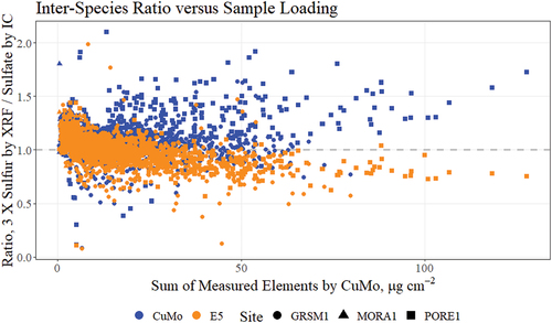
Figure 5 elaborates on the sulfur/sulfate comparison of Figure 4a. The ratio sulfur/sulfate in environmental samples can be greater than $\frac{32\mathrm{A}\mathrm{M}\mathrm{U}}{32\mathrm{A}\mathrm{M}\mathrm{U}+4\times 16\mathrm{A}\mathrm{M}\mathrm{U}}=\frac{1}{3}$, due to non-sulfate sources of sulfur (e.g., organosulfides) as well as differing retention properties between the PTFE and Nylon filters. At heavier loadings, the majority of sulfur mass is empirically found in the form of sulfate aerosols, and the ratio is expected to tend to unity. Heavier sample loadings also tend to experience secondary effects including re-absorbtion of the characteristic X-rays from light elements such as sulfur, resulting in a non-linear response. The loading corrections are proportional to the sum of measured elements from the CuMo instruments. The CuMo 3 X sulfur/sulfate ratio remains > 1 at high sample loadings. The E5 measurements drift below 1 as loadings increase, likely from secondary effects. In Figure 5, the E5 measurements present noticeably less scatter than the CuMo measurements, which indicates greater consistency with the E5 instruments than the CuMo instruments although most of the CuMo S measurement scatter is observed at the PORE site where the matrix correction assumptions were invalid.

Figure 5. Scatterplot highlighting the relationships observed in the sulfur-sulfate ratio with sample loading. The horizontal dashed line represents perfect agreement. The sample loading is estimated using the sum of all elements measured by the CuMo instruments.

Conclusion

A subset of archived IMPROVE samples were reanalyzed on both the legacy CuMo and the present E5 XRF systems. Direct comparisons of the two instruments confirm similar measurement results for most reported elements routinely detected in the network. Low Z elements Na and Mg were overestimated by the CuMo measurements due to systematic corrections for matrix effects based on semi-empirical data. Soil elements Al and Si were affected by spectral interferences on the CuMo instruments. The E5 XRF systems perform well for these elements, which are important for source apportionment analysis. Comparisons of the inter-instrument and E5 intra-instrument precision estimates suggest the E5 instrument measure most elements more precisely than the CuMo instruments, with the exception of V, Ni, Se, and Pb. Multi-year trend analyses that include data prior to the instrument change in 2011 should consider these discrepancies when interpreting results, especially with regard to sea salt (Na, Cl) and crustal (Al, Si) sources. Further inspections of the long-term trends may provide more insight into this instrument transition.

Acknowledgment

The authors thank Warren White for informative discussions and suggestions.

Disclosure statement

No potential conflict of interest was reported by the author(s).

Data availability statement

All IMPROVE data is publicly available through the US EPA Air Quality System (https://www.epa.gov/aqs) as well as through the US Federal Land Manager Environmental Database (http://vista.cira.colostate.edu/Improve/improve-data/). Reanalysis data is available upon request.

Supplementary material

Supplemental data for this paper can be accessed online at https://doi.org/10.1080/10962247.2023.2262417

Additional information

Funding

The work was supported by the United States National Park Service [P11ATW0802].

Notes on contributors

Nicholas J. Spada

Nicholas J. Spada is a scientist in the Air Quality Research Center at the University of California at Davis. Dr. Spada conducts research on elemental profilings in mixed urban/industrial and remote environments. He also provides support on air monitoring strategies and technology to citizen scientists. He is a co-director of the Citizen Air Monitoring Network, based in the Bay Area of California.

Sinan Yatkin

Sinan Yatkin was an Assistant Project Scientist for the Air Quality Research Center at the University of California Davis when this work was performed. He was involved in the research of XRF method development and generation of reference materials.

Jason Giacomo

Jason Giacomo is the Laboratory Operations Manager for the Air Quality Research Center at the University of California Davis. Prior to this role, Dr. Giacomo, was the AQRC Spectroscopist specializing in elemental analysis by X-ray Fluorescence and optical absorption analysis using the AQRC hybrid integrating plate/sphere instrument. Since joining AQRC, Dr. Giacomo has worked to improve the quality control tools available to the lab and to ensure consistent and reliable operation of the analytical instruments in support of atmospheric particulate matter analysis.

Krystyna Trzepla

Krystyna Trzepla was the Laboratory Manager for the Air Quality Research Center at the University of California Davis until her retirement in 2020. Ms. Trzepla provided support for all research studies involving monitoring particles in the atmosphere, with special emphasis on the application of elastic lidar system for monitoring spatial distribution and elemental analyses by X-Ray Fluorescence and Proton Elastic Scattering.

Nicole P. Hyslop

Nicole P. Hyslop is the Associate Director for Quality Research in the Air Quality Research Center at the University of California Davis. Dr. Hyslop conducts research to characterize data quality to gain a better understanding of the sources of error in the measurements and improve quality assurance protocols to identify and reduce errors.

References

- Hand, J.L., S.A. Copeland, D.E. Day, A.M. Dillner, H. Indresand, W.C. Malm, C.E. McDade, et al. 2011. Spatial and seasonal patterns and temporal variability of haze and its constituents in the United States: Report V June 2011. Cooperative Institute for Research in the Atmosphere. http://vista.cira.colostate.edu/Improve/spatial-and-seasonal-patterns-and-temporal-variability-of-haze-and-its-constituents-in-the-united-states-report-v-june-2011/.
- Hyslop, N.P., K. Trzepla, and W.H. White. 2012. Reanalysis of archived improve PM2.5 samples previously analyzed over a 15-year period. Environ. Sci. Technol. 46 (18):10106–13. doi:10.1021/es301823q.
- Hyslop, N.P., K. Trzepla, and W.H. White. 2015. Assessing the suitability of historical PM2.5 element measurements for trend analysis. Environ. Sci. Technol. 49 (15):9247–55. doi:10.1021/acs.est.5b01572.
- Hyslop, N.P., and W.H. White. 2008. An empirical approach to estimating detection limits using collocated data. Environ. Sci. Technol. 42 (14):5235–40. doi:10.1021/es7025196.
- Hyslop, N.P., and W.H. White. 2009. Estimating precision using duplicate measurements. J. Air Waste Manag. Assoc. 59 (September):1032–39. doi:10.3155/1047-3289.59.9.1032.
- Indresand, H., and A.M. Dillner. 2012. Experimental characterization of sulfur interference in improve aluminum and silicon XRF data. Atmos. Environ. 61 (December):140–47. doi:10.1016/j.atmosenv.2012.06.079.
- Malm, W.C., B.A. Schichtel, R.B. Ames, and K.A. Gebhart. 2002. A 10-year spatial and temporal trend of sulfate across the United States. J. Geophys. Res.: Atmos 107 (D22):ACH 11-1–ACH 11–20. doi:10.1029/2002JD002107.
- Malm, W.C., B.A. Schichtel, M.L. Pitchford, L.L. Ashbaugh, and R.A. Eldred. 2004. Spatial and monthly trends in speciated fine particle concentration in the United States. J. Geophys. Res. 109 (D3). doi:10.1029/2003JD003739.
- Murphy, D.M., J.C. Chow, E.M. Leibensperger, W.C. Malm, M. Pitchford, B.A. Schichtel, J.G. Watson, and W.H. White. 2011. Decreases in elemental carbon and fine particle mass in the United States. Atmos. Chem. Phys. 11 (10):4679–86. doi:10.5194/acp-11-4679-2011.
- Seinfeld, J.H., and S. Pandis. 1998. Atmospheric chemistry and physics. New York: John Wiley & Sons.
- Sen, P.K. 1968. Estimates of regression coefficient based on Kendall's tau. J. Am. Stat. Assoc. 63 (324):1379–89. doi:10.1080/01621459.1968.10480934.
- Taylor, S.R., and S.M. McLennan. 1995. The geochemical evolution of the continental crust. Rev. Geophys. 33 (2):241–65. doi:10.1029/95RG00262.
- UC Davis. 2010. Data report for elemental analysis of IMPROVE samples collected during January, February, March 2009. Davis, California: University of California. http://vista.cira.colostate.edu/improve/Data/QA_QC/QAQC_UCD.htm
- Vekemans, B., K. Janssens, L. Vincze, F. Adams, and P. Van Espen. 1994. Analysis of X-ray spectra by iterative least squares (AXIL): New developments. X-Ray Spectr. 23 (6):278–85. doi:10.1002/xrs.1300230609.
- White, W.H. 1997. Deteriorating air or improving measurements? On interpreting concatenate time series. J. Geophys. Res. 102 (D6):6813–21. doi:10.1029/97JD00030.
- White, W.H. 2006. S interference in XRF determination of Si. http://vista.cira.colostate.edu/improve/Data/QA_QC/Advisory/da0011/da0011_S_Si.pdf.
- White, W.H. 2008a. Bias between masked and unmasked elemental measurements. http://vista.cira.colostate.edu/improve/Data/QA_QC/Advisory/da0019/da0019_masks.pdf.
- White, W.H. 2008b. Chemical markers for sea salt in IMPROVE aerosol data. Atmos. Environ. 42 (January):261–74. doi:10.1016/j.atmosenv.2007.09.040.
- White, W.H. 2010. Marginal detection of heavy elements by PIXE analysis. http://vista.cira.colostate.edu/improve/Data/QA_QC/Advisory/da0026/da0026_DA_PIXE_Mo.pdf.
- White, W.H. 2017. Over-reporting of sodium in salt-rich samples. http://vista.cira.colostate.edu/improve/Data/QA_QC/Advisory/da0037/da0037_Na_matrix.pdf.
- White, W.H., L.L. Ashbaugh, N.P. Hyslop, and C.E. McDade. 2005. Estimating measurement uncertainty in an ambient sulfate trend. Atmos. Environ. 39 (36):6857–67. doi:10.1016/j.atmosenv.2005.08.002.
- Yatkin, S., K. Trzepla, W.H. White, N.J. Spada, and N.P. Hyslop. 2020. Development of single-compound reference materials on polytetrafluoroethylene filters for analysis of aerosol samples. Spectrochim. Acta Part B. 171 (September):105948. doi:10.1016/j.sab.2020.105948.