Source characterization of volatile organic compounds at Carlsbad Caverns National Park

ABSTRACT

Carlsbad Caverns National Park (CAVE), located in southeastern New Mexico, experiences elevated ground-level ozone (O₃) exceeding the National Ambient Air Quality Standard (NAAQS) of 70 ppbv. It is situated adjacent to the Permian Basin, one of the largest oil and gas (O&G) producing regions in the US. In 2019, the Carlsbad Caverns Air Quality Study (CarCavAQS) was conducted to examine impacts of different sources on ozone precursors, including nitrogen oxides (NO_x) and volatile organic compounds (VOCs). Here, we use positive matrix factorization (PMF) analysis of speciated VOCs to characterize VOC sources at CAVE during the study. Seven factors were identified. Three factors composed largely of alkanes and aromatics with different lifetimes were attributed to O&G development and production activities. VOCs in these factors were typical of those emitted by O&G operations. Associated residence time analyses (RTA) indicated their contributions increased in the park during periods of transport from the Permian Basin. These O&G factors were the largest contributor to VOC reactivity with hydroxyl radicals (62%). Two PMF factors were rich in photochemically generated secondary VOCs; one factor contained species with shorter atmospheric lifetimes and one with species with longer lifetimes. RTA of the secondary factors suggested impacts of O&G emissions from regions farther upwind, such as Eagle Ford Shale and Barnett Shale formations. The last two factors were attributed to alkenes likely emitted from vehicles or other combustion sources in the Permian Basin and regional background VOCs, respectively.

Implications: Carlsbad Caverns National Park experiences ground-level ozone exceeding the National Ambient Air Quality Standard. Volatile organic compounds are critical precursors to ozone formation. Measurements in the Park identify oil and gas production and development activities as the major contributors to volatile organic compounds. Emissions from the adjacent Permian Basin contributed to increases in primary species that enhanced local ozone formation. Observations of photochemically generated compounds indicate that ozone was also transported from shale formations and basins farther upwind. Therefore, emission reductions of volatile organic compounds from oil and gas activities are important for mitigating elevated O₃ in the region.

Introduction

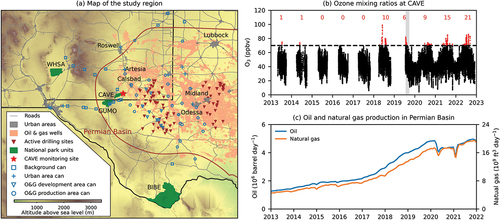
Over the last five years, the frequency of elevated ground-level ozone (O₃) mixing ratios has increased at Carlsbad Cavern National Park (CAVE; Figure 1). High levels of O₃ have detrimental impacts on both human health and vegetation, which is of significant concern in US National Parks (Keiser, Lade, and Rudik 2018; Kohut 2007). Since 2018, the maximum daily 8-hour average (MDA8) O₃ at CAVE (Figure 1b) has regularly exceeded the current National Ambient Air Quality Standard (NAAQS) of 70 ppbv (US NPS 2022). For example, in 2022, there were 21 days with MDA8 O₃$\ge$ 70 ppbv. To address the emerging air quality issues in southeast New Mexico, a series of special studies was conducted to investigate the sources of air pollutants and their precursors, with an emphasis on O₃ formation.

Figure 1. (A) map of the study region, (B) O₃ mixing ratios measured in Carlsbad Cavern National Park (CAVE), and (C) O&G production in the Permian Basin. Grey, pink, and green areas in panel (A) are urban regions, O&G development and production regions (US EIA 2023), and national park units, respectively. Brown line shows the extent of the Permian Basin. Brown triangles show active O&G drilling sites during the 2019 CarCavAQS campaign. Blue squares, crosses, triangles, and circles represent air sampling locations using grab canister samples that reflect air masses in the background, urban, O&G development, and O&G production regions, respectively. See Section 2.1. For how the grab canister samples were categorized. Panel (B) shows O₃ mixing ratios observed at CAVE, and the gray area in panel (B) shows the CarCavAQS period. Red numbers in panel (B) are the number of days with a MDA8 O₃ >70 ppbv. Blue and orange lines in panel (C) show O&G production in the Permian Basin (US EIA 2023).

The formation of tropospheric O₃ occurs when volatile organic compounds (VOCs) are oxidized in the presence of NO_x (NO + NO₂) and sunlight (Chameides et al. 1992). NO_x emissions in the US are dominated by fuel combustion (US EPA 2021). In the western US, however, long-range transport of reservoir species such as peroxyacetyl nitrate (PAN) is also a significant contributor to NO_x (Fischer, Jaffe, and Weatherhead 2011; Lin et al. 2017). VOCs can be emitted from both natural and anthropogenic sources (e.g., (Gu, Guenther, and Faiola 2021)). Natural VOC sources include vegetation (e.g., (Geron et al. 2006; Rasmussen and Went 1965; Zimmerman, Greenberg, and Westberg 1988)), oceans (Fischer et al. 2012), biomass burning (Andreae 2019; Jin et al. 2022), and soil and plant litter (Leff and Fierer 2008). Anthropogenic VOC sources in the US include transportation, oil and gas (O&G) development and production activities, other industrial activities, residential wood burning, and volatile chemical products (Cooper et al. 2012; McDonald et al. 2018; McDuffie et al. 2016; US EPA 2021). Contributions of these emissions to VOC mixing ratios and their capabilities to initiate O₃ production vary significantly across regions (Baker et al. 2008; Benedict et al. 2020). Identifying the relative importance of different sources is critical for designing effective strategies to mitigate elevated O₃ levels at CAVE.

Located in southeastern New Mexico, CAVE is within the Permian Basin and adjacent to Delaware shale play within the Permian Basin. The closest O&G well pad is 6 km to the east. CAVE is sometimes also downwind of the Eagle Ford and Barnett Shale formations located several hundred km to the southeast and east, respectively. The Permian Basin is the most productive O&G regions in the US, and O&G production has increased rapidly from 2013 to 2022 (Figure 1c) (US EIA 2023). Satellite observations show that NO₂ levels are increasing in the region (Dix et al. 2020). Benedict et al. (2020) measured VOC concentrations at four national parks in the southwestern US and found strong influence of anthropogenic sources on VOCs at CAVE and in the surrounding region. This screening study lacked sufficient temporal resolution to capture the full variability of VOCs at CAVE for source characterization and motivated a follow-up study with VOC measurements and NO_x observations at a higher temporal resolution (i.e., hourly).

Here, we present the source characterization of VOCs at CAVE during the Carlsbad Caverns Air Quality Study (CarCavAQS) conducted between July 25^th and September 5^th, 2019. The campaign was designed to investigate the impacts of regional sources on fine particle formation (PM_2.5), VOC composition, O₃ and PAN formation, and nitrogen deposition. The composition, sources, and visibility impacts of PM_2.5 at CAVE have been discussed in Naimie et al. (2022), while O₃, NO_x, and PAN observations are discussed in Pollack et al. (2023). In this work, we characterize sources of VOCs at CAVE using positive matrix factorization (PMF) analysis and consider the contribution of different sources to VOC reactivity.

Method

Monitoring site and VOC sampling

During CarCavAQS, measurements were made at the CAVE Biology Building (32.18°N, 104.44°W; 1355 m above sea level), located within the park and approximately 0.5 km from the visitor center. The major urban center of El Paso-Ciudad Juarez is located 200 km to the west. Smaller cities are located 140 km to the east (Odessa and Midland), 140 km to the north (Roswell) and 30 km to the east (Carlsbad).

Meteorological and O₃ data were collected at the same location by the National Park Service. Mean ambient temperature and relative humidity were 33°C and 36%, respectively, during the campaign. From July to September, the summer monsoon generally transports air masses out from the Permian Basin to the northwest (Figure S1). Therefore, prevailing winds at the site were southeasterly, with occasional gusts from the northwest (Figure S2). When the summer monsoon transport is weak, the site can be more strongly impacted by local and terrain-driven flows, with southeasterly daytime upslope flows and nocturnal northeasterly downslope flows (Crosman 2021). During the summer of 2019, the site was impacted by a subtropical ridge over southern New Mexico, which suppressed the monsoon transport out of the Permian Basin to the west (Figure S1) and led to more frequent northwesterly winds at CAVE (Figure S2). To qualitatively distinguish the origins of air masses, observations are grouped into south-to-southeast (S-SE) and north-to-northwest (N-NW) wind sectors (Figure S1). The S-SE wind sector, the direction of the Permian Basin, ranges from 90° to 225°, with 0° representing north and 180° representing south. Wind directions larger than 270° or less than 45° are within the N-NW wind sector, and air masses from this sector typically represent background conditions.

To investigate VOC composition near and away from sources, 66 air samples were also collected at various locations using grab canister samples. Stainless steel Silonite®-coated 1.4 L canister samples (Entech Instruments) were used. A comprehensive description of canister cleaning and sampling procedures is available in Benedict et al. (2020). Sampling locations were selected to reflect background conditions (blue squares in Figure 1) and air masses impacted by urban/traffic emissions (blue crosses), O&G development activities (blue triangles), and O&G production activities (blue circles). Grab canister samples collected within 10 km of an O&G site being developed during CarCavAQS, were considered influenced by O&G development (n = 10). Samples were deemed impacted by O&G activities if they were collected within 10 km of an O&G producing well pad and were not in urban areas or heavily impacted by traffic (n = 25). Note that for some locations it is challenging to distinguish impacts from urban and O&G emissions.

Measurements

Measurements discussed in this work include O₃, methane (CH₄), NO_x, total reactive nitrogen (NO_y), PAN, and non-methane VOCs (NMVOCs). Detailed descriptions of each measurement can be found in Text S1 of the supporting information (SI). Briefly, O₃ was measured by a Thermo 49i O₃ analyzer. CH₄ was measured via cavity ringdown absorption spectroscopy (Picarro, G2508). NO, NO₂, and NO_y were measured using a single-channel commercial NO analyzer (Eco Physics, model CLD 780 TR) employing NO-O₃ chemiluminescence detection and outfitted with two custom-built inlets (Pollack, Lerner, and Ryerson 2010). PAN was measured using a custom-built gas chromatograph (GC) instrument using a commercial electron capture detector.

A five-channel, three-GC analytical system was used to analyze 56 individual VOCs in real-time (hourly time resolution), including light alkanes (C₂-C₇), heavy alkanes (C₈-C₁₀), C₁-C₂ halocarbons, C₁-C₅ alkyl nitrates, alkenes, branched alkanes, branched alkenes, cyclic alkanes, aromatic VOCs, and biogenic VOCs (Abeleira et al. 2017). A similar lab-based system was also used to analyze VOCs in the grab canister samples (Benedict et al. 2020). In addition to the GC system, a proton transfer reaction-mass spectrometer (PTR-MS; PTR-MS HS, Ionicon Analytik) was deployed to measure acetonitrile, isoprene, and select oxygenated VOCs (OVOCs), including acetone, methyl ethyl ketone (MEK), and methyl vinyl ketone (MVK). A complete list of VOCs measured and corresponding measurement precisions and method detection limits (MDLs) are provided in Table S1.

The inlets of these instruments were positioned approximately 6–7 m above the ground. All measurements were averaged to one hour to synchronize the data, although instrument sampling frequencies ranged from one minute to one hour.

Positive matrix factorization

PMF has been widely used as a source apportionment technique for VOCs (Abeleira et al. 2017; Bon et al. 2011; Brown, Frankel, and Hafner 2007; Pollack et al. 2021; Ulbrich et al. 2009; Yuan et al. 2012). PMF is a receptor model that decomposes a matrix of speciated sample data ($X$) into factor profiles ($F$) and their contributions ($G$):

(1) $\begin{array}{c}X=G\cdot F+E.\end{array}$(1)

The sample data matrix ($X$) has a dimension of $m\times n$, where $m$ is the number of species and $n$ is the number of samples. The factor profile matrix ($F$) has $p\times m$ elements, which are often interpreted as fingerprints of VOC sources or the stages of photochemical processing (Yuan et al. 2012) and are assumed to be constant over the duration of the campaign. Factor contributions vary and reflect the relative importance of different sources. The factor contribution matrix (G) has $n\times p$ elements, representing the contributions of the factors. The residual matrix ($E$) represents data points not fully fit by the model.

The EPA PMF Model (v5.0) is used in this study, which solves Equation (1)(1) $\begin{array}{c}X=G\cdot F+E.\end{array}$(1) using the constraint that no sample can have significantly negative source contributions (Paatero 1997, 1999). The tool uses both sample concentrations and measurement uncertainties to weight individual data points when calculating and minimizing the objective function $Q$. Samples and uncertainties used in our PMF analysis were prepared following Hopke (2016) and Polissar et al. (1998). VOC measurements with mixing ratios above the corresponding MDL were used directly as inputs and assigned uncertainties listed in Table S1. However, some VOC species had unclear or indiscernible chromatogram peaks for certain periods and were deemed below their MDLs. In this case, the corresponding MDLs divided by three were used as inputs, and 5/6 times the MDLs were assigned as uncertainties. Weighting data points this way allows the level of confidence in the measurement to be accounted for in the PMF model solution. In addition, signal-to-noise ratios (S/N) were considered before running the PMF model. Following Hopke (2016), 11 VOC species with S/N < 0.5 were flagged as “bad” and excluded from the PMF analysis. In total, 47 species and 573 samples from the real-time GC and PTR-MS data were included in the PMF analysis.

Determining the number of factors used in the PMF model is important so that the solution can represent source characterization appropriately. A sufficient number of factors is required to explain the variability in the dataset. However, when too many factors are included, physically relevant factors can be separated into multiple unrealistic factors, known as “factor splitting” (Brown, Frankel, and Hafner 2007; Ulbrich et al. 2009). In this work, PMF solutions with numbers of factor ranging from 3 to 9 were evaluated, and the solution with seven factors was selected because it significantly reduces the model error without unreasonable splitting of factors. Details for selecting the seven-factor PMF solution are provided in Text S2 and Figure S3–S7.

We estimated the uncertainties of factor profiles and contributions from 100 bootstrapping runs (Ulbrich et al. 2009). Figures and tables throughout this work show factor profiles and factor contributions from the PMF solution, and uncertainties represent the mean and the 25^th and 75^th percentiles from the 100 bootstraps. We note that the mean and median values determined from bootstrapping are nearly identical in the PMF solution (Figure 2). We also found that no additional matrix rotation or constraints were needed to optimize the solution (Figure S8) (Paatero and Hopke 2009).

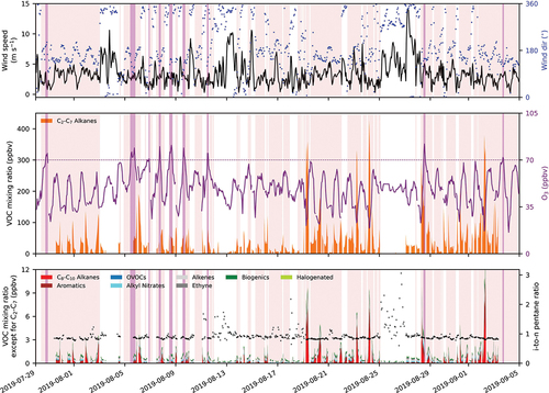
Figure 2. Meteorological conditions, O₃ mixing ratios, and NMVOC mixing ratios at CAVE during the CarCavAQS. The top panel shows wind speed (black) and wind direction (wind dir; blue) observations. The filled areas and the purple line in the bottom panel show VOC and O₃ mixing ratios measured at CAVE. The bottom panel shows the VOC mixing ratios for species other than the C₃-C₇ alkanes. The pink- and purple-shaded areas show periods with southerly and southeasterly winds and high O₃ (70 ppbv), respectively.

HYSPLIT backward trajectories and residence time analysis

Backward trajectories were calculated using the Hybrid Single Particle Lagrangian Integrated Trajectory (HYSPLIT) model (Stein et al. 2015). A detailed description of the model setup is provided in Naimie et al. (2022). HYSPLIT trajectories and source-receptor relationships were investigated using residence time analysis (RTA) (Gebhart et al. 2018, 2021). The residence time is the amount of time an air mass spends in a horizontal grid cell (0.25° × 0.25°), which is represented by the everyday probability (EP). High-concentration residence time or high probabilities (HP) are calculated using trajectories from the top 10% concentration values at the receptor site. These two residence times can be compared using the incremental probability (IP = HP – EP) to determine if the probability of an endpoint being in a grid cell is more likely during the high concentration periods or throughout the dataset.

VOC-OH reactivity

The potential of a VOC species to initiate the O₃ formation cycle is partly driven by its reactivity with the OH-radical, $R_{\mathrm{O}\mathrm{H},\mathrm{V}\mathrm{O}\mathrm{C}}$ (s⁻¹) $R_{\mathrm{O}\mathrm{H},\mathrm{X}}$ is calculated as the inverse of the lifetime of OH reaction with species X as:

(2) $\begin{array}{c}{R}_{\mathrm{O}\mathrm{H},\mathrm{X}}=k_{\mathrm{O}\mathrm{H},\mathrm{X}}\left[\mathrm{X}\right],\end{array}$(2)

where $k_{\mathrm{O}\mathrm{H},\mathrm{X}}$ is the rate constant at 298 K (obtained from Atkinson and Arey (2003) and Atkinson (1986)) and $\left[\mathrm{X}\right]$ is the number density of X in molecule cm⁻³. Although this simplified estimate does not consider reactions with other oxidants, nor does it consider chain propagation or termination steps resulting from reaction with OH, $R_{\mathrm{O}\mathrm{H},\mathrm{V}\mathrm{O}\mathrm{C}}$ has been widely used to provide valuable insights into the potential for a VOC to contribute to O₃ production, as the initial reaction with OH is often the limiting step in the sequence of reactions to form O₃ (Abeleira et al. 2017; Benedict et al. 2020; Gilman et al. 2013; McDuffie et al. 2016; Rutter et al. 2015).

Photochemical aging

To understand the sources of secondary VOCs and their relationships with O₃ formation, we also estimated photochemical air mass ages using ratios of concentrations of two alkyl nitrates to their corresponding parent hydrocarbons (RONO₂/RH). Alkyl nitrates are formed when n-alkanes are oxidized (Simpson et al. 2003). Therefore, the ratio of a daughter alkyl nitrate to its parent n-alkane increases as an air mass ages (Benedict et al. 2020; Bertman et al. 1995; Russo et al. 2010; Simpson et al. 2003). We use 2-pentyl nitrate/n-pentane and 2-butyl nitrate/n-butane ratios to construct a photochemical clock based on measured and modeled ratios. The modeled ratios are calculated using laboratory kinetic data (Bertman et al. 1995), assuming $\left[\mathrm{O}\mathrm{H}\right]={10}^6$ molecules cm⁻³ and that OH-initiated photochemical production is the only source of the given alkyl nitrates. Since the estimated photochemical ages using this method scale with [OH], they are only approximate, allowing for comparing relative photochemical processing among different air masses. In addition, deviations from the modeled relationship are expected because additional sources and sinks are not considered. More details of the model are provided in Text S3.

Results

VOC observations and VOC OH reactivities

Figure 2 shows meteorological conditions, O₃ mixing ratios, and NMVOC mixing ratios at CAVE during CarCavAQS. C₂–C₇ alkanes (orange areas in Figure 2) dominated NMVOCs during the campaign, and time series of other species are provided in the bottom panel of Figure 2. Mean VOC concentrations and $R_{\mathrm{O}\mathrm{H},\mathrm{V}\mathrm{O}\mathrm{C}}$ at CAVE for the whole campaign and periods with different wind directions are shown in Figure 3. The contribution of OVOCs to VOC OH reactivity might be underestimated since only a few OVOCs were measured (i.e., acetone, MEK, and MVK). Figure 3 also shows the mean VOC concentrations and $R_{\mathrm{O}\mathrm{H},\mathrm{V}\mathrm{O}\mathrm{C}}$ in canister samples collected in different regions. We note that OVOCs and acetonitrile were not analyzed in the canister samples.

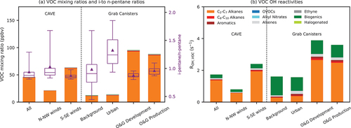
Figure 3. (A) Mean VOC mixing ratios, i-to n-pentane ratios, and (B) mean OH reactivities observed at CAVE under different winds and in the grab canister samples. The boxes and whiskers in panel (A) show the 5^th, 25^th, 50^th, 75^th, and 95^th percentiles of the i-to n-pentane ratios. The triangles in panel (A) show the mean i-to n-pentane ratios. Note that acetonitrile and OVOCs, including acetone, MEK, and MVK, were not measured in the canister samples.

Observations made at CAVE are categorized into S-SE and N-NW wind sectors as defined in Section 2.1 and accounted for 59% and 33% of the time with valid observations. High total VOC episodes (>100 ppbv) occurred mostly with wind from the S-SE wind sector except for one event on 08/19 during which the locally observed wind direction shifted between the two wind sectors. Short-term wind direction shifts occurred mostly as a part of the wind diel pattern. VOC mixing ratios remained low when CAVE experienced consistent N-NW winds (e.g., 08/25–08/27). High O₃ (purple-shaded areas in Figure 2) only occurred when winds were from the S-SE wind sector (pink-shaded areas in Figure 2) but did not always align with high VOC periods.

To better illustrate VOC composition, VOCs are grouped into nine categories: light (C₂-C₇) alkanes, heavy (C₈-C₁₀) alkanes, aromatics, OVOCs, alkyl nitrates, alkenes, ethyne, biogenics, and halogenated compounds. Tables S1 and S2 list compounds in each group and summary statics for concentrations at CAVE and in grab canister samples. Consistent with Benedict et al. (2020), light alkanes dominated VOCs observed at CAVE and in the grab canister samples collected in the area. Although certain light alkanes can be emitted from combustion sources, light alkanes are generally considered good markers for O&G sources (Abeleira et al. 2017; Benedict et al. 2020; Gilman et al. 2013; Swarthout et al. 2013). VOC mixing ratios during periods with N-NW winds were slightly higher than those in the canister samples from background and urban regions. The background and urban canister samples also had higher biogenic but lower light alkanes. The difference in VOC mixing ratios and compositions indicate that locally measured winds may not fully represent regional transport patterns, especially when the diel wind pattern was dominated by terrain-driven flows. Thus, further analyses of canister samples and backward trajectories are needed to better link VOCs observed at CAVE to sources.

The i-to n-pentane ratio can be used to distinguish emissions between O&G or combustion emissions. An i-to n-pentane ratio much larger than one implies strong influence from combustion sources, including vehicular emissions (Russo et al. 2010b), while a ratio less than one indicates substantial influence from O&G emissions (Evanoski-Cole et al. 2017; Gilman et al. 2013; Swarthout et al. 2013). Measured i-to n-pentane ratios at CAVE ranged between 0.8 and 1.5, and values below one were observed mostly during periods with S-SE winds (Figures 1 and 3). The pattern of i-to n-pentane ratios observed at CAVE is consistent with patterns observed in grab canister samples collected in background areas and urban regions showed higher i-to n-pentane ratios with larger variability compared to those collected in O&G development and production regions. This consistency suggests that wind directions can be used to distinguish air masses impacted by O&G activities and other sources.

At CAVE, light alkanes also dominated VOC OH reactivities. Air masses from the S-SE wind sector passing through the Permian Basin had higher total OH reactivity for measured VOCs, indicating strong influence of O&G emissions. Although reactive OVOCs and acetonitrile were not measured in the grab canister samples, grab canister samples collected in O&G development areas showed the highest total OH reactivity, which corroborates the importance of O&G emissions for O₃ formation. Concentrations of biogenic compounds were low, but they were still the second most important contributor to OH reactivity at CAVE because they are highly reactive with OH. In the canister samples collected in background and urban areas, biogenics were the main contributor to total OH reactivity despite being a desert environment. Alkenes were typically the third contributor to OH reactivity at CAVE, followed by OVOCs and heavy alkanes.

The wind direction, tracer ratio, and grab canister sample analyses identify the differences in VOC composition and VOC OH reactivities of different sources. However, they do not explain why O₃ increases were associated with both high total VOC (08/28) and substantially lower total VOC (08/05–09, and 08/11). A PMF analysis could help illustrate the differences between these cases.

PMF factors

Using the NMVOC observations from the on-line five-channel GC system and the PTR-MS at CAVE, the PMF model identified seven factors, which were labeled as follows: (1) longer-lived O&G, (2) shorter-lived O&G, (3) process-specific O&G, (4) longer-lived secondary, (5) shorter-lived secondary, (6) alkenes, and (7) background. Figure 4 shows factor contributions to each VOC species considered in the PMF analysis, and Figure 5 shows their diel and wind direction profiles. NO_x, O₃, and PAN were left out of the PMF analysis to be used as tracers to facilitate the characterization of the PMF output, and their diel profiles are also presented in Figure 5. Time series of the contributions of the PMF factors are shown in Figure S10, and reconstructed time series of selected compounds from different groups using the PMF factors are shown in Figure S11.

Figure 4. PMF factor profiles. The bars represent the contribution of the factor to each species, and error bars represent the 25^th and 75^th percentiles of the contributions from the 100 bootstrapping runs. Dots show the mean values of the bootstrapping runs.

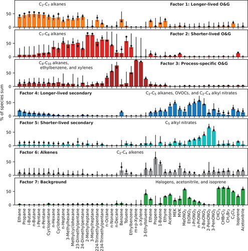
Figure 5. Diel and wind direction profiles of factor contributions. Colored triangles and lines in panels (A–C) show 2-hr means of factor contributions. Boxes and whiskers in panels (A–C) are the 5^th, 25^th, 75^th, and 95^th percentiles of the 2-hr composite distributions of the factors. Diel patterns (2-hr means) of NO, NO_y, O₃, PAN (multiplied by 200), wind direction (WD), and solar radiation (SR) are also shown in panels (A–C). Panel (D) shows 30°-wind-direction means of factor contributions.

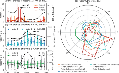
Factors 1, 2 and 3 are consistent with emissions from O&G activities. The longer-lived O&G factor (factor 1) accounts for 20–50% of the observed C₂–C₇ alkanes and is consistent with contributions of O&G factors to these alkanes reported in previous studies in other O&G-producing regions (Abeleira et al. 2017; Gilman et al. 2013; Pollack et al. 2021; Swarthout et al. 2015). The C₇ alkanes, especially branched ones, contribute significantly to the shorter-lived O&G factor (factor 2), along with C₈ alkanes. Emissions of these alkanes have been closely linked to specific activities associated with O&G extractions, such as flashing from oil and condensation tanks (Warneke et al. 2014). The process-specific O&G factor (factor 3) is dominated by C₉–C₁₀ alkanes, ethylbenzene, and xylenes. High emissions of these species have been observed during O&G development processes, such as drilling, fracking, and flowback (Hecobian et al. 2019). In studies in the Denver-Julesburg (DJ) Basin, elevated emissions of C₈-C₁₀ alkanes have been reported specifically during well-drilling operations (Lachenmayer 2022). All three factors are associated with S-SE winds from the Permian Basin. Thus, the diel patterns of contributions of these factors are similar. Their contributions decreased in the afternoon, indicative of dilution resulting from boundary layer deepening. Contributions of these three factors correlate well with each other (R² ranging from 0.37 to 0.76; Figure S9) and with CH₄ (Figure S12). The correlation between the process-specific O&G factor and CH₄ is lower than for the other two O&G factors; this is not surprising given that CH₄ emissions can vary significantly relative to VOC emissions across well development activities.

Secondary VOC species (e.g., OVOCs and alkyl nitrates) produced by photochemical reactions map into two factors. Both factors have an i-to n-pentane ratio lower than one, suggesting their O&G origins. A longer-lived secondary factor (factor 4) is dominated by OVOCs and C₁-C₄ alkyl nitrates. Yuan et al. (2013) showed that longer-lived species like C₃-C₅ alkanes can be a principal source of acetone in some environments. Thus, we postulate that the C₁-C₄ alkyl nitrates and OVOCs associated with the longer-lived secondary factor arise from similar photochemical reactions of light alkanes associated with the longer-lived O&G factor. This hypothesis is supported by the fact that the longer-lived secondary factor always consists of both a fraction of light alkanes and C₁-C₄ alkyl nitrates regardless of the number of factors (Figure 4 and S4–S7). The shorter-lived secondary factor is enriched in larger (e.g., C₄ and C₅) alkyl nitrates, which have shorter lifetimes than smaller alkyl nitrates (Bertman et al. 1995). Diel patterns of the two secondary factors have a pronounced daytime rise. However, the shorter-lived secondary factor has a similar diel pattern to those of PAN and solar radiation, whereas the longer-lived secondary factor peaks later in the afternoon, suggesting they were likely aged air transported from farther upwind and entrained from above the mixed layer. The shorter-lived secondary factor is largely associated with S-SE winds, while the longer-lived secondary factor is largely correlated with easterly winds.

The sixth factor is dominated by light alkenes and the seventh factor is mostly comprised of isoprene, halogenated compounds, and acetonitrile. Unlike the O&G and secondary factors, the alkene factor has a mean i-to n-pentane ratio larger than one (1.2), suggesting stronger influence on this factor from combustion sources. Light alkenes have been linked to vehicular emissions in urban areas and O&G production regions (Baker et al. 2008; Swarthout et al. 2013) but also can be emitted by industrial activities (Washenfelder et al. 2010), vegetation (Rhew et al. 2017), and biomass burning (Akagi et al. 2012; Hecobian et al. 2011). CAVE was not significantly impacted by wildfire plumes in 2019 during CarCavAQS (Pollack et al. 2023). Since CAVE is more than 140 km away from major urban centers and high contributions of the alkene factor occurred mostly with S-SE winds, we hypothesize that the alkene factor may reflect influence from vehicular or other combustion emissions associated with O&G activities in the Permian Basin. However, vehicular emissions from the Facilities area near the site could also contribute to the alkene factor. The seventh factor is comprised of species with long lifetime or natural sources and shows little correlation with other trace gases (Figure S9) and weak wind direction dependence. This factor is interpreted as representing the regional background.

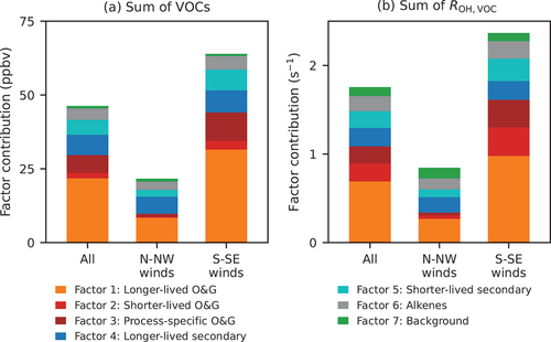
On average, the long-lived O&G factor had the largest contribution to observed VOCs and their OH reactivities at CAVE during CarCavAQS (Figure 6), followed by the process-specific O&G factor. During periods with S-SE winds, contributions of the three O&G factors increased. The two secondary factors also contributed significantly to the measured VOCs, especially during periods when O₃ was high, whereas contributions of the three O&G factors decreased during high O₃ events compared to other periods with S-SE winds, especially the process-specific O&G factor 3 (Pollack et al. 2023).

Figure 6. Mean factor contributions to measured VOCs at CAVE during summer 2019 their OH reactivities for the whole duration of CarCavAQS and periods with southerly and southeasterly (S-SE) winds, and northerly and northwesterly (N-NW) winds.

Linking PMF factors to sources

Although the wind direction analyses shown above roughly point to the source regions of different VOC species and PMF factors, in-situ wind measurements near the surface at CAVE may be impacted by local terrain effects and not correctly represent regional transport patterns. In addition, confirmation is needed for the attribution of the PMF factors based mostly on previously reported tracers observed near different sources, especially for the process-specific O&G factor. Emission profiles for these processes in the Permian Basin might be different from those reported for the DJ Basin. Therefore, we further applied the PMF results to grab canister observations and conducted RTAs to better link VOC observations and PMF factors to different source regions.

To check if the PMF analysis correctly captured the characteristics of different sources in the regions, we solved Equation (1)(1) $\begin{array}{c}X=G\cdot F+E.\end{array}$(1) for all grab canister samples using a non-negative least squares solver with the factor matrix from our PMF analysis based on CAVE observations (Lawson and Hanson 1987). More details are provided in Text S4. Note that acetonitrile and OVOCs, including acetone, MEK, and MVK, were not measured in the canister samples and were removed from the fitting. The estimated contributions are normalized using all canister means to show the relative importance of a factor from different sources, and mean normalized contributions are shown in Figure 7. The highest contributions of the shorter-lived O&G, process-specific O&G, and shorter-lived secondary factors were observed near active drilling sites. Samples from O&G production regions showed the highest contribution of the longer-lived O&G factor. The alkene factors were observed in urban/traffic, O&G development, and O&G production canister samples. The background factor was relatively consistent near different sources. Thus, PMF contributions derived from source-dominated air samples are generally consistent with our attribution, providing additional support to the PMF analysis.

Figure 7. Mean normalized contributions of the PMF factors to air sampled in different areas. The factors are the same as the ones shown in Figure 4 but without acetone, MEK, and MVK. The contributions are normalized using all canister means to show the relative importance of a factor in different areas. The black bars show the mean normalized residuals of the fittings.

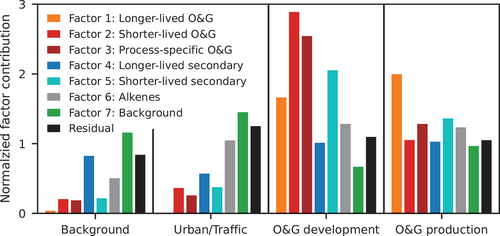
VOCs sampled in grab canister samples collected near O&G development and production sites show large variability and relatively large residuals when fitted with the PMF factors (see Table S3 and Figure S13). The samples strongly influenced by local sources actually have larger fitting errors (Figure S13), indicating that the PMF factors derived from CAVE observations represent aged air masses. The large variability likely arises from the challenges associated with obtaining representative samples for these sources in close proximity because the wind direction and atmospheric conditions could be non-ideal while emissions and plume interception can both be intermittent. Therefore, instead of using the VOC observations from air samples to conduct source attribution with the PMF method or a chemical mass balance approach directly, we only used the canister results as a check on factor assignments in our PMF analysis.

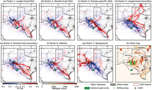
In addition to applying the PMF results to the grab canister observations, we also conducted RTA to investigate the transport pathways associated with different factors. Figure 8 shows the IP distributions using 48-hour backward trajectories for the seven PMF factors. Air masses with a high contribution (top 10%) of a factor were more likely to have passed through the red grid cells than the blue cells. High contribution periods of the three O&G factors (Figure 8a-c) and the alkene factor (Figure 8f) had a similar transport pattern, predominantly passing through O&G development and production areas in the Permian Basin and Eagle Ford Shale formation to the southeast of CAVE. The high contribution of the shorter-lived secondary factor was associated with transport from the southeast and the east sectors (Figure 8e). However, trajectories through central, north, and northwest Texas, Oklahoma, and Kansas contributed more to periods with high contribution of the longer-lived secondary factor (Figure 8d). These air masses might have been impacted by multiple sources at different times, including urban and industrial emissions as well as O&G emissions in the Permian Basin, the Eagle Ford Shale, the Barnett Basin Shale, or the Anadarko Basin in Oklahoma. High contributions of the background factor were associated with transport from the west (Figure 8g).

Figure 8. Incremental probability maps of the PMF factors from the RTA (A–G) and a map of potential sources (H). The IPs are based on 48-hour back trajectories and are distance normalized by multiplying each grid cell value by the distance from the origin site (yellow star). The grid cell resolution is 0.25 degrees square. Grids in panel (H) are colored by the number of O&G well pads in the cell (US EIA 2023). Grey lines and areas show major highways and urban areas, respectively. Brown lines show major boundaries of the O&G basins and shale formation. Green areas show national park units. Green crosses in panel (H) show locations of active drilling sites during CarCavAQS.

Photochemical aging

Figure 9 shows 2-pentyl nitrate-to n-pentane ratios versus 2-butyl nitrate-to n-butane ratios derived from the observations at CAVE and grab canister samples as well as the relationship between the two ratios modeled based on laboratory parameters (Bertman et al. 1995). The relationship between the two ratios can be used as a photochemical clock to infer the photochemical aging of air masses (Benedict et al. 2020). The modeled photochemistry matched the values derived from canister samples collected near O&G development and production sources. Canister samples with a shorter photochemical age often had a higher ethane (C₂H₆) mixing ratio, a good indicator for O&G emissions (Benedict et al. 2020, Evanoski-Cole et al. 2017; Swarthout et al. 2013, 2015). The good agreement between the modeled and observed ratios provides support for using the photochemical clock for air masses strongly influenced by O&G emissions, whose alkyl nitrates are mostly generated through OH-initiated reactions. For the canister samples representing background and urban conditions, there were larger discrepancies between the modeled and observed ratios, suggesting factors not included in the model played a more important role, such as other possible sources and removal mechanisms for 2-pentyl and 2-butyl nitrates, and varying branching ratios (Benedict et al. 2020).

Figure 9. Photochemical clocks using ratios of 2-pentyl nitrate (2-PenONO₂)/n-pentane and 2-butyl nitrate (2-BuONO₂)/n-butane for (A) grab canister air samples, (B–D) all observations at CAVE with data points colored by C₂H₆, PAN, and O₃ mixing ratios. The lines represent the modeled data. Colored squares, crosses, triangles, and dots in panel (A) represent ratios derived from grab canister samples collected near background, urban/traffic, O&G development, and O&G production areas, respectively.

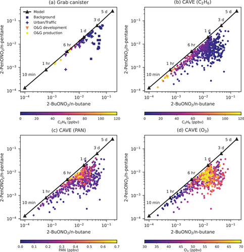
The photochemical clock suggests that air masses observed at CAVE might have undergone two different modes of photochemical processing. Fresh air masses generally had a high C₂H₆ mixing ratio, consistent with results for grab canister samples, and low PAN and O₃ mixing ratios. For aged air masses (>6 hours), there were two clusters. One cluster matched the calculated ratios, and PAN and O₃ mixing ratios increased as they went through photochemical aging. Air masses in the other cluster deviated from the calculated ratios. Despite having similar O₃ mixing ratios, their C₂H₆ and PAN levels were much lower than those of air masses in the first cluster, suggesting longer photochemical ages than the ones predicted by the photochemical clock. The discrepancies could result from varying OH concentrations and/or photolysis rates during the history of the air mass (Benedict et al. 2020).

Conclusion and implications

During CarCavAQS, C₂-C₇ alkanes dominated both observed VOC mixing ratios (98% on average) and VOC OH reactivities (79% on average), consistent with the findings from Benedict et al. (2020). These alkanes were generally associated with air masses from the S-SE and with i-to n-pentane ratios < 1. These air masses had a similar VOC composition in the grab canister samples collected near O&G development and production sites. Three of the PMF factors were attributed to O&G activities, comprising VOC profiles previously reported for O&G production and development activities. Contributions of these factors were significantly higher during periods with S-SE winds (69% to VOC mixing ratios) than periods with N-NW winds (45% to VOC mixing ratios). Our RTA further confirmed that the O&G factors were associated mainly with transport from the south and southeast, an area of significant O&G development and production activities.

Our PMF analysis also identified two secondary factors with different atmospheric lifetimes, suggesting that air masses observed at CAVE might have different photochemical ages. Both factors are likely oxidation products of O&G emissions as indicated by their i-to n-pentane ratios less than one. The contribution of the shorter-lived secondary factor was higher from the S-SE based on our wind direction analysis and the RTA. Its contribution typically peaked around noon (10:00–14:00) with the highest solar radiation. Therefore, the air masses with an increased contribution of shorter-lived secondary factor might have been transported during the day directly from source regions near CAVE (e.g., Permian Basin) with freshly produced secondary species. Similar diel patterns have been observed in Northern Colorado in summer 2015 (Abeleira et al. 2018). The diel pattern of the longer-lived factor peaked later in the afternoon (14:00–18:00), which could be related to boundary layer development and entrainment. O₃ increases were observed during periods with high contributions of both shorter-lived and longer-lived factors, and the O₃ diel pattern had a broad peak (10:00–18:00). The RTA showed that air masses with a high contribution of longer-lived secondary factor might have been transported from source regions further upwind from the southeast, the east, and the northeast. The longer-lived secondary factor also consisted of less reactive light alkanes but lacked more reactive heavy alkanes, suggesting the longer-lived secondary species were photochemical products of VOC and NO_x emissions from O&G activities.

Our photochemical clock model shows that O₃ enhancements were related to both locally and regionally formed O₃. A fraction of the air masses with both high O₃ and PAN mixing ratios had a photochemical age between 6 to 12 hours, showing the impacts of locally formed O₃. However, a fraction of high O₃ plumes had a photochemical age longer than the daytime duration (12 hours). For these plumes, the transport time might be significantly longer than the photochemical age since the [OH] of 10⁶ molecules cm⁻³ used in the photochemical clock model represents daytime conditions with high photolysis rates and nighttime [OH] is usually one or two orders of magnitude lower (Bey, Aumont, and Toupance 1997). Therefore, these plumes may reflect air masses stagnated near CAVE overnight or sources located more than one day upwind of CAVE.

The source apportionment shown here establishes the dominant influence of O&G activities on both primary and secondary VOC at CAVE, which likely affects local and regional O₃ formation. A more comprehensive modeling effort is needed to investigate local and regional photochemistry and their impacts on elevated O₃ at CAVE and in the region, including Carlsbad, NM which has also been experiencing O₃ exceedance.

Acknowledgments

We thank the Carlsbad Caverns National Park staff and scientists for their support with project logistics.

Disclosure statement

No potential conflict of interest was reported by the author(s).

Data availability statement

The data from the 2019 CarCavAQS that support the findings of this study are openly available in https://doi.org/10.25675/10217/235481

Supplementary material

Supplemental data for this paper can be accessed online at https://doi.org/10.1080/10962247.2023.2266696

Correction Statement

This article has been corrected with minor changes. These changes do not impact the academic content of the article.

Additional information

Funding

This work was supported by the National Park Service under Agreement Number P20AC00679 with Colorado State University.

Notes on contributors

Da Pan

Da Pan is a Research Scientist I in Atmospheric Science at Colorado State University.

Ilana B. Pollack

Ilana B. Pollack is a Research Scientist III in Atmospheric Science at Colorado State University.

Barkley C. Sive

Barkley C. Sive is an atmospheric chemist in the Air Resources Division of the National Park Service. Dr. Sive serves as the Program Manager for the Gaseous Pollutant Monitoring Program (GPMP).

Andrey Marsavin

Andrey Marsavin is a Ph.D. student at Colorado State University in Atmospheric Science.

Lillian E. Naimie

Lillian E. Naimie is a Ph.D. student at Colorado State University in Atmospheric Science.

Katherine B. Benedict

Katherine B. Benedict is a Research Scientist at Los Alamos National Laboratory. Dr. Benedict was a Research Scientist in Atmospheric Science at Colorado State University during the 2019 field study.

Yong Zhou

Yong Zhou is a Research Scientist II in Atmospheric Science at Colorado State University.

Amy P. Sullivan

Amy P. Sullivan is a Research Scientist III in Atmospheric Science at Colorado State University.

Anthony J. Prenni

Anthony J. Prenni is a Chemist in the Air Resources Division of the National Park Service.

Elana J. Cope

Elana J. Cope is a Ph.D. student at the University of Oregon in Chemistry, and was an undergraduate student at Colorado State University during the 2019 field study.

Julieta F. Juncosa Calahorrano

Julieta F. Juncosa Calahorrano is a Ph.D. student at Colorado State University in Atmospheric Science.

Emily V. Fischer

Emily V. Fischer is a Professor of Atmospheric Science at Colorado State University.

Bret A. Schichtel

Bret A. Schichtel is a Research Physical Scientist in the Air Resource Division of the National Park Service and an affiliate with the Cooperative Institute for Research in the Atmosphere at Colorado State University.

Jeffrey L. Collett

Jeffrey L. Collett, Jr. is a Professor of Atmospheric Science at Colorado State University.

References

- Abeleira, A., I. Pollack, B. Sive, Y. Zhou, E. Fischer, and D. Farmer. 2017. Source characterization of volatile organic compounds in the Colorado Northern front range metropolitan area during spring and summer 2015. J. Geophys. Res. 122 (6):3595–613. doi:10.1002/2016JD026227.
- Abeleira, A., B. Sive, R.F. Swarthout, E.V. Fischer, Y. Zhou, D. Farmer, D. Helmig, and J. Stutz. 2018. Seasonality, sources and sinks of C1–C5 alkyl nitrates in the Colorado front range. Elem. Sci. Anth. 6:45. doi:10.1525/elementa.299.
- Akagi, S.K., J. Craven, J. Taylor, G. McMeeking, R. Yokelson, I. Burling, S. Urbanski, C. Wold, J. Seinfeld, and H. Coe. 2012. Evolution of trace gases and particles emitted by a chaparral fire in California. Atmos. Chem. Phys. 12 (3):1397–421. doi:10.5194/acp-12-1397-2012.
- Andreae, M.O. 2019. Emission of trace gases and aerosols from biomass burning–an updated assessment. Atmos. Chem. Phys. 19 (13):8523–46. doi:10.5194/acp-19-8523-2019.
- Atkinson, R. 1986. Kinetics and mechanisms of the gas-phase reactions of the hydroxyl radical with organic compounds under atmospheric conditions. Chem. Rev. 86 (1):69–201. doi:10.1021/cr00071a004.
- Atkinson, R., and J. Arey. 2003. Atmospheric degradation of volatile organic compounds. Chem. Rev. 103 (12):4605–38. doi:10.1021/cr0206420.
- Baker, A.K., A.J. Beyersdorf, L.A. Doezema, A. Katzenstein, S. Meinardi, I.J. Simpson, D.R. Blake, and F.S. Rowland. 2008. Measurements of nonmethane hydrocarbons in 28 United States cities. Atmos. Environ. 42 (1):170–82. doi:10.1016/j.atmosenv.2007.09.007.
- Benedict, K.B., A.J. Prenni, M.M. El-Sayed, A. Hecobian, Y. Zhou, K.A. Gebhart, B.C. Sive, B.A. Schichtel, and J.L. Collett Jr. 2020. Volatile organic compounds and ozone at four national parks in the southwestern United States. Atmos. Environ. 239:117783. doi:10.1016/j.atmosenv.2020.117783.
- Bertman, S.B., J.M. Roberts, D.D. Parrish, M.P. Buhr, P.D. Goldan, W.C. Kuster, F.C. Fehsenfeld, S.A. Montzka, and H. Westberg. 1995. Evolution of alkyl nitrates with air mass age. J. Geophys. Res. 100 (D11):22805–13. doi:10.1029/95JD02030.
- Bey, I., B. Aumont, and G. Toupance. 1997. The nighttime production of OH radicals in the continental troposphere. Geophys. Res. Lett. 24 (9):1067–70. doi:10.1029/97GL00889.
- Bon, D., I. Ulbrich, J. De Gouw, C. Warneke, W. Kuster, M. Alexander, A. Baker, A. Beyersdorf, D. Blake, and R. Fall. 2011. Measurements of volatile organic compounds at a suburban ground site (T1) in Mexico city during the MILAGRO 2006 campaign: Measurement comparison, emission ratios, and source attribution. Atmos. Chem. Phys. 11 (6):2399–421. doi:10.5194/acp-11-2399-2011.
- Brown, S.G., A. Frankel, and H.R. Hafner. 2007. Source apportionment of VOCs in the Los Angeles area using positive matrix factorization. Atmos. Environ. 41 (2):227–37. doi:10.1016/j.atmosenv.2006.08.021.
- Chameides, W., F. Fehsenfeld, M. Rodgers, C. Cardelino, J. Martinez, D. Parrish, W. Lonneman, D. Lawson, R. Rasmussen, and P. Zimmerman. 1992. Ozone precursor relationships in the ambient atmosphere. J. Geophys. Res. 97 (D5):6037–55. doi:10.1029/91JD03014.
- Cooper, O.R., R.S. Gao, D. Tarasick, T. Leblanc, and C. Sweeney. 2012. Long‐term ozone trends at rural ozone monitoring sites across the United States, 1990–2010. J. Geophys. Res. 117 (D22). doi:10.1029/2012JD018261.
- Crosman, E. 2021. Meteorological drivers of Permian Basin methane anomalies derived from TROPOMI. Remote. Sens. 13 (5):896. doi:10.3390/rs13050896.
- Dix, B., J. de Bruin, E. Roosenbrand, T. Vlemmix, C. Francoeur, A. Gorchov‐Negron, B. McDonald, M. Zhizhin, C. Elvidge, and P. Veefkind. 2020. Nitrogen oxide emissions from US oil and gas production: Recent trends and source attribution. Geophys. Res. Lett. 47 (1):e2019GL085866. doi:10.1029/2019GL085866.
- Evanoski-Cole, A.R., K.A. Gebhart, B.C. Sive, Y. Zhou, S.L. Capps, D.E. Day, A.J. Prenni, M.I. Schurman, A.P. Sullivan, Y. Li et al. 2017. Composition and sources of winter haze in the Bakken oil and gas extraction region. Atmos. Environ. 156:77–87. doi:10.1016/j.atmosenv.2017.02.019.
- Fischer, E., D.J. Jacob, D. Millet, R.M. Yantosca, and J. Mao. 2012. The role of the ocean in the global atmospheric budget of acetone. Geophys. Res. Lett. 39 (1). doi:10.1029/2011GL050086.
- Fischer, E.V., D.A. Jaffe, and E.C. Weatherhead. 2011. Free tropospheric peroxyacetyl nitrate (PAN) and ozone at Mount Bachelor: Potential causes of variability and timescale for trend detection. Atmos. Chem. Phys. 11 (12):5641–54. doi:10.5194/acp-11-5641-2011.
- Gebhart, K.A., D.E. Day, A.J. Prenni, B.A. Schichtel, J. Hand, and A.R. Evanoski-Cole. 2018. Visibility impacts at class I areas near the Bakken oil and gas development. J. Air. Waste. Manag. Assoc. 68 (5):477–93. doi:10.1080/10962247.2018.1429334.
- Gebhart, K.A., R.J. Farber, J.L. Hand, D.J. Eatough, B.A. Schichtel, J.C. Vimont, M.C. Green, and W.C. Malm. 2021. Long-term trends in particulate sulfate at Grand Canyon National Park. Atmos. Environ. 253:118339. doi:10.1016/j.atmosenv.2021.118339.
- Geron, C., A. Guenther, J. Greenberg, T. Karl, and R. Rasmussen. 2006. Biogenic volatile organic compound emissions from desert vegetation of the southwestern US. Atmos. Environ. 40 (9):1645–60. doi:10.1016/j.atmosenv.2005.11.011.
- Gilman, J.B., B.M. Lerner, W.C. Kuster, and J. De Gouw. 2013. Source signature of volatile organic compounds from oil and natural gas operations in northeastern Colorado. Environ. Sci. Technol. 47 (3):1297–305. doi:10.1021/es304119a.
- Gu, S., A. Guenther, and C. Faiola. 2021. Effects of anthropogenic and biogenic volatile organic compounds on Los Angeles air quality. Environ. Sci. Technol. 55 (18):12191–201. doi:10.1021/acs.est.1c01481.
- Hecobian, A., A.L. Clements, K.B. Shonkwiler, Y. Zhou, L.P. MacDonald, N. Hilliard, B.L. Wells, B. Bibeau, J.M. Ham, and J.R. Pierce. 2019. Air toxics and other volatile organic compound emissions from unconventional oil and gas development. Environ. Sci. Technol. Lett. 6 (12):720–26. doi:10.1021/acs.estlett.9b00591.
- Hecobian, A., Z. Liu, C. Hennigan, L. Huey, J. Jimenez, M. Cubison, S. Vay, G. Diskin, G. Sachse, and A. Wisthaler. 2011. Comparison of chemical characteristics of 495 biomass burning plumes intercepted by the NASA DC-8 aircraft during the ARCTAS/CARB-2008 field campaign. Atmos. Chem. Phys. 11 (24):13325–37. doi:10.5194/acp-11-13325-2011.
- Hopke, P.K. 2016. Review of receptor modeling methods for source apportionment. J. Air. Waste. Manag. Assoc. 66 (3):237–59. doi:10.1080/10962247.2016.1140693.
- Jin, L., W. Permar, V. Selimovic, D. Ketcherside, R.J. Yokelson, R.S. Hornbrook, E.C. Apel, I. Ku, J.L. Collett Jr, and A.P. Sullivan. 2022. Constraining emissions of volatile organic compounds from western US wildfires with WE-CAN and FIREX-AQ airborne observations. EGUsphere 23 (10):1–39.
- Keiser, D., G. Lade, and I. Rudik. 2018. Air pollution and visitation at U.S. national parks. Sci. Adv. 4 (7):eaat1613. doi:10.1126/sciadv.aat1613.
- Kohut, R. 2007. Assessing the risk of foliar injury from ozone on vegetation in parks in the US National Park service’s Vital Signs Network. Environ. Pollut. 149 (3):348–57. doi:10.1016/j.envpol.2007.04.022.
- Lachenmayer, E. 2022. Impacts of oil and natural gas development and other sources on volatile organic compound concentrations in Broomfield, Colorado. Colorado State University.
- Lawson, C., and R. Hanson. 1987. Solving least squares problems. Philadelphia: SIAM.
- Leff, J.W., and N. Fierer. 2008. Volatile Organic Compound (VOC) emissions from soil and litter samples. Soil Biol. Biochem. 40 (7):1629–36. doi:10.1016/j.soilbio.2008.01.018.
- Lin, M., L.W. Horowitz, R. Payton, A.M. Fiore, and G. Tonnesen. 2017. US surface ozone trends and extremes from 1980 to 2014: Quantifying the roles of rising Asian emissions, domestic controls, wildfires, and climate. Atmos. Chem. Phys. 17 (4):2943–70. doi:10.5194/acp-17-2943-2017.
- McDonald, B.C., J.A. De Gouw, J.B. Gilman, S.H. Jathar, A. Akherati, C.D. Cappa, J.L. Jimenez, J. Lee-Taylor, P.L. Hayes, and S.A. McKeen. 2018. Volatile chemical products emerging as largest petrochemical source of urban organic emissions. Sci. 359 (6377):760–64. doi:10.1126/science.aaq0524.
- McDuffie, E.E., P.M. Edwards, J.B. Gilman, B.M. Lerner, W.P. Dubé, M. Trainer, D.E. Wolfe, W.M. Angevine, J. deGouw, and E.J. Williams. 2016. Influence of oil and gas emissions on summertime ozone in the Colorado Northern front range. J. Geophys. Res. 121 (14):8712–29. doi:10.1002/2016JD025265.
- Naimie, L.E., A.P. Sullivan, K. Benedict, A.J. Prenni, B. Sive, B.A. Schichtel, E.V. Fischer, I. Pollack, and J. Collett. 2022. PM2. 5 in Carlsbad Caverns National Park: Composition, sources, and visibility impacts. J. Air. Waste. Manag. Assoc. 72 (11):1201–18. doi:10.1080/10962247.2022.2081634.
- Paatero, P. 1997. Least squares formulation of robust non-negative factor analysis. Chemometr. Intell. Lab. Syst. 37 (1):23–35. doi:10.1016/S0169-7439(96)00044-5.
- Paatero, P. 1999. The multilinear engine—A table-driven, least squares program for solving multilinear problems, including the n-way parallel factor analysis model. J. Comput. Graph. Stat. 8 (4):854–88. doi:10.1080/10618600.1999.10474853.
- Paatero, P., P.K. Hopke, X.-H. Song, and Ramadan, Z. 2002. Understanding and controlling rotations in factor analytic models. Chemom. Intell. Lab. Syst. 60 (1-2):253–264.
- Paatero, P., and P.K. Hopke. 2009. Rotational tools for factor analytic models. J. Chemom. 23 (2):91–100. doi:10.1002/cem.1197.
- Paatero, P., and U. Tapper. 1993. Analysis of different modes of factor analysis as least squares fit problems. Chemom. Intell. Lab. Syst. 18 (2):183–194.
- Polissar, A.V., P.K. Hopke, P. Paatero, W.C. Malm, and J.F. Sisler. 1998. Atmospheric aerosol over Alaska: 2. Elemental composition and sources. J. Geophys. Res. 103 (D15):19045–57. doi:10.1029/98JD01212.
- Pollack, I.B., D. Helmig, K. O’Dell, and E.V. Fischer. 2021. Seasonality and source apportionment of nonmethane volatile organic compounds at Boulder Reservoir, Colorado, between 2017 and 2019. J. Geophys. Res. 126 (9):e2020JD034234. doi:10.1029/2020JD034234.
- Pollack, I.B., B.M. Lerner, and T.B. Ryerson. 2010. Evaluation of ultraviolet light-emitting diodes for detection of atmospheric NO 2 by photolysis-chemiluminescence. J. Atmos. Chem. 65 (2–3):111–25. doi:10.1007/s10874-011-9184-3.
- Pollack, I.B., D. Pan, M. Andrey, E. Cope, J.J. Calahorrano, L.E. Naimie, K.B. Benedict, A.P. Sullivan, Y. Zhou, B.C. Sive, et al. 2023. Observations of ozone, acyl peroxy nitrates, and their precursors during summer 2019. New Mexico: Carlsbad Caverns National Park.
- Rasmussen, R.A., and F. Went, 1965. Volatile organic material of plant origin in the atmosphere. Proc. Natl. Acad. Sci. 53 215–20.
- Rhew, R.C., M.J. Deventer, A.A. Turnipseed, C. Warneke, J. Ortega, S. Shen, L. Martinez, A. Koss, B.M. Lerner, and J.B. Gilman. 2017. Ethene, propene, butene and isoprene emissions from a ponderosa pine forest measured by relaxed eddy accumulation. Atmos. Chem. Phys. 17 (21):13417–38. doi:10.5194/acp-17-13417-2017.
- Russo, R.S., Y. Zhou, M.L. White, H. Mao, R. Talbot, and B.C. Sive. 2010b. Multi-year (2004–2008) record of nonmethane hydrocarbons and halocarbons in New England: Seasonal variations and regional sources. Atmos. Chem. Phys. 10 (10):4909–4929.
- Russo, R., Y. Zhou, K. Haase, O. Wingenter, E. Frinak, H. Mao, R. Talbot, and B. Sive. 2010. Temporal variability, sources, and sinks of C1-C5 alkyl nitrates in coastal New England. Atmos. Chem. Phys. 10 (4):1865–83. doi:10.5194/acp-10-1865-2010.
- Rutter, A.P., R.J. Griffin, B.K. Cevik, K.M. Shakya, L. Gong, S. Kim, J.H. Flynn, and B.L. Lefer. 2015. Sources of air pollution in a region of oil and gas exploration downwind of a large city. Atmos. Environ. 120:89–99. doi:10.1016/j.atmosenv.2015.08.073.
- Simpson, I.J., N.J. Blake, D.R. Blake, E. Atlas, F. Flocke, J.H. Crawford, H.E. Fuelberg, C.M. Kiley, S. Meinardi, and F.S. Rowland. 2003. Photochemical production and evolution of selected C2–C5 alkyl nitrates in tropospheric air influenced by Asian outflow. J. Geophys. Res. 108 (D20). doi:10.1029/2002JD002830.
- Sive, B.C., Y. Zhou, D. Troop, Y. Wang, W.C. Little, O.W. Wingenter, R.S. Russo, R.K. Varner, and R. Talbot. 2005. Development of a cryogen-free concentration system for measurements of volatile organic compounds. Anal. Chem. 77 (21):6989–6998.
- Stein, A., R.R. Draxler, G.D. Rolph, B.J. Stunder, M. Cohen, and F. Ngan. 2015. NOAA’s HYSPLIT atmospheric transport and dispersion modeling system. Bull. Am. Meteorol. Soc. 96 (12):2059–77. doi:10.1175/BAMS-D-14-00110.1.
- Swarthout, R.F., R.S. Russo, Y. Zhou, A.H. Hart, and B.C. Sive. 2013. Volatile organic compound distributions during the NACHTT campaign at the Boulder atmospheric Observatory: Influence of urban and natural gas sources. J. Geophys. Res.: 118 (10):614–610,637. doi:10.1002/jgrd.50722.
- Swarthout, R.F., R.S. Russo, Y. Zhou, B.M. Miller, B. Mitchell, E. Horsman, E. Lipsky, D.C. McCabe, E. Baum, and B.C. Sive. 2015. Impact of Marcellus Shale natural gas development in southwest Pennsylvania on volatile organic compound emissions and regional air quality. Environ. Sci. Technol. 49 (5):3175–84. doi:10.1021/es504315f.
- Taipale, R., T.M. Ruuskanen, J. Rinne, M.K. Kajos, H. Hakola, T. Pohja, and M. Kulmala. 2008. Quantitative long-term measurements of VOC concentrations by PTR-MS–measurement, calibration, and volume mixing ratio calculation methods. Atmos. Chem. Phys. 8 (22):6681–6698.
- Ulbrich, I., M. Canagaratna, Q. Zhang, D. Worsnop, and J. Jimenez. 2009. Interpretation of organic components from Positive Matrix Factorization of aerosol mass spectrometric data. Atmos. Chem. Phys. 9 (9):2891–918. doi:10.5194/acp-9-2891-2009.
- US EIA. 2023. Permian region drilling productivity report.
- US EPA. 2021. Air pollutant emissions trends data, air pollutant emissions trends data.
- US NPS. 2022. NPS gaseous pollutant and meteorological data. National Park Services Air Resources Division (Ed.).
- Warneke, C., F. Geiger, P.M. Edwards, W. Dube, G. Pétron, J. Kofler, A. Zahn, S.S. Brown, M. Graus, and J.B. Gilman. 2014. Volatile organic compound emissions from the oil and natural gas industry in the Uintah Basin, Utah: Oil and gas well pad emissions compared to ambient air composition. Atmos. Chem. Phys. 14 (20):10977–88. doi:10.5194/acp-14-10977-2014.
- Washenfelder, R., M. Trainer, G. Frost, T. Ryerson, E. Atlas, J. De Gouw, F. Flocke, A. Fried, J. Holloway, and D. Parrish. 2010. Characterization of NOx, SO2, ethene, and propene from industrial emission sources in Houston, Texas. J. Geophys. Res. 115 (D16). doi:10.1029/2009JD013645.
- Yuan, B., M. Shao, J. De Gouw, D.D. Parrish, S. Lu, M. Wang, L. Zeng, Q. Zhang, Y. Song, and J. Zhang, 2012. Volatile Organic Compounds (VOCs) in urban air: How chemistry affects the interpretation of Positive Matrix Factorization (PMF) analysis. J. Geophys. Res. 117 (D24).
- Yuan, B., W.W. Hu, M. Shao, M. Wang, W.T. Chen, S.H. Lu, L.M. Zeng, and M. Hu. 2013. VOC emissions, evolutions and contributions to SOA formation at a receptor site in eastern China. Atmos. Chem. Phys. 13 (17):8815–32. doi:10.5194/acp-13-8815-2013.
- Zhou, Y., H. Mao, R.S. Russo, D.R. Blake, O.W. Wingenter, K.B. Haase, J. Ambrose, R.K. Varner, R. Talbot, and B.C. Sive. 2008. Bromoform and dibromomethane measurements in the seacoast region of New Hampshire, 2002–2004. J. Geophys. Res. 113 (D8).
- Zhou, Y., R.K. Varner, R.S. Russo, O.W. Wingenter, K.B. Haase, R. Talbot, and B.C. Sive. 2005. Coastal water source of short‐lived halocarbons in New England. J. Geophys. Res. 110 (D21).
- Zimmerman, P., J. Greenberg, and C. Westberg. 1988. Measurements of atmospheric hydrocarbons and biogenic emission fluxes in the Amazon boundary layer. J. Geophys. Res. 93 (D2):1407–16. doi:10.1029/JD093iD02p01407.