Ammonia emissions from a dairy housing and wastewater treatment plant quantified with an inverse dispersion method accounting for deposition loss

ABSTRACT

Ammonia (NH₃) emissions negatively impact air, soil, and water quality, hence human health and biodiversity. Significant emissions, including the largest sources, originate from single or multiple structures, such as livestock facilities and wastewater treatment plants (WWTPs). The inverse dispersion method (IDM) is effective in measuring total emissions from such sources, although depositional loss between the source and point of measurement is often not accounted for. We applied IDM with a deposition correction to determine total emissions from a representative dairy housing and WWTP during several months in autumn and winter in Switzerland. Total emissions were 1.19 ± 0.48 and 2.27 ± 1.53 kg NH₃ d⁻¹ for the dairy housing and WWTP, respectively, which compared well with literature values, despite the paucity of WWTP data. A concurrent comparison with an inhouse tracer ratio method at the dairy housing indicated an offset of the IDM emissions by < 20%. Diurnal emission patterns were evident at both sites mostly driven by changes in air temperature with potential lag effects such as following sludge agitation. Modeled deposition corrections to adjust the concentration loss detected at the measurement point with the associated footprint were 22–28% of the total emissions and the cumulative fraction of deposition to emission modeled with distance from the source was between 7% and 12% for the measurement distances (60–150 m). Although estimates of depositional loss were plausible, the approach is still connected with substantial uncertainty, which calls for future validation measurements. Longer measurement periods encompassing more management activities and environmental conditions are required to assess predictor variable importance on emission dynamics. Combined, IDM with deposition correction will allow the determination of emission factors at reduced efforts and costs, thereby supporting the development and assessment of emission reducing methods and expand the data availability for emission inventories.

Implications: Ammonia emissions must be measured to determine emission factors and reporting national inventories. Measurements from structures like farms and industrial plants are complex due to the many different emitting surfaces and the building configuration leading to a poor data availability. Micrometeorological methods provide high resolution emission data from the entire structure, but suffer from uncertainties, as the instruments must be placed at a distance from the structure resulting in a greater loss of the emitted ammonia via dry deposition before it reaches the measurement. This study constrains such emission measurements from a dairy housing and wastewater treatment plant by applying a simple correction to account for the deposition loss and compares the results to other methods.

Introduction

Ammonia (NH₃) emissions have detrimental effects on soils and aqueous ecosystems via acidification, eutrophication, and subsequent loss of biodiversity but also on air quality due to the formation and growth of particulate matter which impacts human health (Fowler et al. 2015; Galloway, Bleeker, and Erisman 2021; Sutton et al. 2011). Agriculture and more specifically, the livestock sector is the largest emitter of NH₃ with 80–85% globally and approx. 90% in Switzerland (Kupper, Bonjour, and Menzi 2015; van Damme et al. 2021). In countries with high livestock densities, primary sources include animal housing and manure application, but other point sources such as wastewater treatment plants (WWTPs) are also densely distributed in Switzerland.

Often NH₃ emissions from point sources are quantified by combining concentration measurements in the housing with estimated ventilation rates (Calvet et al. 2013). Many studies have measured NH₃ emissions from dairy housings, while calculated emission factors are used to normalize emissions by animal, taking different climatic conditions into account (Flesch et al. 2009; Hempel et al. 2016; Schrade et al. 2012). However, difficulties remain when comparing these emissions due to significant effects of different housing types, management, and measurement methods (Poteko, Zähner, and Schrade 2019), as well as the timing and duration of measurements (Kafle, Joo, and Ndegwa 2018). For example, loose housings with natural ventilation are the prevalent dairy housing system in western Europe (Sommer et al. 2013), yet annual mean emissions for these systems despite standardization by livestock unit (LU = 500 kg live weight) vary by orders of magnitude from 3.4 g NH₃ LU⁻¹ d⁻¹ to 98.4 g NH₃ LU⁻¹ d⁻¹ (Poteko, Zähner, and Schrade 2019; Wu, Zhang, and Kai 2012) depending on the climate and farm conditions during the measurements, as well as the measurement method itself. Not all methods are equally suitable for different housing configurations adding further variability to the already wide emission range. Although the tracer ratio method is considered state-of-the-art, it has limited applicability for farm-scale measurements due to its extensive experimental setup (Mendes et al. 2015). It is generally used for single structures as it must be carefully tailored to scale with the source strength in the case of multiple or inhomogeneous sources. Furthermore, the frequently used tracer, sulfur hexafluoride (SF₆), is the most potent and extremely long-lived greenhouse gas making it unsuitable for longer measurement durations necessary to capture emission variability.

WWTPs are another widespread source in Switzerland (64% of WWTPs are small to medium-sized) with high uncertainties in the national emissions inventory. They represent a similar source configuration and measurement difficulties for NH₃ emissions as dairy housings (Kupper et al. 2013). Generally, emissions are poorly quantified worldwide due to their spatial arrangement and temporal variations. The major source of NH₃ is expected from the sludge line, although there is a paucity of data on whole plant and individual source emissions. The sludge line consists of thickening of primary and excess sludge, anaerobic treatment in a digester, and subsequent storage of the anaerobically stabilized liquid sludge. Optionally, the sludge can be dewatered and stored before disposal. For storage of liquid sludge in open tanks, emission peaks are expected due to regular agitation for further transport and processing. Samuelsson et al. (2018) estimated total emissions of 4.3 g NH₃ PE⁻¹ yr⁻¹ for a plant with 805000 person equivalents (PE) in Sweden, of which 66% likely originated from the sludge line. Sutton et al. (1995) estimated up to 27 g NH₃ PE⁻¹ yr⁻¹ for a medium-sized facility (165000 PE) relying on several assumptions. Upscaled emissions from laboratory studies on wastewater or from livestock manures can be a further source for emissions estimates (Dai et al. 2015).

Measuring gas emissions from open structures is challenging due to the source configuration and scale, as emissions are heterogeneous and dynamic in space and time (Bühler et al. 2022). Schrade et al. (2012) measured NH₃ emissions from six dairy loose housings with outdoor exercise areas in Switzerland using a tracer ratio method throughout the year. Although this method is considered state-of-the-art, it has limited applicability for farm-scale measurements due to its complex experimental setup and high operating costs for extended measurement durations (Mendes et al. 2015). Another building-scale measurement type is the inverse dispersion method (IDM), which combines concentration measurements up- and downwind of the source with results from modeling the inverse dispersion of the plume to relate the measured concentration difference to the source emission rate (Flesch et al. 2004). This method has been successfully applied to determine emissions from whole farms, including animal housings (Flesch et al. 2005, 2007, 2009; Harper, Flesch, and Wilson 2010), feedlots (Flesch et al. 2007; McGinn et al. 2007, 2016), and manure management (Baldé et al. 2018; Flesch et al. 2013; Grant et al. 2013; Kamp et al. 2021; Lemes et al. 2022). Using this method in a controlled methane release experiment in a barn Gao, Desjardins, and Flesch (2010) achieved a recovery rate, i.e. the fraction of the modeled release rate to the emitted trace gas, of 0.93–1.03 and more recently Lemes et al. (2023) determined recovery rates between 0.66 and 0.91.

The dispersion model relies on micrometeorological assumptions including constant wind speeds, large fetch, and homogeneous terrain. Since buildings disturb the wind field, the measurement location needs to be outside of this disturbance. Downwind locations should be at a distance of > 10 times the building height (Gao, Desjardins, and Flesch 2010; Harper, Denmead, and Flesch 2011). Other requirements include homogeneous sources and an emission plume that is clearly distinguished from ambient concentrations. The latter is particularly challenging in Switzerland, where emission sources are small (farms with 22 dairy cows on average) but farms are densely dispersed (Federal Statistical Office 2020) resulting in weaker emission plumes compared to high background levels. Despite this and the sometimes non-ideal terrain conditions, we previously demonstrated the effective application of IDM to quantify methane emissions under these constraints by optimizing the filtering criteria (Bühler et al. 2021, 2022). The optimized method yielded a good comparability with the inhouse tracer ratio method (iTRM) as a reference (inhouse referring to the release of the tracer inside the housing) (Mohn et al. 2018), with differences in methane emissions of 1–8%, which were well within the uncertainty ranges of both methods (i.e., <10% for tracer ratio and < 24% for IDM (Bühler et al. 2021; Mohn et al. 2018)).

A backward Lagrangian stochastic (bLS) model was applied to model the inverse dispersion of the plume assuming that the target gas is inert, which is satisfied for methane but not for NH₃. Ammonia is very reactive and soluble with a high affinity to adsorb to surfaces and thus experiences greater losses mostly by deposition (Loubet et al. 2009; Schrader and Brümmer 2014). As a general rule, 20–25% of total emitted NH₃ and ammonium (NH₄⁺) is expected to deposit within 1 km of the source (Asman 1998; Asman and van Jaarsveld 1992; Asman, Sutton, and Schjørring 1998; Loubet et al. 2006, 2009; Sutton et al. 1998). Measurements along deposition transects from pig farms showed deposition losses of 6% up to 500 m (Bajwa, Arya, and Aneja 2008), but Loubet et al. (2018) found that the cumulative deposition within only 200 m downwind on a fertilized grassland site ranged from 4% to 34% and therefore may not always be negligible. This deposition loss with distance from the source reduces measured concentrations from which emissions are calculated. It is worth noting that this concentration reduction depends on the corresponding areal extent, i.e., footprint, of each measurement and thus differs from the ratio of total deposition to emissions of a source. Although line-integrating instruments for IDM are located 100–150 m from the source (i.e., 10× the building height), the deposition loss is often not accounted for in emission measurements, which leads to a systematic underestimation when determining total emissions from source areas (Häni et al. 2018).

Horizontal deposition profiles vary strongly with source height and depend on wind speed, atmospheric stability, surface resistances, and roughness, as well as surface compensation points (Flechard et al. 2013). Since deposition data from direct flux measurements are limited (Famulari et al. 2004; Ferrara et al. 2012; Sintermann et al. 2011; Swart et al. 2022; Vendel et al. 2023; Zöll et al. 2016), deposition models remain widespread, which modify the concentrations with a calculated deposition velocity. The velocity can either be a static value or derived from a series of resistances including aerodynamic, boundary layer, and canopy resistances, the latter consisting of stomatal and non-stomatal resistances (Sutton et al. 1995). Häni et al. (2018) conducted a source release experiment using IDM which had recovery rates between 0.69 and 0.91 without correcting for deposition. They then demonstrated that a simple deposition algorithm could achieve a recovery rate of 1 using realistic values for the deposition velocity. The algorithm adjusts the emissions calculated without deposition to include deposition loss based on a user defined deposition velocity. Therefore, the optimum deposition velocity and thus canopy resistance needed to achieve a recovery rate of 1 was determined from multiple runs to match a known emission source during the NH₃ release experiments. Without a known source, canopy resistances are based on parameterizations assuming a single “big leaf” canopy surface and are associated with large uncertainties (Massad, Nemitz, and Sutton 2010). In addition to impacts of environmental conditions, uncertainties depend on changing vegetation and surface types and can remain high even with more detailed models, which require highly-resolved input data (Flechard et al. 2013; Walker et al. 2020). For practical emissions monitoring, estimating canopy resistance is time and computationally intensive providing only marginally improved results and uncertainties. A simpler approach using maximum and minimum canopy resistance and hence deposition to constrain emissions determined by IDM may prove useful without incurring further uncertainties.

The aim of this study was to 1) determine emission estimates for building-scale sources in different emission sectors (i.e., dairy housing and WWTP) as reported for the Swiss NH₃ emissions inventory using longer IDM measurements over weeks to months, 2) apply a simple approach to account for dry deposition losses to determine total emissions of building-scale NH₃, 3) compare NH₃ emissions by IDM with iTRM for the dairy housing, and 4) model the depositional loss in relation to total emissions for the distances relevant to the IDM instrument setups. Here, we present measurements from a dairy loose housing and the first facility-scale measurements of NH₃ emissions from a representative WWTP in Switzerland.

Methods

Site descriptions

Loose dairy housing

Measurements were conducted at an experimental loose housing for dairy cows in Aadorf, Switzerland (47.489175° N, 8.919663° E, 544 m altitude) (Mohn et al. 2018). The building is naturally ventilated with the long axis positioned perpendicular to the prevailing wind directions (NE and SW) for optimal ventilation. While the building itself is situated on a flat plain extending >1 km to the SW, the surrounding topography consists of a descending slope (9% over 50 m height difference) 220 m to the NE, a small forest 200 m west and several buildings and trees (<15 m height) to the north, as well as other livestock housings beyond a radius of 250 m but within 600 m, plus surrounding pastures with grazing cattle and sheep (Figure 1).

Figure 1. Map of the loose dairy housing (emitting area in blue) and instrument setup up and downwind of the housing (left) consisting of miniDOAS sensors and reflectors (MD1 to 4, orange dots and lines for measurement paths), sonic anemometers (sonic1 and 2), as well as the inlet for background concentration measurements needed for the iTRM (red dot). Wind speeds and frequencies during the entire measurement period (right) indicated two main directions. Map data © OpenStreetMap contributors. Please see the online version for the full colours.

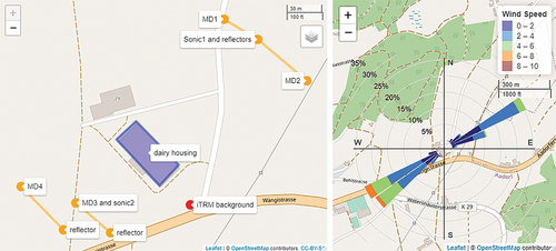
The total area of the dairy housing was 1205 m² and consisted of two compartments for 20 dairy cows each with straw mattress cubicles and a solid floor covered by a rubber mat (KURA P, Gummiwerk KRAIBURG GmbH, Tittmoning, Germany). The milking and waiting area were situated between the compartments along with other technical installations and an office. Each housing compartment was equipped with a cross channel which ran perpendicular to the building’s long axis and led to an adjacent underground slurry store to the SW of the housing and was separated from the housing compartments by rubber flaps. The slurry store consisted of two compartments (one for each housing compartment) of 252 m³ in total with a solid cover and four openings. The housing compartments were not thermally insulated. Ventilation was adjusted with flexible curtains along façades, which during the measurement periods were varied from completely open, through a combination of completely closed on the NE side and partially or completely closed on the SW side, to completely drawn on all sides. The curtains were fully closed for the last 4 days of the first measurement period and during the entire second measurement period. More information on the study site can be found in (Bühler et al. 2021; Poteko et al. 2018).

Management routines included milking twice daily (05:30 and 16:30 local time), as well as dung removal with stationary scrapers 12 times per day. During the measurements 40 primiparous and multiparous lactating Brown Swiss and Swiss Fleckvieh cows were housed in the building. The diets of the dairy cows consisted of either hay, maize pellets, and a mixture of maize and bean pellets, or grass silage, maize silage, and hay. Both diets were supplemented with concentrates individually allocated by an automatic feeder according to milk yield and lactation stage. The average body weight was 701 kg in autumn and 685 kg in winter with a mean daily milk yield of 23.2 kg and 25.7 kg, respectively. The cows had no access to the pasture or outdoor exercise areas during the experiment.

Wastewater treatment plant

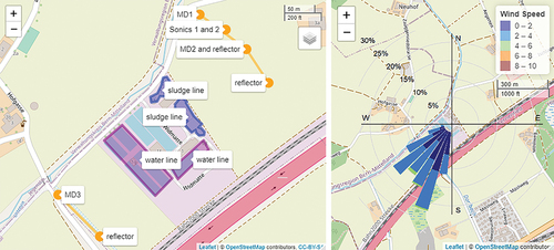
Measurements were conducted at a medium-sized WWTP (47.055620° N, 7.539515° E, 507 m altitude) which used a conventional activated sludge treatment with complete nitrification and denitrification. The plant processed waste of 43534 PE, which corresponded to 33126 connected inhabitants plus industrial waste. The site encompassed an area of 2.18 ha and consisted of multiple emitting structures totaling 5617 m² including sand traps, primary and secondary clarifiers, activated sludge tanks, thickener and digester towers (total volume of 2200 m³), a gas storage tank and open sludge storage tanks. It was selected based on the suitability of the location for IDM measurements i.e., minimal topographic obstructions (Figure 2). No large undulations or additional emission sources were present within 1 km in the dominant wind direction (SW). The plant applied conventional activated sludge treatment with complete nitrification and denitrification. The thickened sludge had a dry matter content of 4% before entering the anaerobic digester where it resided for 20 days. It was then further dewatered again to 8% dry matter content through the addition of flocculants by means of a rotary screen. Afterwards the sludge was stored in open tanks with a total volume of 1960 m³ (632 m³ in use at the time) and a surface of 331 m², which were regularly agitated typically in the morning before part of the sludge was transported to another facility for further treatment and incineration. Mean operational data during the measurement period were comparable to annual means (see Table SI2.1 for average operational data during the measurement periods). The mean incoming N load from ammonium (NH₄-N) during the measurement period was 350 kg NH₄-N d⁻¹ in total or 7.8 g NH₄-N PE⁻¹ d⁻¹ which is within the expected range for Swiss WWTPs (Kupper and Chassot 1999).

Figure 2. Map of the wastewater treatment plant with emitting structures marked on the left (blue shading for the sludge line and purple for the water line). Yellow dots and lines represent the miniDOAS sensors and measurement paths (MD1 to 3) and sonic anemometers. Wind speeds and frequencies during the measurement period are shown on the right. Map data © OpenStreetMap contributors. Please see the online version for the full colours.

Measurement campaigns

Line-integrated concentration measurements

Measurements at the dairy housing were split into two periods of 36 days (autumn) and 23 days (winter) from September to December 2018, but only one measurement period at the WWTP lasting 21 days from late September to mid-October 2019. Ammonia concentrations were measured using miniDOAS instruments placed up- and downwind of the emission sources (Figures 1 and 2). The instruments are open-path optical devices, which measure line-integrated gas concentrations between a light source and detector by UV absorption (200–230 nm wavelengths) (see Sintermann et al. 2016 for more details). The path length, here 50 m, is determined by the placement of the reflectors and the miniDOAS, which houses both the light source and detector in an environmentally controlled container. Downwind instruments were placed at a distance of approx. 10 times the maximum building height (i.e., the dairy housing was 8.5 m and the WWTP up to 15 m high) to avoid wind flow disturbance by the structures (Harper, Denmead, and Flesch 2011). At the dairy housing one set of instruments was placed 120 m NE of the building, while the second set was around 60 m SW due to topographic restrictions, while at the WWTP the up and downwind placements were 100–150 m.

In-house tracer ratio method

The measurement setup and processing is described in detail by Mohn et al. (2018) and results of the tracer release experiment for methane at this dairy housing were presented in (Bühler et al. 2021). Here the results of the NH₃ emission measurements are shown. In brief, each housing compartment was dosed with a different tracer gas (i.e., sulfur hexafluoride (SF₆) and trifluoromethyl sulfur pentafluoride (SF₅CF₃)) to identify emissions from each location. The tracer and target (NH₃) gas concentrations were concurrently quantified from a representative air sample collected in the housing using a GC-ECD and a Picarro analyzer (G2301, Picarro Inc., USA). Emissions were calculated based on the ratio of the background-corrected gas concentrations of each target to tracer gas multiplied with the dosed mass flow of the tracer gases. This method assumes that the dispersion of the tracer gas behaves the same way as the target gas and mimics its emissions (Demmers et al. 2001). The iTRM comparison measurements consisted of 2 intervals lasting 4 or 8 days during each IDM measurement period. Background concentrations were sampled 30 m SE of the housing (Figure 1). The iTRM data represented average emissions for 10 min intervals for each compartment, which were summed and then averaged to 30-min means before being compared with the corresponding 30-min IDM measurement intervals.

Meteorological measurements

Three-dimensional sonic anemometers (Gill Windmaster, Gill Instrument Ltd., Lymington, Hampshire, UK) were installed up- and downwind of the source structures at around 1.4 m height to measure the wind flow and turbulence for the bLS model and logged at 10 Hz. Since the wind direction at the dairy housing alternated between SW and NE, only data from the respective downwind sonic was used for the bLS model. Additional meteorological data (air temperature, pressure, precipitation) were obtained at both sites using an OTT WS700 weather station (OTT Hydromet GmbH, Germany) and at the dairy housing a nearby weather station (Tänikon, MeteoSwiss) provided additional meteorological data. Coordinates of the instruments and source locations are needed for the bLS model and were collected with a handheld GPS (Trimble Pro 6T, Trimble Navigation Limited, Westminster, USA). At both sites methane was also measured and the results were published in Bühler et al (2021, 2022).

Inverse dispersion modelling

Inverse dispersion modeling is a micrometeorological method to determine gaseous emissions in a downwind plume from sources of a known dimension and spatially constrained area. The concentration difference ΔC (mg m⁻³) between background levels in upwind C_BG and downwind C_DW measurements of a source is combined with the bLS model based on the measured turbulence characteristics to calculate the dispersion factor D_bLS (s m⁻³) needed to estimate an emission source strength Q in mass over time (Equation 1(1) $Q=\frac{C_{DW}-C_{BG}}{D_{bLS}}$(1) ).

(1) $Q=\frac{C_{DW}-C_{BG}}{D_{bLS}}$(1)

The bLS model based on (Flesch et al. 2004), which is a surface layer model covering distances <1 km, was used to calculate the dispersion factor (Equation 2(2) $D_{bLS}=\frac{{\left(C/E\right)}_{bLS}}{A_{source}}=\frac{1}{N_{Traj}}{\sum }_{T{D}_{inside}}\left(\frac{2}{w_0}\right)\ast \frac{1}{A_{source}}$(2) ) from the total backward trajectories of the line-integrated concentration measurements. The measurement path was approximated by a series of points spaced 1 m apart and propagated backward to the source area and hence is proportional to the ratio of the simulated concentration to the emission rate E, i.e., source strength per area, (C/E)_bLS as follows,

(2) $D_{bLS}=\frac{{\left(C/E\right)}_{bLS}}{A_{source}}=\frac{1}{N_{Traj}}{\sum }_{T{D}_{inside}}\left(\frac{2}{w_0}\right)\ast \frac{1}{A_{source}}$(2)

For each point and measurement interval 250000 backtrajectories were calculated and analyzed for touchdowns (TD_inside) within the source area (A_source), which provide the touchdown location coordinates and vertical velocity (w₀).

Trace gas emissions determined by this IDM method have previously been compared with an inhouse tracer ratio method at this dairy housing site and have been discussed in Bühler et al. (2021). Means from both methods were within the uncertainty range of the tracer method (<10%).

Deposition modelling

The bLS model modified by Häni et al. (2018) (R package bLSmodelR available at https://www.agrammon.ch/documents-to-download/blsmodelr/) was used to calculate dry deposition by multiplying the measured concentration increase with a proportionality constant called the deposition velocity (Wesely and Hicks 2000). The deposition velocity was approximated by a resistances approach (Sutton et al. 1995), whereby the velocity is the inverse of the sum of several resistances to deposition that must be overcome. These include the aerodynamic, boundary layer and canopy resistances across the surface–atmosphere interface, which vary with micrometeorological, canopy, and surface properties of the ecosystem. The first two resistances are calculated, while the latter can be either laboriously derived from models or depends on parameterizations which can vary significantly at the canopy level where the exchange processes take place (Flechard et al. 2011). Instead, a more practical approach was applied, in which the average between the possible upper and lower boundaries was used to estimate deposition. For the maximum possible deposition velocity (v_d,max), the canopy resistance was set to 0, i.e., assuming that the surface acts as a perfect sink, while the effects of boundary layer and canopy resistances on deposition were not considered for the minimum case. This method allows a simple, yet reasonable approximation of the likely deposition and corrected emissions therefore represent an average of the possible lower and upper flux magnitudes. The deposition flux F_d was modeled following Flechard et al. (2011); Häni et al. (2018) by

(3) $F_d=-v_d\ast C_{TD}$(3)

Where v_d is the deposition velocity and C_TD was the modeled concentration at the touchdown of a trajectory at the adsorbing surface. The aerodynamic resistance (R_a) usually included in the v_d calculation was omitted, since v_d was investigated for the layer between the modeled effective ground level i.e., z₀ plus the displacement height d and the adsorbing surface z₀’ and was therefore implicitly accounted for in the bLS dispersion model. Since the canopy resistance R_c was set to 0 in the maximum deposition flux model, the deposition velocity v_d was calculated as

(4) $v_d=\frac{1}{R_b+R_c}\to v_{d,max}=\frac{1}{R_b}$(4)

The boundary layer resistance R_b was calculated from Equation 5(5) $\int \underset{P_x}{\overset{\hspace{0.17em}}{\int }}\overline{uc}dydz=\sum _i{Q}_i+F_{d,\mathrm{u}\mathrm{p}\mathrm{w}}$(5) in Flechard et al. (2010) using the input variables: friction velocity u*, canopy temperature, roughness length z₀, and ambient air pressure. Although wet deposition was not taken into account, there were only few periods of rainfall or fog with valid measurements, hence the underestimation of calculated emissions during such periods is likely small. Also, the deposition of particulate NH₄⁺ was not investigated. The R package bLSmodelR was used for all of the modeling (Häni 2021).

In addition, based on the average conditions during the measurement campaign at the dairy housing, the fraction of the emission deposited within different distances (10, 20, 50, 100, 200 m) downwind of the source was modeled. From a simple mass balance perspective, the total horizontal flux through a vertical plane $P_x$ at distance $x$ which is perpendicular to the average wind direction (and sufficiently wide to capture the entire plume) will match the net flux, i.e., the sum of emissions $Q_i$ and the integrated deposition flux $F_{d,\mathrm{u}\mathrm{p}\mathrm{w}}=\int \underset{x<x_{\mathrm{p}\mathrm{l}\mathrm{a}\mathrm{n}\mathrm{e}}}{\overset{\hspace{0.17em}}{\int }}{F}_{d}dxdy$, upwind of the plane:

(5) $\int \underset{P_x}{\overset{\hspace{0.17em}}{\int }}\overline{uc}dydz=\sum _i{Q}_i+F_{d,\mathrm{u}\mathrm{p}\mathrm{w}}$(5)

Where $\overline{uc}$ is the temporal average of the product between the horizontal wind speed component along the main wind direction $u$ and the concentration $c$.

If we solely focus on a single source (and its contribution to the horizontal flux) and divide Equation 5(5) $\int \underset{P_x}{\overset{\hspace{0.17em}}{\int }}\overline{uc}dydz=\sum _i{Q}_i+F_{d,\mathrm{u}\mathrm{p}\mathrm{w}}$(5) by its source strength Q, we obtain the following relationship:

(6) $\int \underset{P_x}{\overset{\hspace{0.17em}}{\int }}\frac{\overline{uc}}{Q}dydz=1+\frac{F_{d,\mathrm{u}\mathrm{p}\mathrm{w}}}{Q}$(6)

The ratio $F_{d,\mathrm{u}\mathrm{p}\mathrm{w}}/Q$ represents the ratio between the total deposition (related to the source emission) between source and plane $P_x$ and the source emission strength. The ratio of the horizontal flux and the source strength is obtained from bLS model results as:

(7) $\frac{\overline{uc}}{Q}={\left(\frac{\overline{uc}}{E}\right)}_{bLS}{A}_{source}^{-1}$(7)

With $A_{source}$ being the area of the emitting source and E the emission rate per area. Due to biases stemming from both the discretization and the stochastic nature of the bLS model, the integral of the horizontal flux from model results without accounting for deposition will never be exactly equal to 1. Thus, Equation 5(5) $\int \underset{P_x}{\overset{\hspace{0.17em}}{\int }}\overline{uc}dydz=\sum _i{Q}_i+F_{d,\mathrm{u}\mathrm{p}\mathrm{w}}$(5) has been reformulated and discretized to provide:

(8) $\frac{F_{d,\mathrm{u}\mathrm{p}\mathrm{w}}}{Q}=A_{source}^{-1}\sum \sum \left({\left(\frac{\overline{uc}}{E}\right)}_{bLS,dep}-{\left(\frac{\overline{uc}}{E}\right)}_{bLS}\right)\mathrm{\Delta }y\mathrm{\Delta }z$(8)

Where the subscripts $bLS$ and $bLS,dep$ stand for model results without deposition and with deposition, respectively. The plane’s extensions were taken as 200 m in the crosswind direction and 80 m from model ground in the vertical direction. The discretization in the vertical was done in 20 steps on a logarithmic scale, while the discretization in the crosswind direction was equally spaced with 1 m distances.

Uncertainty analysis

The uncertainty analysis followed Bühler et al. (2021), whereby the uncertainty ε_Q of the mean IDM emission rate $\bar{Q}$_i over a time period Δt was estimated from the standard deviation SD of consecutive measurements of increasing lengths from 1 h to 45 h using the longer first measurement period at the dairy housing (Equation 9(9) ${\epsilon }_Q\left(\mathrm{\Delta }t\right)=2\ast SD\left\{\overline{Q_i}\left(\mathrm{\Delta }t\right)\right\}$(9) ) and represents the upper uncertainty boundary of the mean emission rates across the entire campaign.

(9) ${\epsilon }_Q\left(\mathrm{\Delta }t\right)=2\ast SD\left\{\overline{Q_i}\left(\mathrm{\Delta }t\right)\right\}$(9)

Since the SD included true variations of Q, such as diel variability, the uncertainty, ε_Q(Δt), corresponds to a 95% confidence interval of an assumed constant Q over time and is thus larger than the true uncertainty of the varying Q.

Data processing and assessment

For the IDM measurements, the 3D wind vectors (u, v, w) underwent two-axis coordinate rotations, corrections for a known bug affecting the w wind component of the Gill Windmaster instruments (Gill Instruments 2016), and were averaged to 30 min intervals. To correct for possible underestimation of NH₃ concentrations from loss by dry deposition the maximum dry deposition was modeled (Section 2.4), which represented an upper total emission boundary compared to the uncorrected emissions, which represented the lower boundary.

The bLS model cannot deal with periods of low wind speed, very high stability or instability, as well as extreme turbulence which are typically filtered out (Flesch et al. 2014; Gao et al. 2009; Harper, Flesch, and Wilson 2010). However, to avoid substantial data loss due to the meteorological conditions, a custom filtering procedure was applied based on observed variations of u and v, as well as literature values as described in Bühler et al. (2021). The filters at the dairy housing and the WWTP included friction velocity u* > 0.1 m s⁻¹ or >0.05 m s⁻¹ and for canopy height (z_H) and roughness length z₀, z_H / 100 < z₀ < z_H/ 3 or z₀ < 0.1, respectively, while the ratio of the SD of the along-wind (σ_u) or crosswind speeds (σ_v) to u*, i.e., σ_u/u* and σ_v/u* were < 4.5 at the dairy housing and < 6 at the WWTP, and at both sites |L| > 2 m for the Obukhov length and the Kolmogorov constant of the Lagrangian structure function was 3 <C0 < 10. Finally, only wind directions perpendicular to the instrument paths and therefore including the plume were retained (e.g., SW at the WWTP or SW and NE at the dairy housing). This resulted in 282 and 379 valid half-hourly measurements corresponding to a data loss of 80% and 62% during autumn and winter, respectively, at the dairy housing and 241 intervals at the WWTP corresponding to an average of 69% data loss. Since data loss occurred mostly at night, daytime data retention was as high as 40 to 60% (Figure SI1.2). There was a general bias toward more daytime data and greater loss at dawn and dusk due to the rapid changes in atmospheric turbulence conditions and the higher frequency of fog which obscures the sensors during these periods. The iTRM included 290 valid datapoints with corresponding 30-min IDM means for the comparison split across the autumn (190 intervals) and winter (100 intervals) measurements.

The WWTP consisted of several structures that acted as sources with different emission strengths within the general source area, therefore a relative source weighting factor w_i based on known literature values from Samuelsson et al. (2018) for a WWTP and Kupper et al. (2020) for pig slurry tanks representing the sludge storage emission was applied to each source (see Bühler et al. 2022). Each area A_i for each source emission Q_i with its corresponding modeled dispersion factor D_i was combined to a single source emission Q_tot based on the measured total concentration difference ΔC_tot

(10) $Q_{tot}=\frac{\mathrm{\Delta }{C}_{tot}}{{\sum }_{i=1}^N\left(\frac{w_{i{D}_i}}{A_i}\right)}\sum _{i=1}^N{w}_i$(10)

Welch t-tests and Pearson correlations were used to compare means and establish synchronous correlations with predictor variables, while a cross correlation function was used to investigate lagged correlations. A reduced major axis regression was used to compare the independent IDM and iTRM results. Other R packages used for data processing and plotting included ibts (Häni 2022), RgoogleMaps (Loecher and Ropkins 2015), scales (Wickham and Seidel 2020), ggplot2 (Wickham 2016), dplyr (Wickham et al. 2022), leaflet (Cheng et al. 2022) and openair (Carslaw and Ropkins 2012).

Results

Dairy housing

The meteorological conditions were generally representative for the respective seasons with mean ± standard deviation (SD) temperatures of 11.2 ± 4.6°C and 3.6 ± 4.1°C and mean monthly precipitation of 46 mm and 97 mm, respectively, for the autumn and winter periods at the dairy housing. Air temperatures were in the upper ranges during the autumn period, and there were multiple events with high wind speeds particularly during winter at the dairy housing (Figure SI1.1 and SI1.3).

NH₃ emissions and diel profiles

The mean (±SD) NH₃ emissions during the autumn and winter measurement periods are shown in Table 1 for both emissions without accounting for dry deposition, which indicated the lower emission range, and with corrections for maximum dry deposition representing the upper range. The averages of these ranges present a mean estimate of the total emissions resulting in 1.57 ± 0.59 kg NH₃ d⁻¹ and 0.81 ± 0.38 kg NH₃ d⁻¹ during autumn and winter, respectively. The concentration increase required to correct for dry deposition raised the uncorrected emissions by approx. 22% and the overall uncertainty of the IDM was 27%. This resulted in mean (± SD) corrections of the emissions to account for deposition of 0.28 ± 0.10 and 0.15 ± 0.07 kg NH₃ d⁻¹ for the autumn and winter periods, respectively, with mean modeled deposition velocities of 1.1 ± 0.52 cm s⁻¹ and 1.4 ± 0.55 cm s⁻¹. The measurement timeseries (Figure 3) presents the emissions accounting for mean deposition loss. Mean (±SD) NH₃ concentrations as measured by the miniDOAS for the entire measurement duration were 10.65 ± 6.86 μg NH₃ m⁻³ and 19.19 ± 14.23 μg NH₃ m⁻³ for up- and downwind instruments, respectively (Figure SI1.4).

Figure 3. Timeseries of NH₃ emissions including averaged deposition loss for the first (left) and second (right) measurement periods at the dairy housing.

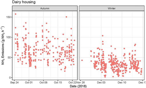
Table 1. Mean and standard deviation (SD) of non-gap filled emissions for the entire dairy housing and normalized by livestock units.

Measurement period	Type of deposition correction	Mean ± SD NH3 emissions
		(kg NH3 d^-1)	(g NH3 LU^-1 d^-1)*
Autumn	None	1.28 ± 0.5	22.8 ± 8.9
	Max	1.85 ± 0.69	33.0 ± 12.3
	Mean	1.57 ± 0.59	28.0 ± 10.5
Winter	None	0.66 ± 0.31	12.0 ± 5.6
	Max	0.97 ± 0.44	17.6 ± 8.0
	Mean	0.81 ± 0.38	14.7 ± 6.9
All	None	0.97 ± 0.40	17.6 ± 7.2
	Max	1.41 ± 0.56	25.6 ± 10.2
	Mean	1.19 ± 0.48	21.6 ± 8.7

 * Livestock units (LU = 500 kg live weight).

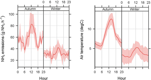
Profiles indicated a median diurnal pattern of NH₃ emissions with mean deposition corrections from the dairy housing with peak emissions during the afternoon which were more pronounced in autumn compared to winter (Figure 4). Emissions correlated best with air temperature (r = 0.51, p < 0.001), which slightly increased with a lag of 1–2 h for both periods and wind directions (up to r = 0.55, see Table SI1.1). Due to the relatively larger loss of data during the night, only the daytime emission profiles were considered robust.

Figure 4. Diurnal patterns of median NH₃ emissions with average deposition correction (left) and the mean air temperature profile (right) at the dairy housing for autumn and winter periods, respectively.

Wind sector differences

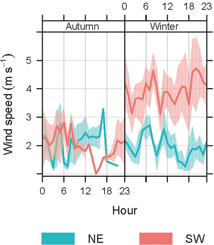
Winds were predominantly from the NE and the SW during the autumn and winter measurement periods, respectively (Figure SI1.5). Winds speeds were only higher from the SW during the winter with 3.9 ± 1.4 m s⁻¹ compared to 1.9 ± 0.6 m s⁻¹ from the NE while speeds were approx. 2.1 ± 0.8 m s⁻¹ from both directions in autumn (Figure 5). Although wind speeds were different only in winter, emissions in autumn were 20% higher with NE winds over SW winds (Figure SI1.6a). During this period, emissions additionally correlated with u* with NE but not the SW winds (Figure SI1.6b).

Figure 5. Mean diel profiles of wind speed separated by wind direction (northeast, NE, and southwest, SW) during autumn and winter periods at the dairy housing.

Comparisons with iTRM

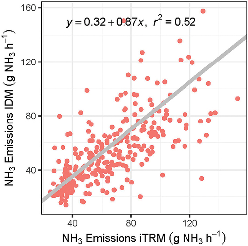
Daily averaged NH₃ emissions quantified by iTRM from both compartments were summed and compare to the entire dairy housing emissions quantified by IDM. Mean ± SD emissions by iTRM were 1.90 ± 0.58 kg NH₃ d⁻¹ and 1.00 ± 0.31 kg NH₃ d⁻¹ for autumn and winter measurements, respectively (SI Figure SI1.7). Mean IDM using only concurrent time intervals with iTRM were 1.53 ± 0.59 kg NH₃ d⁻¹ and 0.83 ± 0.34 kg NH₃ d⁻¹, hence the IDM means differed from those reported in Table 1. Therefore, mean corrected emissions by IDM for these respective periods varied up to 20% from the iTRM results (Figure 6) which represented a statistically significant difference (t-statistic = 5.73, p < 0.001).

Figure 6. Scatterplot of corresponding 30-min iTRM and IDM measurements of total NH₃ emissions (g NH₃ h⁻¹) at the dairy housing with the linear regression and coefficient of determination.

Modelled deposition loss with distance from the source

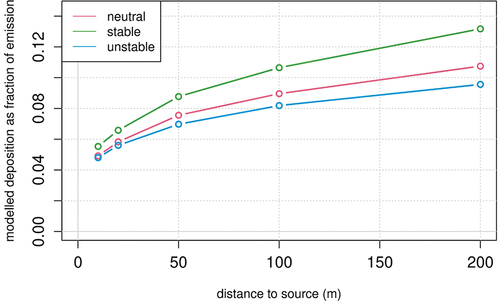
The fraction of mean deposition to emission with distance from the source based on the measurement setup at the dairy housing was highest for stable atmospheric conditions and lowest for unstable conditions (Figure 7). For each respective condition, the highest relative deposition within the first 50–150 m from the source, as relevant at our sites, ranged from 9 to 12% and 7 to 9%, respectively.

Figure 7. Relative NH₃ deposition rate as a cumulative fraction of total emissions deposited with distance from the source for different atmospheric stability conditions (defined as Obukhov length, L, −500 < L < -50 for unstable, |L| > 500 for neutral, and 10 < L < 500 for stable).

WWTP

The meteorological conditions during the measurements at the WWTP in 2019 were representative for the season with a mean ± SD temperature of 9.38 ± 2.58°C and monthly precipitation of 126 mm, albeit with periods where temperatures were in the upper ranges or with high wind speeds (Figure SI2.1).

Mean NH₃ emissions

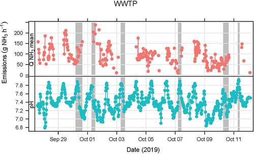
Average (mean ± SD) NH₃ emissions from the WWTP assuming no deposition loss (lower range) were 1.77 ± 0.84 kg NH₃ d⁻¹, while emissions corrected for maximum deposition (upper range) were 2.79 ± 1.28 kg NH₃ d⁻¹. Averaged emissions representing a mean corrected estimate of deposition were 2.27 ± 1.53 kg NH₃ d⁻¹ (Figure 8 top), which resulted in a deposition correction of 28% with an overall uncertainty of IDM at 24%. The per person equivalent of the mean emissions corresponded to 18.4 g NH₃ PE⁻¹ yr⁻¹, which represented 0.63% of the nitrogen (NH₄-N) inflow. The mean deposition correction for the emissions was 0.51 ± 0.23 kg NH₃ d⁻¹ and the mean deposition velocity was 0.65 ± 0.40 cm s⁻¹. Mean (±SD) concentrations as measured by the miniDOAS instruments up- and downwind of the WWTP were 4.71 ± 0.82 μg NH₃ m⁻³ and 7.19 ± 1.55 μg NH₃ m⁻³, respectively (Figure SI2.3).

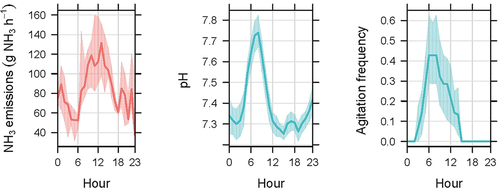
Figure 8. Timeseries of mean deposition-corrected NH₃ emissions (top) and pH (bottom) at the inflow of the WWTP with agitation events (grey shaded bars) of the slurry storage tanks during the measurement period. Note that pH, was measured at the inflow to the water line and not at the sludge tanks.

Emission responses to management activities

Although a pH above 7 increases the partitioning of NH₃ to NH₄⁺ and the temporal pattern of emissions was similar to that of pH (mean 7.4 ± 0.2) measured at the inflow (Figure 8 bottom), there was only a weak concurrent correlation (Pearson’s r = 0.15, p < 0.05). Using a cross correlation function to determine asynchronous leads and lags, statistically significant lagged relationships were found up to 5.5 h after changes in pH with peak correlations at 3 h (r = 0.52, F-statistic = 29.3, p < 0.001). All sewage sludge tank agitators were operated on Monday mornings (06:00–12:00 local time on 30^th September and 7^th October), while one tank was additionally agitated more frequently during the week. However, no direct changes in emissions could be observed in response to agitation, as the two prominent agitation events coincided with measurement gaps.

As with the dairy housing, diurnal patterns in emissions were also evident and emissions peaked again around midday lagging behind management activities affecting pH or agitation times by 3–6 h, both of which peaked early morning (Figure 9). Emissions correlated moderately with air temperature (Pearson’s r = 0.48, p < 0.001) which improved with a 3-hr offset (r = 0.75, p < 0.001), while incoming solar radiation also showed a high instantaneous correlation (r = 0.67, p < 0.001). A moderate correlation was also observed between emissions and wind speed (r = 0.30, p < 0.001).

Figure 9. Diel profiles of median NH₃ emissions with deposition corrections (left), mean pH measured at the inflow (middle), and counts of agitation events mixing the sludge tanks (right).

Discussion

Dairy housing emissions

There were up to 20% differences in IDM-based emissions between main wind directions during the autumn measurements with higher emissions for NE compared to SW winds, although these were still within the estimated uncertainty range, i.e., <27%. Increased emissions with NE winds, might have resulted from slightly higher wind speeds further indicated by the increased but still weak correlation of emissions with u* for this direction only. However, in the winter period, wind speeds were even higher from the SW but did not result in differences in emissions. A more likely explanation was the diel shift in wind direction which was observed only in autumn reflecting daily emission patterns, whereby NE winds were more prevalent during the day when emissions were higher and SW winds during the evening. However, we could not exclude the possibility that emissions may have been affected by different curtain settings, which were either half or fully open during autumn but fully closed in winter. Therefore, it is possible that the curtain settings affected the emission measurements from their position which increased aeration but also their presence affecting source geometry due to changes in turbulence conditions.

The diurnal pattern with higher daytime emissions, which was more prominent during the autumn measurement at the dairy housing, was probably mostly driven by air temperature (Bougouin et al. 2016; VanderZaag et al. 2015). Other studies found similar patterns for dairy housing emissions with daytime peaks being highest in summer, then transitional seasons and lowest in winter (Flesch et al. 2009; Saha et al. 2014). While wind speed showed no distinct diel patterns, it was higher during the winter period when emissions were lower further indicating the dominant effect of temperature compared to wind speed. This follows similar findings by Schrade et al. (2012), in which total emissions across six farms showed some correlation with wind speed but the effects of air temperature and milk urea content were more dominant. This has also been observed for different housing types and manure management systems (Bougouin et al. 2016; Liao et al. 2021; Saha et al. 2014).

The comparison of NH₃ emission estimates between IDM and iTRM showed good agreement with an overall deviation of < 20%, i.e., within the uncertainty of IDM. The possible underestimation by IDM with an averaged deposition correction may indicate that the correction was too low. In fact, the estimates with corrections for maximum deposition more closely matched emissions determined by iTRM (<3% difference). Although instrument precision and dispersion modeling may contribute to this difference, our results indicate that deposition is likely the main contributor. This conclusion agrees with results from Bühler et al. (2021) who observed smaller differences between IDM and iTRM of < 10% for methane emissions, which act as a good reference since deposition is not relevant (Lassman et al. 2020). Even though the slurry tank contributions were minor since it was covered, it is worth noting that iTRM did not include these emissions.

In terms of magnitude, our measurements were within typical ranges from the literature for loose housings with solid floors and no exercise yard during transition seasons (i.e., spring and autumn) and winter, which ranged from 3.5–92.9 g NH₃ LU⁻¹ d⁻¹ and 5.2–87.9 g NH₃ LU⁻¹ d⁻¹ , respectively (Poteko, Zähner, and Schrade 2019). Compared to ranges published by Schrade et al. (2012) in Switzerland, the IDM measurements agreed well for the respective seasons, i.e., 28.0 ± 10.5 in autumn and 14.7 ± 6.9 g NH₃ LU⁻¹ d⁻¹ in winter compared with 16–44 g NH₃ LU⁻¹ d⁻¹ and 6–23 g NH₃ LU⁻¹ d⁻¹, respectively. Other seasonal means for naturally ventilated barns with solid floors from a meta-analysis by Bougouin et al. (2016), which covered multiple measurement methods, were comparable with autumn and winter averages around 31.6 ± 4.3 and 43.5 ± 29.9 g NH₃ cow⁻¹ d⁻¹, respectively, compared to our 39.2 ± 14.7 g NH₃ cow⁻¹ d⁻¹ and 20.2 ± 9.5 g NH₃ cow⁻¹ d⁻¹ (note the different units, as LU was not available). Their winter mean emissions were higher due to two studies in the UK and USA. Including all seasons, mean annual emissions were 47.7 g NH₃ cow⁻¹ d⁻¹, therefore the autumn and winter means were a factor of 0.66 and 0.91 of the annual mean, respectively, while the seasonal weighting factors derived from means in Schrade et al. (2012) were 0.96 and 0.49, respectively. The factors of seasonal to annual mean emissions were closer to those from Schrade et al. (2012), in which winter emissions were a factor of 0.6–0.8 lower than the autumn ones, while the values in this study were 0.53 of those in autumn. Saha et al. (2014) measured seasonal averages for winter and autumn ranging between 7.9–35.3 and 5.5–54.7 g NH₃ LU⁻¹ d⁻¹ for naturally ventilated housings using the carbon dioxide balance method. Their seasonal average weightings were 0.54 and 0.75 for winter and autumn, respectively, compared to the annual mean and the mean ratio of winter to autumn, i.e., 0.71, were similar to those listed above. Although comparing very well to other studies, it is likely that our daily means had a slight bias toward higher values due to the lower representation of transitional (dawn and dusk) and nighttime periods when emissions are low because atmospheric conditions during these times deviate from the assumed ideal conditions for IDM leading to data rejection. In addition to the daily data representativeness, it is important to consider the seasonal impacts when comparing emission measurements and applying annual emission factors.

Specifically compared to other line-integrated measurements from Flesch et al. (2009) who used a bLS model and measured whole farm, as well as separate source structures by relocating the sensors, at free-stall barns also equipped with semi-drawn curtains, our measurements were in similar seasonal ranges and ratios, as their barn emissions amounted to 21.2 ± 10.7 g NH₃ animal⁻¹ d⁻¹ in autumn and 11.7 ± 10.2 g NH₃ animal⁻¹ d⁻¹ in winter. They also found similar but still weak diurnal patterns for the barns modulated only somewhat by air temperature in autumn and winter with u* being of minor importance. Moreover, they found that the management practices across the different farms were the most influential on emissions (i.e., naturally ventilated free-stall barns, sand bedding, regularly scraped barn floors) and that the same IDM technique allowed good comparisons between locations.

WWTP emissions

Total emissions at the WWTP were higher than at the dairy housing and although fewer data were available, there was a much more prominent diurnal profile. Higher emissions are expected during the day due to higher N loads in the wastewater from human activity, but also from the higher temperatures driving emissions through increased molecular diffusion of NH₃ which enhances emissions from both the sludge and water line. However, peak air temperatures were often reached in the late afternoon while emissions peaked around noon leading to the higher offset correlation. Incoming solar radiation peaked at noon and showed a high synchronous correlation with emissions. Since many of the emission sources at the WWTP had open surfaces that were exposed to the sun (especially the sludge storage tanks, but also much of the water line), localized surface heating likely facilitated this higher correlation compared to ambient air temperature. With emissions being affected by weather conditions, as with the dairy housing, it is important to consider the impact of seasonality and representativeness of the measurement period for future comparisons. The emission profile also matched changes in pH and tank agitation following a time offset of 3–5.5 hr. Although NH₃ emissions are controlled by pH which determines the speciation of volatile NH₃ and nonvolatile NH₄⁺ with even microsite variations leading to observable emission changes (Hafner, Montes, and Rotz 2013; Kim and Or 2019), the pH was measured at the inflow of the water line, which is expected to contribute only 34% to total emissions (Samuelsson et al. 2018), as opposed to the storage tanks by which point the pH will have changed. More likely, agitation of the open sludge tanks caused larger contributions to the total emission variations, as they are expected to produce the most emissions (Samuelsson et al. 2018), assuming they act as an open slurry tank (Kupper et al. 2020). However, agitation did not occur daily and regrettably, no direct effects of the agitation could be observed on emissions due to gaps in the measurements directly following the larger agitation events. Following the immediate initial emission response after disturbance in a swine slurry storage tank, Blanes-Vidal et al. (2012) observed a 1.5–3.5 h delay with a subsequent NH₃ emission increase without additional disturbance. This was explained by the development of a pH gradient during the transient-state conditions after disturbance and lasted up to 48 h. Therefore, the morning agitation of the sludge most likely promoted movement to and subsequent release of NH₃ at the surface and other buffers changing the pH profile and hence contributed to emission increases with delayed and lasting effects (Kupper et al. 2021). Longer measurement periods would be required to collect sufficient data and events to definitively determine the impact on emissions, as well as more expansive monitoring of facility parameters.

The NH₃ emissions of the WWTP (94.9 ± 44.1 g NH₃ h⁻¹) were smaller than measurements by Samuelsson et al. (2018) who reported 400 ± 100 g NH₃ h⁻¹ for a much larger WWTP (805000 PE) in Gothenburg and using individual samplings at each processing stage during the day. When normalized by PE our measurements were over 4 times higher, i.e., 18.4 g NH₃ PE⁻¹ yr⁻¹ compared to 4.3 g NH₃ PE⁻¹ yr⁻¹ at the WWTP in Gothenburg. However, that plant included an activated sludge system comprised of nitrifying trickling filters and moving bed biofilm reactors for post-denitrification, which can be effective in lowering total NH₃ levels (Colón et al. 2009; Xue et al. 2010). The sludge after digestion was also dewatered with a centrifuge without intermediate liquid storage (personal communication S. Tumlin, Gryaab AB, Gothenburg). The solids were then stored for 3 weeks in open-air stockpiles before being transported off-site. Data from Aguirre-Villegas, Larson, and Sharara (2019) on anaerobically digested dairy manure with and without solid–liquid separation using a screw press or centrifuge suggested that NH₃ emissions from the solid fraction can be lower by at least one order of magnitude compared to unseparated manure. If these findings are extrapolated to our WWTP to compare anaerobically digested liquid sewage sludge in open stores (i.e., without solid–liquid separation) with the storage of dewatered sludge in the Gothenburg plant, the discrepancy in PE normalized emissions seems plausible. Furthermore, our results come closer to the estimate by Sutton et al. (1995) of 27 g NH₃ yr⁻¹ for a WWTP in the UK.

Due to the lack of emission data from WWTPs, another comparison may be drawn with emissions from slurry stores. The matrix of sewage sludge is comparable to that of pig slurry, although it contains less NH₄⁺ and the formation of a natural surface crust is less pronounced, which is expected to enhance emissions (Kupper et al. 2020). However, sewage sludge stores are agitated more frequently than slurry tanks (Kupper, Bonjour, and Menzi 2015), likely enhancing NH₃ emissions. Emissions from slurry stores with different types of slurry and tank configurations are well documented (Kupper et al. 2020), allowing an estimation of the sewage sludge tank emissions based on pig slurry emission factors for comparable stores (i.e., 0.17 g NH₃ m⁻² h⁻¹). Upscaled to the same source area as the WWTP, these emissions would amount to 80 g NH₃ h⁻¹ which compare well with the measured emissions of 95 ± 64 g NH₃ h⁻¹, further confirming that the majority of measured emissions likely originated from the sludge storage.

Dry deposition corrections

Maximum dry deposition was modeled at both sites and the range averages between the maximum and no deposition resulted in concentration corrections of 22–28% with higher percentages at the WWTP. At the dairy housing, the correction differed with wind direction by 19% for NE winds but 27% and 23% for SW winds in autumn and winter, respectively. Although emissions were lower from the SW, atmospheric conditions were mostly stable which extended the footprint and allowed for a greater proportion of the emissions to be deposited. Since the relative correction with SW winds was greater in autumn than winter, it may be feasible that the curtain position, which was more frequently open during autumn, could have affected emission estimates by altering the turbulence conditions and hence possibly also the deposition corrections. Alternatively, the lower correction of 19% during both periods with NE winds may have resulted from the shorter measurement distance for NE emissions reducing the cumulative deposition loss. Overall, the absolute corrections were lower during winter even with higher wind speeds since temperatures and hence emissions were also low.

While both the heights of the emission source and measurements can affect the proportion deposited with distance, the bLS model assumes an emission at surface level, while the measurement heights and distances from the emission source varied between 1.2–1.7 m and 60–150 m, respectively, depending on site and direction. To estimate the relative deposition loss with distance, we modeled the fraction of deposition to emission for each stability condition for the dairy housing site. For the measurement distance of 150 m, the model indicated that <12% of the emissions were deposited during stable and <9% during unstable conditions, while minimal deposition at 50 m ranged from 7% to 9%. This proportion is in contrast to the emission correction value discussed previously, which adjusted the percent concentration loss detected at the measurement point and is different to the percent deposited to emitted gas, since the concentration-associated footprint changes the contribution weightings of both source and deposition areas.

Mean deposition velocities (i.e., the inverse of the sum of all resistances) where Rc = 0 at both sites were comparable to or lower than estimates from other studies (Aksoyoglu and Prévôt 2019; Phillips, Arya, and Aneja 2004; Schrader and Brümmer 2014) for agricultural surfaces, i.e., 0.65–1.55 cm s⁻¹ and therefore boundary layer resistances were 0.64–1.54 s cm⁻¹. The model produced highest velocities at the dairy housing with SW winds during winter when emissions were lower, but wind speeds were higher, also evident from higher correlations with u*. In contrast, Phillips, Arya, and Aneja (2004) found higher daytime v_dep in summer than winter of 3.94 ± 2.79 cm s⁻¹ and 2.41 ± 1.92 cm s⁻¹, respectively, when emissions were higher even though wind speeds were lower than in winter. The surfaces between the source and measurement paths at both sites consisted of pastures and fallow fields, which led to low roughness lengths z₀ of 0.01–0.03 ± 0.01 m. The higher value of 0.03 ± 0.01 m was only during NE winds at the dairy housing, which traversed a taller pasture.

Although most studies rely on simple resistance-based deposition models (Nemitz et al. 2000) and only few use bi-directional models with a calculated compensation point (Massad, Nemitz, and Sutton 2010; Sutton et al. 1998), the emission component downwind of a plume will be negligible for calculating the deposition loss relative to the total emission of a point source (McGinn et al. 2007). However, direct measurements of net NH₃ fluxes within the downwind plume would allow a better comparison but to date only very few data of net flux measurements are available (Swart et al. 2023 and references therein). Overall, the relative deposition values at the given measurement distances, surface roughness, stability conditions, and source heights were close to the ranges from studies including results of bi-directional models (Asman, Sutton, and Schjørring 1998; Loubet et al. 2006; Shen et al. 2016; Spindler, Teichmann, and Sutton 2001; Walker et al. 2008; Yi et al. 2021). For comparable conditions, Asman, Sutton, and Schjørring (1998) estimated a dry deposition loss within 100 m of 10% with greater amounts expected over rough surfaces with more turbulence due to higher deposition velocities. Using a N deposition model Schou et al. (2006) calculated cumulative losses from a dairy farm resulting in only 5% deposition within 100 m, 10% in 300 m, and 12% by 500 m, while Fowler et al. (1998) estimated 3–10% deposition within 300 m from a poultry farm based on a transect of concentration measurements from which the canopy resistance for the deposition model was determined by a regression fit. Estimates of dry deposition using resistance and dispersion models based on emission measurements from a hog farm in North Carolina (barns with forced ventilation and a slurry lagoon) were found to be even lower, i.e., 2.9–7% within 500 m and added up to only 16.6% with a distance of 2500 m (Bajwa, Arya, and Aneja 2008). Although pig slurries can produce slightly higher NH₃ emissions from lagoons (Kupper et al. 2020), their deposition velocities were an order of magnitude lower than observed here, which the authors explained by the tendency of the deposition model used to underpredict under the given field conditions. Another study at a pig farm in South China estimated monthly means of 4.1–14% NH₃ deposition at 500 m applying passive samplers and a multi-resistance model (Yi et al. 2021). A multiapproach study downwind of a beef feedlot in southern Alberta also found relative deposition amounts of approx. 14% at 500 m using resistance modeling and flux gradient measurements (McGinn et al. 2016), while Staebler et al. (2009) found dry deposition to account for 6–12% loss within 1 km of the same feedlot using airborne concentration measurements and a deposition model. Similarly, Shen et al. (2016) determined 8% deposition at 1 km from a feedlot in Victoria, Australia. Generally, the greater the source emissions the longer the distance of deposition (Fowler et al. 1998; Shen et al. 2016). It is worth noting that these values represent individual deposition gradients and differ from top-down estimates of total deposition budgets which include the entire surroundings of a source, which can help to reduce uncertainties at regional scales (Griffis et al. 2019). Our modeled relative deposition loss compared well with these studies but highlighted the variability due to different surface properties and estimation methods of emissions, as well as models needed to derive deposition fluxes. Hence, there is a need to further constrain deposition estimates through improved models or validation by direct measurements of deposition fluxes within emission plumes.

Overall, IDM allows continuous measurements of multiple gases such as methane and NH₃ at sub-daily resolutions with lower labor costs and without interfering with local operations, making it easily deployable for longer periods to capture a wider set of environmental and management conditions. Using line-integrated measurements also offers greater representation of emissions considering wind and dispersion impacts than point measurements. Corrections for the downwind deposition loss ideally require bi-directional modeling, which is complex with high computational demands often not accessible to practical users. Furthermore, due to the considerable reliance on parameterizations, it frequently does not yield a practical reduction in uncertainty. We demonstrated that the deposition loss can be reasonably well estimated using a simple approach to constrain total emissions that still provides meaningful information, while maintaining sufficient data quality, especially considering the need for more data from buildings or sites with multiple emission sources under a variety of conditions. These emission measurements are needed to verify inventory estimates, but more urgently, to assess potential emission reducing technologies and management methods to curb emissions (Insausti et al. 2020). Particularly when testing new strategies, it is vital that emissions are not transferred elsewhere onsite or substituted with other pollutants, e.g., greenhouse gases; therefore, whole farm or whole site emissions must be quantified. With accessible IDM modeling tools and simple deposition corrections, a wider adoption of this method could improve the data availability and implementation of emission monitoring and control strategies to achieve much needed advances to decrease NH₃ emissions and improve N use efficiency.

Conclusion

This study demonstrated the application of IDM accounting for deposition losses to determine total NH₃ emissions from large-scale structures with multiple sources, such as animal housings and WWTPs, the latter of which were the first such measurements in Switzerland. The mean deposition-corrected NH₃ emissions agreed with comparable literature data where available. Clear diurnal patterns were observed, which were likely driven by air temperature and to a smaller degree wind speed, as well as management practices with indications of lagged responses. Longer datasets spanning several months across all seasons would be required to determine the contributions of the predictor variable variations and capture more representative management activities. This could be achieved with IDM’s continuous measurement operations but can be biased toward daytime periods due to requirements of specific atmospheric and site terrain conditions.

Currently, the main limitation of IDM is the relatively high uncertainty introduced by the deposition corrections which can also limit the ability to link emissions to specific activities if the effects on emissions fall within the uncertainty. We applied a simple deposition model to correct emissions assuming maximum possible deposition, which we averaged with emissions assuming no deposition. These mean deposition-corrected IDM estimates were lower compared to a reference tracer ratio method albeit still within the overall uncertainty but possibly underestimating deposition. Even though the modeled deposition to emission fractions with distance compared well to previous studies, reducing the uncertainty of determining dry deposition or conducting validation experiments of deposition models are needed to further improve the usefulness of IDM. With improved deposition corrections and longer measurement durations, IDM provides an excellent tool to evaluate complex facility-scale NH₃ emissions needed to assess potential management activities and technologies to increase the implementation of emission abatement strategies.

Acknowledgment

Funding was obtained from the Swiss Federal Office for the Environment (Contract 00.5082.P2I R254-0652 for the dairy housing measurements and Contract 06.0091.PZ/R281-0748 for the WWTP). We thank Michael Zähner (Ruminant Nutrition and Emission Research Group, Agroscope, Tänikon), Kerstin Zeyer and Simon Wyss (Laboratory for Air Pollution/Environmental Technology, EMPA, Dübendorf) for conducting the iTRM measurements and the operators of the WWTP Moossee-Urtenenbach, specifically B. Oberer, as well as Wenzel Gruber and Tobias Bührer (Eawag) for their support. We are grateful to Markus Jocher (Climate and Agriculture Group, Agroscope, Zürich) for supporting the operation of the measurement devices. Support with modeling issues and interpretation of the data by Christof Ammann (Climate and Agriculture Group, Agroscope, Zürich) and Albrecht Neftel (NRE) is gratefully acknowledged. Finally, we thank the farmers, namely Walter Denzler, Wängi and those surrounding the WWTP for their collaboration and allowing the placement of the measurement devices.

Disclosure statement

No potential conflict of interest was reported by the author(s).

Supplementary material

Supplemental data for this paper can be accessed online at https://doi.org/10.1080/10962247.2023.2271426

Data availability statement

Due to the data volume only the 30-min averaged data that support the findings of this study are openly available in Zenodo (DOI: 10.5281/zenodo.8047581 for the dairy housing data and DOI: 10.5281/zenodo.8032908 for the WWTP data). The raw data are available from the corresponding author, AV, upon reasonable request.

Additional information

Funding

The work was supported by the Swiss Federal Office for the Environment [Contract 00.5082.P2I R254-0652 and contract 06.0091.PZ/R281-0748].

Notes on contributors

Alex C. Valach

Alex C. Valach Research Scientist in the group on Gaseous Emissions from Agriculture at the Bern University of Applied Sciences, Switzerland with a focus on trace gas flux measurements from natural ecosystems and anthropogenic sources.

Christoph Häni

Christoph Häni Research Scientist in the group on Gaseous Emissions from Agriculture at the Bern University of Applied Sciences, Switzerland focussing on dispersion modelling and emission estimation of agricultural ammonia and methane sources.

Marcel Bühler

Marcel Bühler Postdoc at the Department of Biological and Chemical Engineering at Aarhus University, Denmark researching gaseous emissions from dairy barns.

Joachim Mohn

Joachim Mohn Leader of the Emissions and Isotopes group at the Swiss Federal Laboratory for Material Science and Technology, Empa in Dübendorf, Switzerland. The group researches and provides analytical tools to quantify diffuse emissions and trace transformation pathways using isotopes.

Sabine Schrade

Sabine Schrade Project Leader in sustainable dairy production systems with the Ruminant Research Unit based at the experimental dairy barn run by the Swiss Federal Research Station Agroscope Tänikon, Switzerland.

Thomas Kupper

Thomas Kupper Leader of the group on Gaseous Emissions from Agriculture at the Bern University of Applied Sciences, Switzerland. Responsible for the Agrammon emissions model and providing the Swiss national emission inventory for ammonia emissions.

References

- Aguirre-Villegas, H.A., R.A. Larson, and M.A. Sharara. 2019. Anaerobic digestion, solid-liquid separation, and drying of dairy manure: Measuring constituents and modeling emission. Sci. Total Environ. 696:134059. doi:10.1016/j.scitotenv.2019.134059.
- Aksoyoglu, S., and A.S. Prévôt. 2019. Modelling nitrogen deposition: Dry deposition velocities on various land-use types in Switzerland. Int. J. Environ. Pollut. 64 (1/2/3):1–3. doi:10.1504/IJEP.2018.099159.
- Asman, W.A.H. 1998. Factors influencing local dry deposition of gases with special reference to ammonia. Atmos. Environ. 32 (3):415–21. doi:10.1016/S1352-2310(97)00166-0.
- Asman, W.A.H., M.A. Sutton, and J.K. Schjørring. 1998. Ammonia: Emission, atmospheric transport and deposition. New Phytol. 139 (1):27–48. doi:10.1046/j.1469-8137.1998.00180.x.
- Asman, W.A.H., and H.A. van Jaarsveld. 1992. A variable-resolution transport model applied for NHx in Europe. Atmos. Environ. 26A (3):445–64. doi:10.1016/0960-1686(92)90329-J.
- Bajwa, K.S., S.P. Arya, and V.P. Aneja. 2008. Modeling studies of ammonia dispersion and dry deposition at some hog farms in North Carolina. J. Air Waste Manag. Assoc. 58 (9):1198–207. doi:10.3155/1047-3289.58.9.1198.
- Baldé, H., A.C. VanderZaag, S.D. Burtt, C. Wagner-Riddle, L. Evans, R. Gordon, R.L. Desjardins, and J.D. MacDonald. 2018. Ammonia emissions from liquid manure storages are affected by anaerobic digestion and solid-liquid separation. Agric. For. Meteorol. 258:80–88. doi:10.1016/j.agrformet.2018.01.036.
- Blanes-Vidal, V., M. Guàrdia, X.R. Dai, and E.S. Nadimi. 2012. Emissions of NH3, CO2 and H2S during swine wastewater management: Characterization of transient emissions after air-liquid interface disturbances. Atmos. Environ. 54:408–18. doi:10.1016/j.atmosenv.2012.02.046.
- Bougouin, A., A. Leytem, J. Dijkstra, R.S. Dungan, and E. Kebreab. 2016. Nutritional and environmental effects on ammonia emissions from dairy cattle housing: A meta-analysis. J. Environ. Qual. 45 (4):1123–32. doi:10.2134/jeq2015.07.0389.
- Bühler, M., C. Häni, C. Ammann, S. Brönnimann, and T. Kupper. 2022. Using the inverse dispersion method to determine methane emissions from biogas plants and wastewater treatment plants with complex source configurations. Atmos. Environ.: X 13:100161. doi:10.1016/j.aeaoa.2022.100161.
- Bühler, M., C. Häni, C. Ammann, J. Mohn, A. Neftel, S. Schrade, M. Zähner, K. Zeyer, S. Brönnimann, and T. Kupper. 2021. Assessment of the inverse dispersion method for the determination of methane emissions from a dairy housing. Agric. For. Meteorol. 307:108501. doi:10.1016/j.agrformet.2021.108501.
- Calvet, S., R.S. Gates, G. Zhang, F. Estelles, N.W.M. Ogink, S. Pedersen, and D. Berckmans. 2013. Measuring gas emissions from livestock buildings: A review on uncertainty analysis and error sources. Biosyst. Eng. 116 (3):221–31. doi:10.1016/j.biosystemseng.2012.11.004.
- Carslaw, D.C., and K. Ropkins. 2012. Openair — an R package for air quality data analysis. Environ. Modell. Software 27-28 52–61. doi:10.1016/j.envsoft.2011.09.008.
- Cheng, J., B. Karambelkar, and Z. Xie (2022): Leaflet: Create interactive web maps with the JavaScript 'leaflet' library. R package version 2.1.1. https://CRAN.R-project.org/package=leaflet
- Colón, J., J. Martínez-Blanco, X. Gabarrell, J. Rieradevall, X. Font, A. Artola, and A. Sánchez. 2009. Performance of an industrial biofilter from a composting plant in the removal of ammonia and VOCs after material replacement. J. Chem. Technol. Biotechnol. 84 (8):1111–17. doi:10.1002/jctb.2139.
- Dai, X.-R., C.K. Saha, J.-Q. Ni, A.J. Heber, V. Blanes-Vidal, and J.L. Dunn. 2015. Characteristics of pollutant gas releases from swine, dairy, beef, and layer manure, and municipal wastewater. Water Res. 76:110–19. doi:10.1016/j.watres.2015.02.050.
- Demmers, T., V.R. Phillips, L.S. Short, L.R. Burgess, R.P. Hoxey, and C.M. Wathes. 2001. SE—structure and environment: Validation of ventilation rate measurement methods and the ammonia emission from naturally ventilated dairy and beef buildings in the United Kingdom. J. Agr. Eng. Res. 79 (1):107–16. doi:10.1006/jaer.2000.0678.
- Famulari, D., D. Fowler, K. Hargreaves, C. Milford, E. Nemitz, M.A. Sutton, and K. Weston. 2004. Measuring eddy covariance fluxes of ammonia using tunable diode laser absorption spectroscopy. Water Air Soil Pollut: Focus 4 (6):151–58. doi:10.1007/s11267-004-3025-1.
- Federal Statistical Office. 2020. Agriculture and food: Pocket statistics 2020, agriculture and forestry 07. Neuchâtel, Switzerland: Federal Statistical Office.
- Ferrara, R.M., B. Loubet, P. Di Tommasi, T. Bertolini, V. Magliulo, P. Cellier, W. Eugster, and G. Rana. 2012. Eddy covariance measurement of ammonia fluxes: Comparison of high frequency correction methodologies. Agric. For. Meteorol. 158-159:30–42. doi:10.1016/j.agrformet.2012.02.001.
- Flechard, C., R.S. Massad, B. Loubet, E. Personne, D. Simpson, J.O. Bash, E.J. Cooter, E. Nemitz, and M.A. Sutton. 2013. Advances in understanding, models and parameterizations of biosphere-atmosphere ammonia exchange. Biogeosciences 10 (7):5183–225. doi:10.5194/bg-10-5183-2013.
- Flechard, C., E. Nemitz, R.I. Smith, D. Fowler, A.T. Vermeulen, A. Bleeker, J.W. Erisman, D. Simpson, L. Zhang, Y.S. Tang, et al. 2011. Dry deposition of reactive nitrogen to European ecosystems: A comparison of inferential models across the NitroEurope network. Atmos. Chem. Phys. 11 (6):2703–28. doi:10.5194/acp-11-2703-2011.
- Flechard, C., C. Spirig, A. Neftel, and C. Ammann. 2010. The annual ammonia budget of fertilised cut grassland - part 2: Seasonal variations and compensation point modeling. Biogeosciences 7 (2):537–56. doi:10.5194/bg-7-537-2010.
- Flesch, T.K., L.A. Harper, J.M. Powell, and J.D. Wilson. 2009. Inverse-dispersion calculation of ammonia emissions from Wisconsin dairy farms. Trans. ASABE 52 (1):253–65. doi:10.13031/2013.25946.
- Flesch, T.K., S.M. McGinn, D. Chen, J.D. Wilson, and R.L. Desjardins. 2014. Data filtering for inverse dispersion emission calculations. Agric. For. Meteorol. 198-199:1–6. doi:10.1016/j.agrformet.2014.07.010.
- Flesch, T.K., X.P.C. Vergé, R.L. Desjardins, and D. Worth. 2013. Methane emissions from a swine manure tank in western Canada. Can. J. Anim. Sci. 93 (1):159–69. doi:10.4141/cjas2012-072.
- Flesch, T.K., J.D. Wilson, L.A. Harper, and B.P. Crenna. 2005. Estimating gas emissions from a farm with an inverse-dispersion technique. Atmos. Environ. 39 (27):4863–74. doi:10.1016/j.atmosenv.2005.04.032.
- Flesch, T.K., J.D. Wilson, L.A. Harper, B.P. Crenna, and R.R. Sharpe. 2004. Deducing ground-to-air emissions from observed trace gas concentrations: A field trial. J. Appl. Meteorol. 43 (3):487–502. doi:10.1175/1520-0450(2004)043<0487:DGEFOT>2.0.CO;2.
- Flesch, T. K., J.D. Wilson, L.A. Harper, R.W. Todd, and N.A. Cole. 2007. Determining ammonia emissions from a cattle feedlot with an inverse dispersion technique. Agric. For. Meteorol. 144 (1–2):139–55. doi:10.1016/j.agrformet.2007.02.006.
- Fowler, D., C. Pitcairn, M.A. Sutton, C. Flechard, B. Loubet, M. Coyle, and R.C. Munro. 1998. The mass budget of atmospheric ammonia in woodland within 1 km of livestock buildings. Environ. Pollut. 102 (1):343–48. doi:10.1016/S0269-7491(98)80053-5.
- Fowler, D., C.E. Steadman, D. Stevenson, M. Coyle, R.M. Rees, U.M. Skiba, M.A. Sutton, J.N. Cape, A.J. Dore, M. Vieno, et al. 2015. Effects of global change during the 21st century on the nitrogen cycle. Atmos. Chem. Phys. 15 (24):13849–93. doi:10.5194/acp-15-13849-2015.
- Galloway, J.N., A. Bleeker, and J.W. Erisman. 2021. The human creation and use of reactive nitrogen: A global and regional perspective. Annu. Rev. Environ. Resour. 46 (1):255–88. doi:10.1146/annurev-environ-012420-045120.
- Gao, Z., R.L. Desjardins, and T.K. Flesch. 2010. Assessment of the uncertainty of using an inverse-dispersion technique to measure methane emissions from animals in a barn and in a small pen. Atmos. Environ. 44 (26):3128–34. doi:10.1016/j.atmosenv.2010.05.032.
- Gao, Z., M. Mauder, R.L. Desjardins, T.K. Flesch, and R.P. van Haarlem. 2009. Assessment of the backward Lagrangian Stochastic dispersion technique for continuous measurements of CH4 emissions. Agric. For. Meteorol. 149 (9):1516–23. doi:10.1016/j.agrformet.2009.04.004.
- Gill Instruments. 2016. Technical key note: Software bug affecting ‘w’ wind component of the WindMaster family. Lymington, UK: Gill Instruments. http://gillinstruments.com/data/manuals/KN1509_WindMaster_WBug_info.pdf.
- Grant, R. H., M.T. Boehm, A.F. Lawrence, and A.J. Heber. 2013. Ammonia emissions from anaerobic treatment lagoons at sow and finishing farms in Oklahoma. Agric. For. Meteorol. 180:203–10. doi:10.1016/j.agrformet.2013.06.006.
- Griffis, T.J., C. Hu, J.M. Baker, J.D. Wood, D.B. Millet, M. Erickson, Z. Yu, M.J. Deventer, C. Winker, and Z. Chen. 2019. Tall tower ammonia observations and emission estimates in the U.S. Midwest. JGR Biogeosci. 124 (11):3432–47. doi:10.1029/2019JG005172.
- Hafner, S.D., F. Montes, and C.A. Rotz. 2013. The role of carbon dioxide in emission of ammonia from manure. Atmos. Environ. 66:63–71. doi:10.1016/j.atmosenv.2012.01.026.
- Häni, C., 2021. bLsmodelr: bLsmodelR - An atmospheric dispersion model in R.
- Häni, C. 2022. bLSmodelR: bLSmodelR - An atmospheric dispersion model in R. R package version 4.5-3.
- Häni, C., C. Flechard, A. Neftel, J. Sintermann, and T. Kupper. 2018. Accounting for field-scale dry deposition in backward Lagrangian stochastic dispersion modelling of NH3 emissions. Atmosphere 9 (4):146. doi:10.3390/atmos9040146.
- Harper, L.A., O.T. Denmead, and T.K. Flesch. 2011. Micrometeorological techniques for measurement of enteric greenhouse gas emissions. Anim. Feed Sci. Technol. 166-167:227–39. doi:10.1016/j.anifeedsci.2011.04.013.
- Harper, L.A., T.K. Flesch, and J.D. Wilson. 2010. Ammonia emissions from broiler production in the San Joaquin Valley. Poult. Sci. 89 (9):1802–14. doi:10.3382/ps.2010-00718.
- Hempel, S., C.K. Saha, M. Fiedler, W. Berg, C. Hansen, B. Amon, and T. Amon. 2016. Non-linear temperature dependency of ammonia and methane emissions from a naturally ventilated dairy barn. Biosyst. Eng. 145:10–21. doi:10.1016/j.biosystemseng.2016.02.006.
- Insausti, M., R. Timmis, R. Kinnersley, and M.C. Rufino. 2020. Advances in sensing ammonia from agricultural sources. Sci. Total Environ. 706:135124. doi:10.1016/j.scitotenv.2019.135124.
- Kafle, G.K., H. Joo, and P.M. Ndegwa. 2018. Sampling duration and frequency for determining emission rates from naturally ventilated dairy barns. Trans. ASABE 61 (2):681–91. doi:10.13031/trans.12543.
- Kamp, J.N., C. Häni, T. Nyord, A. Feilberg, and L.L. Sørensen. 2021. Calculation of NH3 emissions, evaluation of backward Lagrangian Stochastic dispersion model and aerodynamic gradient method. Atmosphere 12 (1):102. doi:10.3390/atmos12010102.
- Kim, M., and D. Or. 2019. Microscale pH variations during drying of soils and desert biocrusts affect HONO and NH3 emissions. Nat. Commun. 10 (1):3944. doi:10.1038/s41467-019-11956-6.
- Kupper, T., C. Bonjour, B. Achermann, B. Rihm, F. Zaucker, and H. Menzi. 2013. Ammoniakemissionen in der schweiz 1990-2010 und Prognose bis 2020, 110. Bern, Switzerland: BAFU.
- Kupper, T., C. Bonjour, and H. Menzi. 2015. Evolution of farm and manure management and their influence on ammonia emissions from agriculture in Switzerland between 1990 and 2010. Atmos. Environ. 103:215–21. doi:10.1016/j.atmosenv.2014.12.024.
- Kupper, T., and G.M. Chassot. 1999. Aufbau des Netzes zur Beobachtung des Stoffwechsels der Anthroposphäre. In Beobachtung des Stoffwechsels der Anthroposphäre im Einzugsgebiet ausgewählter Abwasserreinigungsanlagen (SEA), Ergebnisse des Projekts SEA, ed. T. Candinas and E. Bieri, 27–55. Bern: FAL - Institut für Umweltschutz und Landwirtschaft IUL Liebefeld.
- Kupper, T., R. Eugster, J. Sintermann, and C. Häni. 2021. Ammonia emissions from an uncovered dairy slurry storage tank over two years: Interactions with tank operations and meteorological conditions. Biosyst. Eng. 204:36–49. doi:10.1016/j.biosystemseng.2021.01.001.
- Kupper, T., C. Häni, A. Neftel, C. Kincaid, M. Bühler, B. Amon, and A. VanderZaag. 2020. Ammonia and greenhouse gas emissions from slurry storage - A review. Agric. Ecosyst. Environ. 300:106963. doi:10.1016/j.agee.2020.106963.
- Lassman, W., J.L. Collett, J.M. Ham, A.P. Yalin, K.B. Shonkwiler, and J.R. Pierce. 2020. Exploring new methods of estimating deposition using atmospheric concentration measurements: A modeling case study of ammonia downwind of a feedlot. Agric. For. Meteorol. 290:107989. doi:10.1016/j.agrformet.2020.107989.
- Lemes, Y.M., P. Garcia, T. Nyord, A. Feilberg, and J.N. Kamp. 2022. Full-scale Investigation of methane and ammonia mitigation by early single-dose slurry storage acidification. ACS Agric. Sci. Technol. 2 (6):1196–205. doi:10.1021/acsagscitech.2c00172.
- Lemes, Y.M., C. Häni, J.N. Kamp, and A. Feilberg. 2023. Evaluation of open- and closed-path sampling systems for the determination of emission rates of NH 3 and CH 4 with inverse dispersion modeling. Atmos. Meas. Tech. 16 (5):1295–309. doi:10.5194/amt-16-1295-2023.
- Liao, W., C. Liu, S. Jia, J. Xie, and Z. Gao. 2021. Comparing NH3 emissions under different cattle housing conditions in cold regions in China with an inverse dispersion technique. Agric. For. Meteorol. 301-302:108355. doi:10.1016/j.agrformet.2021.108355.
- Loecher, M., and K. Ropkins 2015. RgoogleMaps and loa: Unleashing R graphics power on Map Tiles. J Stat Softw 63 (4):1–18. http://www.jstatsoft.org/v63/i04/.
- Loubet, B., W.A.H. Asman, M.R. Theobald, O. Hertel, Y.S. Tang, P. Robin, M. Hassouna, U. Dämmgen, S. Génermont, P. Cellier, et al. 2009. Ammonia deposition near hot spots: Processes, models and monitoring methods. In Atmospheric ammonia, ed. M. A. Sutton, S. Reis, and S. M. H. Baker, 205–67. Netherlands, Dordrecht: Springer.
- Loubet, B., M. Carozzi, P. Voylokov, J.-P. Cohan, R. Trochard, and S. Génermont 2018. Evaluation of a new inference method for estimating ammonia volatilisation from multiple agronomic plots. Biogeosciences 15 (11):3439–60. doi:10.5194/bg-15-3439-2018.
- Loubet, B., P. Cellier, C. Milford, and M.A. Sutton. 2006. A coupled dispersion and exchange model for short-range dry deposition of atmospheric ammonia. Q. J. R. Meteorol. Soc. 132 (618):1733–63. doi:10.1256/qj.05.73.
- Massad, R.S., E. Nemitz, and M.A. Sutton. 2010. Review and parameterisation of bi-directional ammonia exchange between vegetation and the atmosphere. Atmos. Chem. Phys. 10 (21):10359–86. doi:10.5194/acp-10-10359-2010.
- McGinn, S.M., T.K. Flesch, B.P. Crenna, K.A. Beauchemin, and T. Coates. 2007. Quantifying ammonia emissions from a cattle feedlot using a dispersion model. J. Environ. Qual. 36 (6):1585–90. doi:10.2134/jeq2007.0167.
- McGinn, S.M., H.H. Janzen, T.W. Coates, K.A. Beauchemin, and T.K. Flesch. 2016. Ammonia emission from a beef cattle feedlot and its local dry deposition and re-emission. J. Environ. Qual. 45 (4):1178–85. doi:10.2134/jeq2016.01.0009.
- Mendes, L.B., N. Edouard, N.W. Ogink, H.J.C. van Dooren, I.D.F.F. Tinôco, and J. Mosquera. 2015. Spatial variability of mixing ratios of ammonia and tracer gases in a naturally ventilated dairy cow barn. Biosyst. Eng. 129:360–69. doi:10.1016/j.biosystemseng.2014.11.011.
- Mohn, J., K. Zeyer, M. Keck, M. Keller, M. Zähner, J. Poteko, L. Emmenegger, and S. Schrade. 2018. A dual tracer ratio method for comparative emission measurements in an experimental dairy housing. Atmos. Environ. 179:12–22. doi:10.1016/j.atmosenv.2018.01.057.
- Nemitz, E., M.A. Sutton, J.K. Schjoerring, S. Husted, and G. Paul Wyers. 2000. Resistance modelling of ammonia exchange over oilseed rape. Agric. For. Meteorol. 105 (4):405–25. doi:10.1016/S0168-1923(00)00206-9.
- Phillips, S.B., S.P. Arya, and V.P. Aneja. 2004. Ammonia flux and dry deposition velocity from near-surface concentration gradient measurements over a grass surface in North Carolina. Atmos. Environ. 38 (21):3469–80. doi:10.1016/j.atmosenv.2004.02.054.
- Poteko, J., M. Zähner, and S. Schrade. 2019. Effects of housing system, floor type and temperature on ammonia and methane emissions from dairy farming: A meta-analysis. Biosyst. Eng. 182:16–28. doi:10.1016/j.biosystemseng.2019.03.012.
- Poteko, J., M. Zähner, B. Steiner, and S. Schrade. 2018. Residual soiling mass after dung removal in dairy loose housings: Effect of scraping tool, floor type, dung removal frequency and season. Biosyst. Eng. 170:117–29. doi:10.1016/j.biosystemseng.2018.04.006.
- Saha, C.K., C. Ammon, W. Berg, M. Fiedler, C. Loebsin, P. Sanftleben, R. Brunsch, and T. Amon. 2014. Seasonal and diel variations of ammonia and methane emissions from a naturally ventilated dairy building and the associated factors influencing emissions. Sci. Total Environ. 468-469:53–62. doi:10.1016/j.scitotenv.2013.08.015.
- Samuelsson, J., A. Delre, S. Tumlin, S. Hadi, B. Offerle, and C. Scheutz. 2018. Optical technologies applied alongside on-site and remote approaches for climate gas emission quantification at a wastewater treatment plant. Water Res. 131:299–309. doi:10.1016/j.watres.2017.12.018.
- Schou, J.S., K. Tybirk, P. Løfstrøm, and O. Hertel. 2006. Economic and environmental analysis of buffer zones as an instrument to reduce ammonia loads to nature areas. Land Use Policy 23 (4):533–41. doi:10.1016/j.landusepol.2005.09.005.
- Schrader, F., and C. Brümmer. 2014. Land use specific ammonia deposition velocities: A review of recent studies (2004-2013). Water Air Soil Pollut. 225 (10):2114. doi:10.1007/s11270-014-2114-7.
- Schrade, S., K. Zeyer, L. Gygax, L. Emmenegger, E. Hartung, and M. Keck. 2012. Ammonia emissions and emission factors of naturally ventilated dairy housing with solid floors and an outdoor exercise area in Switzerland. Atmos. Environ. 47:183–94. doi:10.1016/j.atmosenv.2011.11.015.
- Shen, J., D. Chen, M. Bai, J. Sun, T. Coates, S.K. Lam, and Y. Li. 2016. Ammonia deposition in the neighbourhood of an intensive cattle feedlot in Victoria, Australia. Sci. Rep. 6 (1):32793. doi:10.1038/srep32793.
- Sintermann, J., K. Dietrich, C. Häni, M. Bell, M. Jocher, and A. Neftel. 2016. A miniDOAS instrument optimised for ammonia field measurements. Atmos. Meas. Tech. 9 (6):2721–34. doi:10.5194/amt-9-2721-2016.
- Sintermann, J., C. Spirig, A. Jordan, U. Kuhn, C. Ammann, and A. Neftel. 2011. Eddy covariance flux measurements of ammonia by high temperature chemical ionisation mass spectrometry. Atmos. Meas. Tech. 4 (3):599–616. doi:10.5194/amt-4-599-2011.
- Sommer, S.G., M.L. Christensen, T. Schmidt, and L.S. Jensen. 2013. Animal manure recycling. Chichester, UK: John Wiley & Sons, Ltd.
- Spindler, G., U. Teichmann, and M.A. Sutton. 2001. Ammonia dry deposition over grassland - micrometeorological flux-gradient measurements and bidirectional flux calculations using an inferential model. Q. J. R. Meteorol. Soc. 127 (573, A):795–814. doi:10.1002/qj.49712757305.
- Staebler, R.M., S.M. McGinn, B.P. Crenna, T.K. Flesch, K.L. Hayden, and S.-M. Li. 2009. Three-dimensional characterization of the ammonia plume from a beef cattle feedlot. Atmos. Environ. 43 (38):6091–99. doi:10.1016/j.atmosenv.2009.08.045.
- Sutton, M.A., J.K. Burkhardt, D. Guerin, E. Nemitz, and D. Fowler. 1998. Development of resistance models to describe measurements of bi-directional ammonia surface-atmosphere exchange. Atmos. Environ. 32 (3):473–80. doi:10.1016/S1352-2310(97)00164-7.
- Sutton, M.A., C. Milford, U. Dragosits, C.J. Place, R.J. Singles, R.I. Smith, et al. 1998. Dispersion, deposition and impacts of atmospheric ammonia: Quantifying local budgets and spatial variability. Environ. Pollut. 102 (1):349–61. doi:10.1016/S0269-7491(98)80054-7.
- Sutton, M.A., O. Oenema, J.W. Erisman, A. Leip, H. van Grinsven, and W. Winiwarter. 2011. Too much of a good thing. Nature 472 (7342):159–61. doi:10.1038/472159a.
- Sutton, M.A., C.J. Place, M. Eager, D. Fowler, and R.I. Smith. 1995. Assessment of the magnitude of ammonia emissions in the United Kingdom. Atmos. Environ. 29 (12):1393–411. doi:10.1016/1352-2310(95)00035-W.
- Sutton, M.A., J.K. Schjorring, G.P. Wyers, J.H. Duyzer, P. Ineson, and D.S. Powlson. 1995. Plant-atmosphere exchange of ammonia. Philos. Trans. R. Soc. A. 351 (1696):261–78.
- Swart, D., J. Zhang, S. van der Graaf, S. Rutledge-Jonker, A. Hensen, S. Berkhout, et al. 2023. Field comparison of two novel open-path instruments that measure dry deposition and emission of ammonia using flux-gradient and eddy covariance methods. Atmos. Meas. Tech 16 (2):529–46. doi:10.5194/amt-16-529-2023.
- Swart, D., J. Zhang, S. van der Graaf, S. Rutledge-Jonker, A. Hensen, S. Berkhout, P. Wintjen, R. van der Hoff, M. Haaima, A. Frumau, et al. 2022. Measuring dry deposition of ammonia using flux-gradient and eddy covariance methods with two novel open-path instruments, 32.
- van Damme, M., L. Clarisse, B. Franco, M.A. Sutton, J.W. Erisman, R. Wichink Kruit, M. van Zanten, S. Whitburn, J. Hadji-Lazaro, D. Hurtmans, et al. 2021. Global, regional and national trends of atmospheric ammonia derived from a decadal (2008–2018) satellite record. Environ. Res. Lett. 16 (5):55017. doi:10.1088/1748-9326/abd5e0.
- VanderZaag, A., B. Amon, S. Bittman, and T. Kuczyński. 2015. Ammonia abatement with manure storage and processing techniques. In Costs of ammonia abatement and the climate co-benefits, ed. S. Reis, C. Howard, and M. A. Sutton, 75–112. Dordrecht: Springer.
- Vendel, K., R.J. Wichink Kruit, M. Blom, P. van den Bulk, B. van Egmond, A. Frumau, S. Rutledge-Jonker, A. Hensen, and M.C. van Zanten. 2023. Dry deposition of ammonia in a coastal dune area: Measurements and modeling. Atmos. Environ. 298:119596. doi:10.1016/j.atmosenv.2023.119596.
- Walker, J.T., G. Beachley, L. Zhang, K.B. Benedict, B.C. Sive, and D.B. Schwede. 2020. A review of measurements of air-surface exchange of reactive nitrogen in natural ecosystems across North America. Sci. Total Environ. 698:133975. doi:10.1016/j.scitotenv.2019.133975.
- Walker, J., P. Spence, S. Kimbrough, and W. Robarge. 2008. Inferential model estimates of ammonia dry deposition in the vicinity of a swine production facility. Atmos. Environ. 42 (14):3407–18. doi:10.1016/j.atmosenv.2007.06.004.
- Wesely, M., and B.B. Hicks. 2000. A review of the current status of knowledge on dry deposition. Atmos. Environ. 34 (12–14):2261–82. doi:10.1016/S1352-2310(99)00467-7.
- Wickham, H. 2016. ggplot2: Elegant Graphics for Data Analysis. New York: Springer-Verlag.
- Wickham, H., R. François, L. Henry, and K. Müller 2022. Dplyr: A grammar of data manipulation. R package version 1.0.8.
- Wickham, H., and D. Seidel. 2020. scales: Scale Functions for Visualization. R package version 1.1.1. https://CRAN.R-project.org/package=scales.
- Wu, W., G. Zhang, and P. Kai. 2012. Ammonia and methane emissions from two naturally ventilated dairy cattle buildings and the influence of climatic factors on ammonia emissions. Atmos. Environ. 61:232–43. doi:10.1016/j.atmosenv.2012.07.050.
- Xue, N., Q. Wang, C. Wu, X. Sun, and W. Xie. 2010. A pilot field-scale study on biotrickling filter treatment of NH3-containing odorous gases from organic waste composting plants. J. Zhejiang Univ. Sci. A 11 (9):629–37. doi:10.1631/jzus.A1000095.
- Yi, W., J. Shen, G. Liu, J. Wang, L. Yu, Y. Li, S. Reis, and J. Wu. 2021. High NH3 deposition in the environs of a commercial fattening pig farm in central south China. Environ. Res. Lett. 16 (12):125007. doi:10.1088/1748-9326/ac3603.
- Zöll, U., C. Brümmer, F. Schrader, C. Ammann, A. Ibrom, C.R. Flechard, D.D. Nelson, M. Zahniser, and W.L. Kutsch. 2016. Surface–atmosphere exchange of ammonia over peatland using QCL-based eddy-covariance measurements and inferential modeling. Atmos. Chem. Phys. 16 (17):11283–99. doi:10.5194/acp-16-11283-2016.