First-time calculation of the spatial distribution of concentration and air quality index over South Africa using TROPOMI data

ABSTRACT

The release of toxic gases into the atmosphere may reach concentrations that can cause undesirable health, economic, or aesthetic effects. It is therefore important to monitor the amounts of pollutants injected into the atmosphere from various sources. Most countries have a ground network with multiple measuring sites and instruments, that can measure the air quality index (AQI). However, the main challenge with the networks is the low spatial coverage. In this work, satellite data is used to calculate for the first time the spatial distribution of AQI and pollutant concentration over South Africa. The TROPOspheric Monitoring Instrument (TROPOMI) onboard Sentinel-5P data is used to calculate AQI from carbon monoxide (CO), nitrogen dioxide (NO₂), ozone (O₃), and sulfur dioxide (SO₂) gases. The results that the month of June has the worst air quality distribution throughout the country, while March has the best air quality distribution. Overall, the results clearly show that TROPOMI has the capability to measure air quality at a country and city level.

Implications: In this work, satellite data is used to calculate for the first time the spatial distribution of the air quality index (AQI) and pollutant concentration over South Africa. The TROPOspheric Monitoring Instrument (TROPOMI) onboard Sentinel-5P data is used to calculate AQI from carbon monoxide (CO), nitrogen dioxide (NO₂), ozone (O3), and sulfur dioxide (SO₂) gases. Currently, South Africa has a ground network of instruments that measure AQ, however, the network does not cover the whole country. In this work, we show that the use of TROPOMI can compliment the current network and provide data for the areas not covered.

Introduction

Expanding urbanization, developing populaces and resource-intensive exercises have made most cities a noteworthy source of air contamination (Abera et al. 2021). Air contamination is one of the perilous substances that’s well known to affect perversely on the human wellbeing. Over time, human exercises such as vehicle emanations, burning of coal for power generation and fabricating of chemicals have enormously expanded the rate of air contamination. It has been found that air contamination influences those living in large urban regions where road emissions contribute the most to the debasement of air quality (Manisalidis et al. 2020). Additionally, air pollution has been shown to impact the quality of soil and water bodies by contaminating precipitation deposited into water and soil environments (Kjellstrom et al. 2006; Maipa, Alamanos, and Bezirtzoglou 2001). Wilson and Suh (1997) also showed that acid rain, global warming and the greenhouse effect have an important ecological impact on air pollution. The World Wellbeing Organization (WHO) gauges that 99% of the worldwide populace breathes unclean air, and air pollution causes 7 million untimely deaths a year (WHO 2022). Ivanov (2019) showed that a normal individual breathes in around 13,000 liters of air each day which contains toxins and is dangerous to a human wellbeing. It has been shown that pollutants can affect human health. As an example, Orellano, Reynoso, and Quaranta (2021) showed a positive association between short-term sulfur dioxide (SO₂) exposure can cause respiratory mortality. Spannhake et al. (2002) showed that high (NO₂) concentrations can lengthen and worsen common viral infections and cause severe damage to the lungs. Manisalidis et al. (2020) showed that carbon monoxide (CO) can cause direct poisoning when breathed in at high levels. On the other hand, breathing ground-level ozone can trigger a variety of health problems including chest pain, coughing, throat irritation, and congestion (Zhang, Wei, and Fang 2019). There is therefore an urgent need to drastically reduce the concentration of pollutants emitted into the atmosphere to achieve cleaner air to breath.

To improve air quality, accurate air quality measurements are needed to determine the conditions of the surrounding air. Fortunately, there exist several instruments (in-situ, space-borne and air-borne) and networks that actively measure pollutants in the atmosphere (Asher et al. 2021; Dutta, Kumar, and Dubey 2021; Grivas et al. 2020; Vijayaraghavan, Snell, and Seigneur 2008). Many countries have ambient air monitoring networks that monitor the level of pollutants in particular regions. For example, India has the System of Air Quality and Weather Forecasting And Research (SAFAR) (http://safar.tropmet.res.in/index.php?menu_id=1.), France has AIRPARIF (https://www.airparif.asso.fr/en.), and South Korea has AIRKOREA (https://www.airkorea.or.kr/eng/.) and South Africa has the South African Air Quality Information System (SAAQIS) (https://saaqis.environment.gov.za/). The only limitation with these networks is the lack of national coverage. The instruments are placed strategically at hotspots but no information is available for other parts of the country. Therefore, there exists a gap in the national measurements of air quality. In general, filling the air quality monitoring gap in low- and middle-income countries has been recognized as a global challenge (Pinder et al. 2019). This is mainly due to the large size, heavy weight, high power consumption and expensive prices of the monitoring systems (Yi et al. 2015). So, satellite air quality monitoring can be one of the solutions to address this gap.

In this work we use the Sentinel-5P products to calculate for the first time the distribution of the air quality index (AQI) and concentrations of the different pollutants over South Africa. We show (1) how the AQI varies monthly, (2) how the concentrations of pollutants vary seasonally, and (3) use the COVID-19 lockdown period as a case study to demonstrate how AQI varies.

Study area

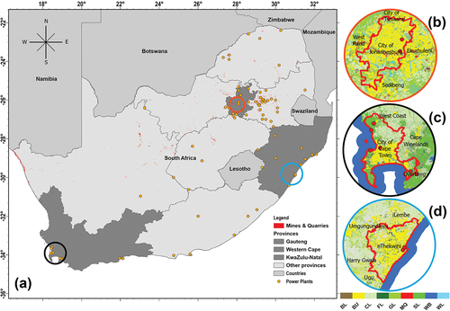
The study was conducted in South Africa, which borders Botswana, Mozambique, Namibia, Swaziland, and Zimbabwe, while Lesotho is landlocked (see Figure 1). The country has a land surface area of approximately 1,22 million km² and a population of 54,96 million. It has nine provinces, with Gauteng and Western Cape provinces being of main interest due to the high economic activity and large populations, i.e., respectively. The two provinces also host two of the three capital cities, i.e., the City of Tshwane and Cape Town, while Gauteng also hosts one of the biggest cities in Africa, i.e., Johannesburg. The climate is subtropical in the interior and temperate along the coastal areas. Generally, most of South Africa experiences summer rainfall, with an annual average of ~464 mm, while the Western Cape province is the winter-rainfall region (GCIS 2023). Figure 1 further shows the source points of emissions across South Africa. Power stations and mines appear to be the dominant sources of emissions in the country. These are concentrated in the north eastern parts of South Africa.

Figure 1. (a) a map showing the distribution of power plants and station over South Africa and the provinces of (b) Gauteng, (c) Western Cape and (d) eThekwini.

Data and method

Sentinel-5P (Precursor)

Sentinel-5P was launched on the 13^th of October 2017 with the purpose of providing operational space-borne observations and monitoring of air quality, ozone and surface UV climate. TROPOspheric Monitoring Instrument (TROPOMI) onboard Sentinel-5P is a multispectral sensor that measures the Earth’s radiance at the ultraviolet – visible (UV – VIS, 267–499 nm), near-infrared (NIR, 661–786 nm), and shortwave infrared (SWIR, 2300–2389 nm) wavelengths over ground pixels as small as 7.0 km × 3.5 km. The wavelengths are significant for measuring atmospheric concentrations of harmful substances such as aerosols, carbon monoxide (CO), nitrogen dioxide (NO₂), ozone (O₃), methane (CH₄), formaldehyde and sulfur dioxide (SO₂). TROPOMI offers data with better accuracy and at higher spatio-temporal resolution than previous instruments. More specific details on sentinel-5P can be found in Theys et al. (2017) and Tilstra et al. (2020). There are three levels of TROPOMI processing that are associated with different data products. Firstly, Level 0 products (which are not available for the public) comprise of the time-ordered, raw satellite telemetry without temporal overlap, including sensor data of the 4 spectrometers, for both atmospheric and calibration measurements. Secondly, Level-1B products comprise of geo-located and radiometrically corrected top of the atmosphere Earth radiances in all spectral bands, as well as solar irradiances. Lastly, Level-2 products consist of geo-located total columns of SO₂, NO₂, CO, O₃ CH₄ and formaldehyde. Moreover, Level-2 products consist of geo-located; (1) tropospheric columns of O₃, (2) vertical profiles of O₃, and (3) cloud and aerosol information (i.e. aerosol layer height and absorbing aerosol index). There are three types of processing requirements; near real time (NRT), Offline (OFFL), and reprocessing. NRT products are available within 3 hours after sensing, OFFL products are available within 12 hours after sensing, and for reprocessing activities there are no time constraints.

Calculation of the air quality index (AQI)

Generally, AQI is an indicator number used to report the hourly or daily air quality in an area or a locality. The primary purpose of AQI is to protect public health, especially for the health of sensitive people such as the elderly, children and asthmatics (Suman 2021). The total AQI is calculated using equation 1(1) $\mathit{AQI}=\left(I_{\mathit{P}1}+I_{\mathit{P}2}+\dots +I_{\mathit{Pn}}\right)/\mathit{n}$(1) ,

(1) $\mathit{AQI}=\left(I_{\mathit{P}1}+I_{\mathit{P}2}+\dots +I_{\mathit{Pn}}\right)/\mathit{n}$(1)

where $I_P$ is the sub-index of the concentration of the pollutant and $\mathit{n}$ is the number of pollutants. The sub-index is calculated using equation 2(2) $I_P=\frac{{\mathit{I}}_{\mathit{high}}-I_{\mathit{low}}}{C_{\mathit{high}}-C_{\mathit{low}}}\ast \left(\mathit{C}-C_{\mathit{low}}\right)+I_{\mathit{low}}$(2) ,

(2) $I_P=\frac{{\mathit{I}}_{\mathit{high}}-I_{\mathit{low}}}{C_{\mathit{high}}-C_{\mathit{low}}}\ast \left(\mathit{C}-C_{\mathit{low}}\right)+I_{\mathit{low}}$(2)

where $\mathit{C}$ is the pollutant concentration, $C_{\mathit{high}}$ is the concentration breakpoint that is ≤$\mathit{C}$, $C_{\mathit{low}}$ is the concentration breakpoint that is ≥$\mathit{C}$. $I_{\mathit{high}}$ is index breakpoint corresponding to $C_{\mathit{high}}$ and $I_{\mathit{low}}$ is index breakpoint corresponding to $C_{\mathit{low}}$. Savenets (2021) reported that the total column derived from TROPOMI cannot be truthfully estimated to near-ground values. However, the near-ground concentration value can be estimated using equation 3(3) $\mathit{C}=\frac{{\mathit{C}}_{\mathit{col}}}{\mathit{H}}.\mathit{M}.\mathit{A}$(3) ,

(3) $\mathit{C}=\frac{{\mathit{C}}_{\mathit{col}}}{\mathit{H}}.\mathit{M}.\mathit{A}$(3)

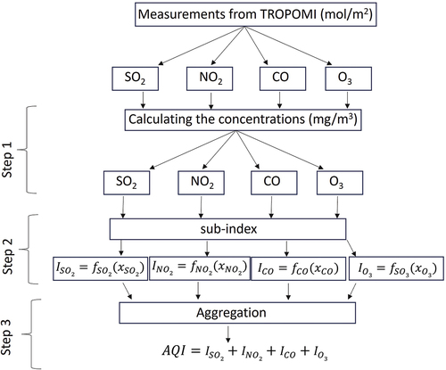
where $C_{\mathit{col}}$ is the pollutant column content (mol/m²), $\mathit{M}$ is the molar mass (g/mol), $\mathit{A}$ is a constant which is equal to 1000, for conversion from (g/m³) to (mg/m³), $\mathit{H}$ is expressed in (m). In this research, a value of H = 3000 m was chosen by assuming that most pollutants distribute in the lower troposphere. A block diagram in Figure 2 shows a summary of the calculation procedure for the AQI from TROPOMI data. Step 1 refers to the calculation of the individual pollutant concentration. The sub-index is then calculated in step 2, and the AQI is calculated in step 3.

Figure 2. A flowchart showing the calculation of the air quality index from TROPOMI.

Results and discussion

SO₂, NO₂ and CO spatial distribution concentrations

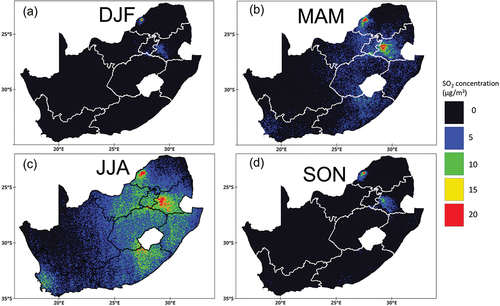
The near-surface concentrations of SO₂, NO₂ and CO are calculated from Equation 3(3) $\mathit{C}=\frac{{\mathit{C}}_{\mathit{col}}}{\mathit{H}}.\mathit{M}.\mathit{A}$(3) . The trends of SO₂, NO₂ and CO are discussed by Mokgoja, Mhangara, and Shikwambana (2023). In this study, the highest SO₂ concentration is observed during the June-July-August (JJA) winter season (see Figure 3c). During this season, the circulation patterns are strongly anti-cyclonic over most of South Africa, meaning that air masses tend to not rise, but rather settle near the ground (Masekoameng, Kornelius, and O’Beirne, 2021). The stable atmospheric conditions prevent the dilution and dispersion of air pollution, especially when emitted from sources near the surface (Cosijn and Tyson 1996). In essence, winters are characterized by the formation of surface inversion layers inhibiting vertical atmospheric mixing and effectively trapping the primary pollutants (Freiman and Piketh 2003; Lourens et al. 2011). The southwestern region of South Africa, on the other hand, experiences rainfall during the JJA period. Most of the rainfall is produced by cold fronts and associated extratropical cyclones (Singleton and Reason 2007; Xulu et al. 2023). The rainfall is responsible for the wet deposition (but not entirely) of pollutants in the atmosphere (Watson et al. 1988). Additional mechanisms of pollutant deposition involve scavenging and sedimentation, inducing downward displacement aimed at ultimately transferring pollutants to the ground surface (Watson et al. 1988). In general, for the South African context, high SO₂ concentration has mostly been observed from coal fired power stations and industrial activities (Sangeetha and Sivakumar 2019; Steyn and Kornelius 2018). Other sources of SO₂ include vehicles, especially diesel fueled vehicles (Burgard, Bishop, and Stedman 2006) and domestic solid fuel combustion (Nkosi et al. 2021). An estimated 50% or more of the total energy used in such households is allocated for cooking and space-heating (Nkosi et al. 2021). The low SO₂ concentration (<5 µg/m³) is observed in the December-January-February (DJF) (summer) and September-October-November (SON) (spring) seasons, (Figure 3a,d) respectively. The warm and wet DJF and SON seasons are associated with unstable meteorological conditions, which increase the vertical motion and dispersion in the atmosphere, thus removing most of the pollutants from the source point. Rainfall also scavenges pollutants more frequently from the atmosphere during these seasons (Lourens et al. 2011).

Figure 3. Seasonal concentration of SO₂ over South Africa for the period of 2022.

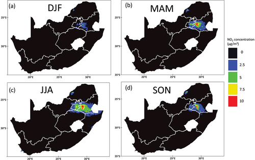
Figure 4 shows the seasonal spatial distribution of NO₂ concentration over South Africa. The DJF season (see Figure 4a) shows the lowest NO₂ concentration equal or less than 2.5 µg/m³. The low concentration is due to the unstable meteorological conditions which disperses pollutants. During the DJF season NO₂ and SO₂ in the atmosphere react with water, oxygen, and other chemicals to become sulfuric and nitric acid respectively (Parungo, Nagamoto, and Maddl 1987), thus reducing the concentrations. The reduction of the domestic fuel burning also plays a critical part in the reduction of the concentration. Moderate (5 µg/m³) to high (10 µg/m³) NO₂ concentrations are observed during the March-April-May (MAM) (see Figure 4b) and JJA (see Figure 4c) seasons in the Mpumalanga and Gauteng provinces. The stable atmospheric conditions, less rainfall and winds are responsible for the accumulation of NO₂ thus increasing its concentration. The major sources of NO₂ in these regions are coal fired power stations, and domestic solid fuel combustion, vehicle emissions (mostly petrol engines) (Nkosi et al. 2021; Wan et al. 2023), and to some extent biomass burning, which is seasonal. The SON season (see Figure 4d) shows a slight decrease in NO₂ concentration. Rainfall is usually observed in the mid SON season (Mahlalela et al. 2020), thus rainfall might be partly responsible for the slight decrease in NO₂ concentration observed during this season.

Figure 4. Seasonal concentration of NO₂ over South Africa for the period of 2022.

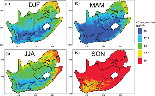
Carbon monoxide is known to play an important role in tropospheric photochemical processes and has a relatively long lifetime which ranges from weeks to months depending on the season (Toihir et al. 2015). The long lifetime of CO in the atmosphere allows it to be transported long distances from the source (Kirkman et al. 2000). The seasonal spatial distribution of CO over South Africa is shown in Figure 5. The SON season (see Figure 5d) has the highest CO concentration of 80 µg/m³ across most of South Africa except at the Western Cape province, were moderate (55–67.5 µg/m³) CO concentration is observed. The CO sources are mostly from biomass burning from fires (Shikwambana et al. 2021; Sinha et al. 2004), vehicles and machinery that burn fossil fuel. Optimal meteorological conditions of temperature, humidity, pressure, and wind speed enables the dispersion of CO during the SON season (Elbayoumi et al. 2014). The MAM season (see Figure 5b) has a low to moderate CO concentrations (30–67.5 µg/m³) across the country, however, the interior, western and southern parts of South Africa have low CO concentration. The low CO concentration in these regions could be due to strong winds (wind gust of 20 m/s or higher) which normally occur during this period (Kruger, Pillay, and van Staden 2016). The winds are likely to disperse CO rapidly in those regions. More information on the seasonal wind speed and wind distribution in South Africa can be found at Shikwambana, Mhangara, and Mbatha (2020). The DJF and JJA (see Figure 5a,c) seasons experience variability in CO concentrations across South Africa. The interior of the country comprise mostly of low to moderate CO concentrations, whereas the north eastern parts of the country comprises mostly of high CO concentrations. Shikwambana, Kganyago, and Mhangara (2023) showed that CO emissions from vehicles (especially those with diesel engines) in the South African major road networks also contribute toward the overall national average CO concentration. The northern part of the country primarily over the Limpopo province experience higher concentrations of CO during the summer and spring season presumably because the air mass transport of CO from the Congo (Central Africa) region. The results from the SAFARI 2000 campaign further shows that CO produced by biomass burning in the central Africa travels in a southward direction toward South Africa (Sinha et al. 2004; Swap et al. 2003). This increases the CO concentration in South Africa.

Figure 5. Seasonal concentration of CO over South Africa for the period of 2022.

AQI spatial distribution over South Africa

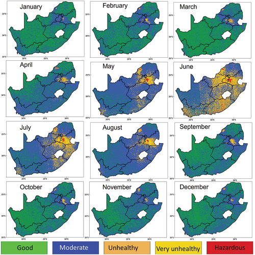
Monthly averaged spatial AQI maps for South Africa for the period of 2022 are shown in Figure 6. For this research, the air quality standard values are defined as follows; Good (0–50), moderate (50–100), uny (100–150), very unhealthy (150–300), hazardous (300–500) (USEPA 2013). In general, a lower AQI value indicates good air quality, and a higher AQI value indicates bad air quality. The results show that the Northern Cape province (27°S, 20°E) is the only region that consistently has a good and/or moderate air quality throughout the year. This province has a few mines and quarries (see Figure 1), but it does not have any coal fired power stations or huge processing factories. This province does not have big cities, and small towns that are there are far apart from each other, which lead to less AQI values. On the other hand, hazardous air quality is observed throughout the year especially some parts of the Mpumalanga province (MP) (26°S, 28°E), Limpopo province (LP) (24°S, 27°E), and the Gauteng province (GP) (26°S, 26°E). The major sources for the bad air quality in these regions are the coal fired power stations and mining activities. It is also clear from Figure 6 that the air quality is depended on the meteorological conditions of that month. Generally, the months of May, June, July and August are characterized by dry, windy and cold conditions. The stable atmospheric condition during these months prevents the drastic dispersion of pollutants from their sources, however, strong winds can transport pollutants to other regions. The month of June has the worst air quality distribution throughout the country. A study by Motlogeloa, Fitchett, and Sweijd (2023) shows that the prevalence of an outbreak of acute respiratory infectious diseases commences in May and ends in September. This finding correlates well with the bad air quality periods. The results indicate that the month of March has the best air quality distribution across the country except for some parts of MP, LP and GP. This is a transitioning period between the summer and winter seasons.

Figure 6. Monthly spatial distribution of the AQI over South Africa for the period of 2022.

Case study of AQI over cities during COVID-19 lockdown

Johannesburg

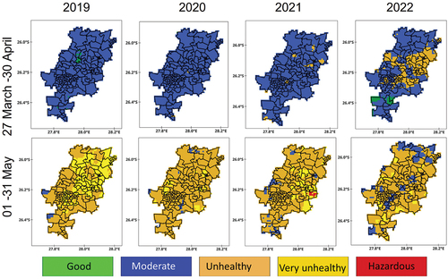
Figure 7 shows the distribution of AQI over Johannesburg for the periods: 27 March–30 April 2020 (i.e., during Level-5 lockdown) and May 01–31 May 2020 (during Level-4 lockdown). The periods of 2019, 2021 and 2022 are normal years which do not include any strict lockdown restrictions. Details of lockdown restrictions are explained in a study by Mokgoja, Mhangara, and Shikwambana (2023). Overall, the results show that the 27 March–30 April 2020 period is cleaner than the 01–31 May period. This is mostly influenced by the meteorological conditions experienced in these periods. During the period of 27 March–30 April 2020, no change in the air quality was observed compared to the 2019 period. Moderate air quality was still observed during this period. However, the in the 01–31 May period, some parts of Johannesburg’s air quality improved from very unhealthy to healthy in 2020. One of the largest sources contributing to poor air quality in Johannesburg is vehicular emissions. Johannesburg has a high population density (Brou, Shikwambana, and Sivakumar 2023), with many people owning cars. The improvement in the air quality implies a decrease in vehicle activity. Of concern is the notable decrease in the air quality from moderate to unhealthy in the eastern parts of Johannesburg during the 27 March–30 April 2022 period. The improvement in air quality in May 2020 was due to the reduction in the number of vehicles on the road. This resulted in the reduction of emissions from the vehicles. However in May 2021 there was increase in the number of vehicles on the road compared to 2020, which resulted in an increase in emissions. The temporary closure of factories and industries also contributed to the decrease in emissions in May 2020.

Figure 7. AQI distribution over Johannesburg.

Cape Town

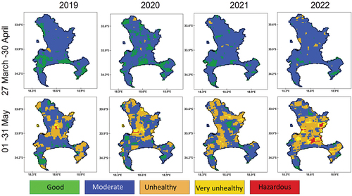
Figure 8 shows the distribution of AQI over Cape Town for the periods of 2019, 2020, 2021 and 2022. During the stricter lockdown period of 27 March–30 April 2020, improved air quality from moderate to good, especially, in central Cape Town is observed. This is due to the drastic reduction in vehicle emission on the road, manufacturing and processing factories and reduced activities at the harbor. But, this was short-lived as during the period of 01–31 May 2020 the air quality decreased in some parts of Cape Town. The degradation in air quality is linked to the lifting on of some lockdown restrictions which included operations of factories, airport and vehicles, to name a few. Similar to Johannesburg, the year 2022 has the worst air quality compared to the other years on this study. The period of 01–31 May 2022 is dominated by unhealthy air quality with some parts of the city experiencing unhealthy to hazardous conditions. The exact cause of this is not yet understood.

Figure 8. AQI distribution over Cape Town.

Durban

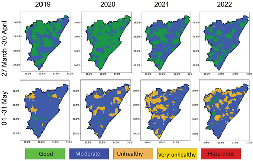
Figure 9 shows the distribution of AQI over Durban for the periods of 2019, 2020, 2021 and 2022. Overall, the period of 27 March–30 April shows a good and moderate air quality distribution across the city. However, the air quality improved during the 2020 year due to the strict lockdown restrictions, that minimized emissions. The major sources of pollutants in Durban are from vehicle emission, the harbor, airport and South Durban Industrial Basin (SDIB) which houses a large number of petroleum refineries. Mokgoja, Mhangara, and Shikwambana (2023) conducted a detailed study on the impact of the lockdown on the pollutant emissions in this region. For all the years, the period of 01–31 May sees a decrease in air quality due to the changes in the meteorological conditions in that period. Compared to 2019, a decrease in air quality in some parts of Durban is observed in 01–31 May 2020 period. It is not well understood why there was such an increase, nonetheless, the easing in the lockdown restrictions in this period is also responsible for the unexpected decrease in air quality.

Figure 9. AQI distribution over Durban.

Conclusion

It is without a doubt that air pollution has been and still is a growing concern for human health and the environment globally. Efforts by different government agencies are being made to reduce the amount of pollutants being emitted into the atmosphere in their respectful countries. In particular, the South African National Environment Management: Air Quality Act 39 of 2014 intends to (1) provide for monitoring, evaluation and reporting on the implementation of an approved pollution prevention plan, (2) create an offence for noncompliance with controlled fuels standards, and (3) provide for the establishment of the National Air Quality Advisory Committee, to name a few intentions. This study will further enforce the constitutional right (section 24 of the Bill of Rights of South Africa which states that everyone has the right: (a) to an environment that is not harmful to their health or well-being; and (b) to have the environment protected, for the benefit of present and future generations, through reasonable legislative and other measures that – (i) prevent pollution and ecological degradation; (ii) promote conservation; and (iii) secure ecologically sustainable development and use of natural resources while promoting justifiable economic and social development).

Developed countries are progressing efficiently in this regard, but developing countries such as South Africa are still making way to lower air pollution. Efforts are being made to measure and monitor air quality. The SAAQIS network has been monitoring air quality in various hot spots around the country, however, new stations have not been established in a long time, thus spatial coverage is still lacking. The use of TROPOMI data for air quality monitoring will complement the current air quality network, and provide better characterization of the spatial variability of pollutants. The results presented here clearly show that TROPOMI has the capability to measure air quality at a country and city level. With the successful demonstration of the calculation of AQI, the next step is to develop a platform which will display daily AQI for the whole of South Africa. The platform can also be used to issue out alerts for dangerous air quality events. The current limitation with the study is the poor temporal resolution of the data. TROPOMI provides daily measurements, however, for an operational system hourly measurements would be better.

Author contributions

All authors contributed to the study conception and design. Data collection and analysis were performed by Lerato Shikwambana, Nkanyiso Mbatha and Mahlatse Kganyago. The first draft of the manuscript was written by Lerato Shikwambana and all authors commented on previous versions of the manuscript. All authors read and approved the final manuscript.

Consent to publish

All authors consent to the publishing of this work.

Ethics approval and consent to participate

No ethical approval was needed for this work.

Disclosure statement

No potential conflict of interest was reported by the author(s).

Data availability statement

The data was derived from the following resources available in the public domain: Google Earth Engine, https://www.code.earthengine.google.com/.

Additional information

Notes on contributors

Lerato Shikwambana

Lerato Shikwambana is a senior scientist at the South African National Space Agency.

Mahlatse Kganyago

Mahlatse Kganyago is a senior lecturer at the University of Johannesburg.

Nkanyiso Mbatha

Nkanyiso Mbatha is the acting head of head of school of geography and a senior lecturer at the University of Zululand.

Paidamwoyo Mhangara

Paidamwoyo Mhangara is the Head of the School of Geography, Archaeology & Environmental Studies at the University of the Witwatersrand.

References

- Abera, A., J. Friberg, C. Isaxon, M. Jerrett, E. Malmqvist, C. Sjöström, T. Taj, and A. M. Vargas. 2021. Air quality in Africa: Public health implications. Annu. Rev. Public Health 42 (1):193–210. doi: 10.1146/annurev-publhealth-100119-113802.
- Asher, E., A. J. Hills, R. S. Hornbrook, S. Shertz, S. Gabbard, B. B. Stephens, D. Helmig, and E. C. Apel. 2021. Unpiloted aircraft system instrument for the rapid collection of whole air samples and measurements for environmental monitoring and air quality studies. Environ. Sci. Technol. 55 (9):5657–67. doi: 10.1021/acs.est.0c07213.
- Brou, Y. T., L. Shikwambana, and V. Sivakumar. 2023. Dynamics of Climatic and Vegetation Parameters in Urban and Township Areas: A Case Study Over the City of Johannesburg and Alexandra Township in South Africa. In Recent Advances in Environmental Sustainability. EESIWC 2021. Environmental Earth Sciences, ed. P. Li and V. Elumalai, 431–448. Cham: Springer. doi: 10.1007/978-3-031-34783-2_20.
- Burgard, D. A., G. A. Bishop, and D. H. Stedman. 2006. Remote sensing of ammonia and sulfur dioxide from on-road light duty vehicles. Environ. Sci. Technol. 40 (22):7018–22. doi: 10.1021/es061161r.
- Cosijn, C., and P. D. Tyson. 1996. Stable discontinuities in the atmosphere over South Africa. South Afr. J. Sci. 92:381–86.
- Dutta, V., S. Kumar, and D. Dubey. 2021. Recent advances in satellite mapping of global air quality: Evidences during COVID-19 pandemic. Environ. Sustain. 4 (3):469–87. doi: 10.1007/s42398-021-00166-w.
- Elbayoumi, M., N. A. Ramli, N. F. F. M. Yusof, and W. Al Madhoun. 2014. The effect of seasonal variation on indoor and outdoor carbon monoxide concentrations in Eastern Mediterranean climate. Atmos. Pollut. Res. 5 (2):315–24. doi: 10.5094/APR.2014.037.
- Freiman, M. T., and S. J. Piketh. 2003. Air transport into and out of the industrial Highveld Region of South Africa. 2002. J. Appl. Meteorol. 42 (7):994–1002. doi: 10.1175/1520-0450(2003)042<0994:ATIAOO>2.0.CO;2.
- GCIS. 2023. Accessed July 27, 2023. https://www.gcis.gov.za/content/resourcecentre/sa-info/yearbook2015-16.
- Grivas, G., E. Athanasopoulou, A. Kakouri, J. Bailey, E. Liakakou, I. Stavroulas, P. Kalkavouras, A. Bougiatioti, D. Kaskaoutis, M. Ramonet, et al. 2020. Integrating situ measurements and city scale modelling to assess the covid–19 lockdown effects on emissions and air quality in Athens, Greece. Atmosphere 11 (11):1174. doi:10.3390/atmos11111174.
- Ivanov, M. 2019. Exhaled air speed measurements of respiratory air flow, generated by ten different human subjects, under uncontrolled conditions. In E3S Web Conf, 111 02074. doi: 10.1051/e3sconf/201911102074.
- Kirkman, G. A., S. J. Piketh, M. O. Andreae, H. J. Annegarn, and G. Helas. 2000. Distribution of aerosols, ozone and carbon monoxide over southern Africa. South Afr. J. Sci. 96:423–31.
- Kjellstrom, T., M. Lodh, T. McMichael, G. Ranmuthugala, R. Shrestha, and S. Kingsland. 2006. Air and water pollution: burden and strategies for control. DCP Chap. 43:817–32.
- Kruger, A. C., D. L. Pillay, and M. van Staden. 2016. Indicative hazard profile for strong winds in South Africa. South Afr. J. Sci. 112 (1/2):01–11. doi: 10.17159/sajs.2016/20150094.
- Lourens, A. S., J. P. Beukes, P. G. van Zyl, G. D. Fourie, J. W. Burger, J. J. Pienaar, C. E. Read, and J. H. Jordaan. 2011. Spatial and temporal assessment of gaseous pollutants in the Highveld of South Africa. South Afr. J. Sci. 107 (1/2):1–8. doi: 10.4102/sajs.v107i1/2.269.
- Mahlalela, P. T., R. C. Blamey, N.C.G. Hart, and C. J. C. Reason. 2020. Drought in the Eastern Cape region of South Africa and trends in rainfall characteristics. Climate Dyn. 55 (9–10):2743–59. doi: 10.1007/s00382-020-05413-0.
- Maipa, V., Y. Alamanos, and E. Bezirtzoglou. 2001. Seasonal fluctuation of bacterial indicators in coastal waters. Microb. Ecol. Health Dis. 13:143–46. doi: 10.3402/mehd.v13i3.8016.
- Manisalidis, I., E. Stavropoulou, A. Stavropoulos, and E. Bezirtzoglou. 2020. Environmental and health impacts of air pollution: A review. Front. Public Health 8. doi: 10.3389/fpubh.2020.00014.
- Masekoameng, E., G. Kornelius, and S. O’Beirne. 2021. Introduction to the Special issue: Air quality on the South African Highveld. Clean Air J. 31. doi: 10.17159/caj/2020/31/2.12877.
- Mokgoja, B., P. Mhangara, and L. Shikwambana. 2023. Assessing the Impacts of COVID-19 on SO2, NO2, and CO trends in Durban using TROPOMI, AIRS, OMI, and MERRA-2 data. Atmosphere 14 (8):1304. doi: 10.3390/atmos14081304.
- Motlogeloa, O., J. M. Fitchett, and N. Sweijd. 2023. Defining the South African acute respiratory infectious disease season. Int. J. Env. Res. Pub. He. 20:1074. doi: 10.3390/ijerph20021074.
- Nkosi, N. C., R. P. Burger, N. R. Matandirotya, C. Pauw, and S. J. Piketh. 2021. Solid fuel use in electrified low-income residential areas in South Africa: The case of KwaDela, Mpumalanga. J. Energy South. Afr. 32 (1):58–67. doi: 10.17159/2413-3051/2021/v32i1a8086.
- Orellano, P., J. Reynoso, and N. Quaranta. 2021. Short-term exposure to sulphur dioxide (SO2) and all-cause and respiratory mortality: A systematic review and meta-analysis. Enviro. Inter. 150:106434. doi: 10.1016/j.envint.2021.106434.
- Parungo, F., C. Nagamoto, and R. Maddl. 1987. A study of the mechanisms of acid rain formation. J. Atmos. Sci. 44 (21):3162–74. doi: 10.1175/1520-0469(1987)044<3162:ASOTMO>2.0.CO;2.
- Pinder, R. W., J. M. Klopp, G. Kleiman, G. S. W. Hagler, Y. Awe, and S. Terry. 2019. Opportunities and challenges for filling the air quality data gap in low- and middle-income countries. Atmos. Environ. 215:116794. doi: 10.1016/j.atmosenv.2019.06.032.
- Sangeetha, S. K., and V. Sivakumar. 2019. Long-term temporal and spatial analysis of SO2 over Gauteng and Mpumalanga monitoring sites of South Africa. J. Atmos. Sol. Terr. Phys. 191:105044. doi: 10.1016/j.jastp.2019.05.008.
- Savenets, M. 2021. Air pollution in Ukraine: A view from the Sentinel-5P satellite. J. Hungarian Meteorolog. Serv. 125:271–90. doi: 10.28974/idojaras.2021.2.6.
- Shikwambana, L., M. Kganyago, and P. Mhangara. 2023. TROPOMI Utilized for the Monitoring of Emissions on Major Road Networks: A Case Study in South Africa During the COVID-19 Lockdown. In Recent Advances in Environmental Sustainability. EESIWC 2021. Environmental Earth Sciences, ed. P. Li and V. Elumalai. Springer, Cham. doi: 10.1007/978-3-031-34783-2_13.
- Shikwambana, L., P. Mhangara, and N. Mbatha. 2020. Trend analysis and first time observations of sulphur dioxide and nitrogen dioxide in South Africa using TROPOMI/Sentinel-5 P data. Int. J. Appl. Earth Obs. Geoinf. 91:102130. doi: 10.1016/j.jag.2020.102130.
- Shikwambana, L., X. Ncipha, S. K. Sangeetha, V. Sivakumar, and P. Mhangara. 2021. Qualitative study on the observations of emissions, transport, and the influence of climatic factors from sugarcane burning: A South African perspective. Int. J. Env. Res. Pub. He. 18 (14):7672. doi: 10.3390/ijerph18147672.
- Singleton, A. T., and C. J. C. Reason. 2007. Variability in the characteristics of cut-off low pressure systems over subtropical southern Africa. Int. J. Climatol. 27 (3):295–310. doi:10.1002/joc.1399.
- Sinha, P., L. Jaeglé, P. V. Hobbs, and Q. Liang. 2004. Transport of biomass burning emissions from southern Africa. J. Geophys. Res. 109 (D20):D20204. doi: 10.1029/2004JD005044.
- Spannhake, E. W., S. P. M. Reddy, D.B. Jacoby, X.-Y. Yu, B. Saatian, and J. Tian. 2002. Synergism between rhinovirus infection and oxidant pollutant exposure enhances airway epithelial cell cytokine production. Environ. Health Perspect. 110:665–70. doi: 10.1289/ehp.02110665.
- Steyn, M., and G. Kornelius. 2018. Authors’ Response to Letter to the Editor “An Economic assessment of SO2 reduction from industrial sources on the highveld of South Africa” by Steyn and Kornelius. Clean Air J. 28. doi: 10.17159/2410-972X/2018/v28n1a9.
- Suman, M. 2021. Air quality indices: A review of methods to interpret air quality status. Mater Today 34:863–68.
- Swap, R. J., H. J. Annegarn, J. T. Suttles, M. D. King, S. Platnick, J. L. Privette, and R. J. Scholes. 2003. Africa burning: A thematic analysis of the southern African regional science initiative (SAFARI 2000). J. Geophys. Res. 108 (D13):8465. doi: 10.1029/2003JD003747.
- Theys, N., I. De Smedt, H. Yu, T. Danckaert, J. Van Gent, C. Hörmann, T. Wagner, P. Hedelt, H. Bauer, F. Romahn, et al. 2017. Sulfur dioxide retrievals from TROPOMI onboard sentinel-5 precursor: Algorithm theoretical basis. Atmos. Meas. Tech. 10 (1):119–53. doi: 10.5194/amt-10-119-2017.
- Tilstra, L. G., M. de Graaf, P. Wang, and P. Stammes. 2020. In-orbit earth reflectance validation of TROPOMI on board the sentinel-5 precursor satellite. Atmos. Meas. Tech. 13 (8):4479–97. doi: 10.5194/amt-13-4479-2020.
- Toihir, A. M., S. Venkataraman, N. Mbatha, S. K. Sangeetha, H. Bencherif, E.-G. Brunke, and C. Labuschagne. 2015. Studies on CO variation and trends over South Africa and the Indian Ocean using TES satellite data. South Afr. J. Sci. 111 (9/10):01–09. doi: 10.17159/SAJS.2015/20140174.
- USEPA. 2013. Technical Assistance Document for the Reporting of Daily Air Quality—The Air Quality Index (AQI). 1–28, United States Environmental Protection Agency, Durham, NC.
- Vijayaraghavan, K., H. E. Snell, and C. Seigneur. 2008. Practical aspects of using satellite data in air quality modeling. Environ. Sci. Technol. 42 (22):8187–92. doi: 10.1021/es7031339.
- Wan, N., X. Xiong, G. J. Kluitenberg, J. M. S. Hutchinson, R. Aiken, H. Zhao, and X. Lin. 2023. Estimation of biomass burning emission of NO2 and CO from 2019–2020 Australia fires based on satellite observations. Atmos. Chem. Phys. 23 (1):711–24. doi: 10.5194/acp-23-711-2023.
- Watson, A.Y., R.R. Bates, D. Kennedy, eds. 1988. Atmospheric Transport and Dispersion of Air Pollutants Associated with Vehicular Emissions. In Air Pollution, the Automobile, and Public Health, 1–692. (WA, DC): National Academies Press (US). https://www.ncbi.nlm.nih.gov/books/NBK218142/.
- WHO. 2022. Accessed August 8, 2023. https://www.who.int/news/item/04-04-2022-billions-of-people-still-breathe-unhealthy-air-new-who-data.
- Wilson, W. E., and H. H. Suh. 1997. Fine particles and coarse particles: Concentration relationships relevant to epidemiologic studies. J. Air Waste Manag. Assoc. 47 (12):1238–49. doi: 10.1080/10473289.1997.10464074.
- Xulu, N. G., H. Chikoore, M.-J. M. Bopape, T. Ndarana, T. P. Muofhe, I. L. Mbokodo, R. B. Munyai, M. V. Singo, T. Mohomi, S. M. S. Mbatha, et al. 2023. Cut-Off Lows over South Africa: A Review. Climate. 11 (3):59. doi: 10.3390/cli11030059.
- Yi, W. Y., K. M. Lo, T. Mak, K. S. Leung, Y. Leung, and M. L. Meng. 2015. A survey of wireless sensor network based air pollution monitoring systems. Sensors. 15:31392–427. doi: 10.3390/s151229859.
- Zhang, J. J., Y. Wei, and Z. Fang. 2019. Ozone pollution: A major health hazard worldwide. Front Immunol. 10:2518. doi: 10.3389/fimmu.2019.02518.