Spatiotemporal change in duration of households with every member out-of-home: a case in Kumamoto, Japan

ABSTRACT

Nobody-at-home situations can cause several problems, such as home-delivery failures and burglaries. A recent study demonstrated temporal profiles of households with every member out-of-home (HEMO) situation by using household travel surveys. However, the spatial distribution of HEMO and its transition were not examined, and the effect of household attributes on HEMO was not analyzed statistically. In this study, the spatiotemporal variation in HEMO duration was investigated to address this gap, and the duration was analyzed using two econometric models. The 1984, 1997, and 2012 household travel surveys from Kumamoto, Japan, were used for the spatiotemporal visualization. In addition, the Tobit model and time allocation model were developed to statistically determine the reason for the variation in duration. The average HEMO duration increased by more than 1 h between 1984 and 2012. The downtown area revealed a longer HEMO duration, and the area with a longer duration expanded to rural areas between 1984 and 2012. The estimated econometric models revealed the statistical impacts of household attributes on HEMO duration. The HEMO duration of single-person households with a worker or student was long, and that of households with a working husband and homemaker wife was short. The spatiotemporal distribution of HEMO durations presented in this paper has the potential to be used in future urban studies, including those on the logistics of home-delivery, home-visiting survey design, crime prevention, and energy research.

KEYWORDS:

• Household occupancy
• household travel survey
• Tobit model
• time allocation model

Highlights

• Nobody-at-home duration is explored using multi-year household travel surveys.

• Average HEMO duration increased by >1 h from 1984 to 2012 in Kumamoto, Japan.

• The spatial variations in the duration throughout the year are demonstrated.

• Tobit and time allocation models explain the duration and its change.

1. Introduction

Several problems occur when nobody is at home, or every member of a household is out-of-home, including home-delivery failures and home burglaries. Home-delivery failures are a world-wide problem that causes additional labour costs, traffic, and environmental emissions (Buldeo Rai, Verlinde, & Macharis, 2021; Van Duin, De Goffau, Wiegmans, Tavasszy, & Saes, 2016). Home burglaries are also a social problem that normally occurs when nobody is at home. The nobody-at-home situation also makes a home-based interview survey difficult, making it necessary for surveyors to revisit a target household several times, which increases the survey cost and can reduce the survey quality as a result of the lower response rate. Meanwhile, the nobody-at-home situation also has certain advantages. It will reduce household energy consumption and may enable temporary accommodation by creating temporary living space in the emerging sharing economy (Hossain, 2020).

Interestingly, the nobody-at-home situation has not been fully explored in the literature. Several crime-prevention studies have used a small amount of sample data to develop burglary-incidence models using the nobody-at-home variable (Tseloni, Wittebrood, Farrell, & Pease, 2004; Wilcox, Madensen, & Tillyer, 2007). The literature on energy research has used time-use survey data and smart-metre data to detect the nobody-at-home situation (Kleiminger, Mattern, & Santini, 2014). However, the examination has usually been conducted using a single-time period survey with a limited sample size. Thus, the spatial distribution, its transition, and the effects of household attributes on the nobody-at-home situation have not been fully clarified.

Recently, Maruyama and Fukahori (2020) proposed a method to use household travel survey data to examine the nobody-at-home situation. They created temporal profiles of households with every member out-of-home (HEMO) using the 1984, 1997, and 2012 household travel surveys from Kumamoto, Japan. Furthermore, Fukahori and Maruyama (2021) explored the evolution of the temporal profiles across Japanese cities using national household travel survey data. Although a household travel survey mainly investigates travel behaviour (Calvo, Eboli, Forciniti, & Mazzulla, 2019; Kuhnimhof et al., 2012; Stopher & Greaves, 2007), it can also be used to examine the out-of-home situation using trip departure and arrival times of home-related trips. The survey collects the travel behaviour data of every member of a household; thus, it can show the temporal profiles of HEMO rates.

While Maruyama and Fukahori (2020) examined the HEMO rate, the current study investigated the HEMO duration—the total time in which every member of a household was away from home. Specifically, the study investigated the HEMO duration using the 1984, 1997, and 2012 household travel surveys from Kumamoto, Japan. These household travel surveys are called person trip (PT) surveys in Japan, and the data from the Kumamoto PT surveys were used for this study. As later shown, analyzing the HEMO duration demonstrated the spatial distribution of the results more clearly than a temporal profile analysis of the HEMO rate and made it possible to develop several statistical and econometric models.

Analyzing the HEMO situation has several prospects for further studies. Visualizing the spatial distribution of HEMO duration can provide a novel vitality map of urban areas. This map differs from the existing population density or household size distribution maps. It is also different from the dynamic population mapping using mobile phone data (e.g. Deville et al., 2014), which is individual-based. The HEMO duration map utilizes two unique features of household travel surveys: the surveys record the behaviour pattern of every household member, and their sample size is large. In urban science, the map can be considered as a base map for urban analysis (e.g. area comparison within a city and intercity comparison); however, we found no studies demonstrating it.

In addition, smart metres and other sensing technologies are speculated to estimate the HEMO profile and durations in a precise manner. Comparing them with those produced by household travel survey data will be useful in examining the possible bias in travel survey data.

Notably, home-delivery failures, which is a typical problem due to the nobody-at-home situation, may be solved by new services such as the buy-online and pick-up-at-store (Kim, Han, Jang, & Shin, 2020) and alternative delivery locations (Kim & Wang, 2022; Van Duin, Wiegmans, Van Arem, & Van Amstel, 2020). However, investigating HEMO will provide other solutions. Home-visiting survey will remain a useful method to recruit and interview participants. The HEMO profile and duration distribution will be useful in determining the timing and routing for designing an efficient visiting survey. Furthermore, HEMO distribution can be used as a base map for designing shared residential parking (Lai, Cai, & Hu, 2021; Shao, Yang, Zhang, & Ke, 2016; Xu, Cheng, Kong, Yang, & Huang, 2016; Zhang & Chen, 2021; Zhang, Liu, Wang, & Yang, 2020). Therefore, we propose that analysis of HEMO using travel survey data is important and has significant potential for future studies.

This study examined the HEMO duration using the 1984, 1997, and 2012 PT surveys from Kumamoto, Japan and demonstrating the following: the transition of the HEMO duration and durations of several household types over the 28 year period; the spatial distribution of the HEMO duration and its transition, i.e. the spatiotemporal change in the HEMO duration, over 28 years; and the factors in the HEMO duration change based on statistical and econometric modelling, i.e. Tobit and time allocation modelling.

It was found that the average HEMO duration increased by more than 1 h over the 28 year period, and main factors were increases in the numbers of single households and active seniors. The downtown area had a longer HEMO duration, and the area with a longer duration expanded to rural areas over the 28 years. These findings enhanced the findings by Maruyama and Fukahori (2020), who analyzed the temporal profiles of the HEMO rate using the same data, using geographical visualization and statistical modelling.

This paper is organized as follows. Section 2 reviews the existing literature related to the HEMO analysis. Section 3 defines the HEMO duration and shows the modelling framework. Section 4 describes the 1984, 1997, and 2012 Kumamoto PT survey data. Section 5 demonstrates the results, which is followed by a discussion in section 5. Section 6 concludes the paper.

2. Literature review

The individual-based out-of-home times have been analyzed and modelled extensively. Many studies have explored the individual-based tradeoff between in-home and out-of-home time use (Bhat & Misra, 1999; Kitamura, 1984; Meloni, Guala, & Loddo, 2004; Yamamoto & Kitamura, 1999); the choice between in-home and out-of-home activity locations (Akar, Clifton, & Doherty, 2011); the relationship between the out-of-home time, travel time, and subjective well-being (Morris, 2015); the in-home activity type and duration (Shabanpour, Golshani, Fasihozaman Langerudi, & Mohammadian, 2018a); the relationship between the well-being of the elderly and their time-usage (Enam, Konduri, Eluru, & Ravulaparthy, 2018); multi-week time-use behaviour (Spissu, Pinjari, Bhat, Pendyala, & Axhausen, 2009); the time allocation difference in generations (Enam & Konduri, 2018; Garikapati, Pendyala, Morris, Mokhtarian, & McDonald, 2016); the seniors’ driving status and out-of-home activity participation (Spinney, Newbold, Scott, Vrkljan, & Grenier, 2020); and the activity-travel time use comparison across cities (Fu, 2020).

Other studies have examined the household interaction during in-home and out-of-home activity participation (Srinivasan & Bhat, 2005); the intra-household interaction during out-of-home activity participation (Feng, Chuai, Lu, Guo, & Yuan, 2020); the time-use and activity of dual-earner couples (Bernardo, Paleti, Hoklas, & Bhat, 2015); and those of retired and working couples (Lai, Lam, Su, & Fu, 2019). Other researchers developed a comprehensive model to analyze the activity participation and duration, including the intrahousehold interaction (Bhat et al., 2013), and examined the social network and social capital impacts on the activity type and duration (Calastri, Hess, Daly, & Carrasco, 2017). Surprisingly, as far as we know, no studies have fully investigated the HEMO duration, although the concept is simple.

A few studies have examined concepts related to the HEMO duration. Miwa, Yamamoto, and Morikawa (2009) examined household shared times using the National PT survey data in Japan. The household shared time is defined as the time in which every member of a household is in the same location. Miwa et al. (2009) showed that the household shared time in a metropolitan area is shorter than that in a rural area; the shared time tends to increase over time due to increasing senior households; and the time is affected by the occupation of the head of the household, number of senior and young members, and commuting time. They used the time allocation model by Kitamura (1984) to explore the issue. Yamamoto, Miwa, and Morikawa (2009) combined PT survey data and time-use data to examine the household out-of-home shared time and revealed that regional characteristics and household income affected the shared time. The household shared time can be contrasted with the HEMO duration, but the HEMO duration was not examined even in these studies, indicating a clear research gap.

Many studies demonstrated spatiotemporal visualization related to transportation data, but no analysis of the spatiotemporal distribution of HEMO duration has been reported. Several studies have demonstrated geospatial travel features in metropolitan areas using the accessibility concept (Kelobonye et al., 2019, 2020). Currently, large-scale spatiotemporal individual trajectories are observed using the global positioning system (GPS) and other devices. Several studies analyzed taxi GPS data (Wang, Huang, Ni, & Zeng, 2019), shared public bicycle records (Cazabet, Jensen, & Borgnat, 2018; Chen & Jiang, 2021), smart card data (S. Liu, Yamamoto et al., 2021; Shi et al., 2020), and GPS-based activity diary survey (Zhang, Ji, Yu, Zhao, & Chai, 2021). However, we found no paper that reported the spatiotemporal distribution of HEMO duration.

Time-use data are widely used in energy research to explore occupant behaviour. Several studies used the American Time Use Survey to cluster the activity pattern of occupants (Diao, Sun, Chen, & Chen, 2017); and revealed that Americans spent more time at home in 2012 compared to that in 2003, and estimated the change in energy consumption (Sekar, Williams, & Chen, 2018). Other studies used the French time-use survey to explore the variation of activity duration by the household income, household composition, and housing type (De Lauretis, Ghersi, & Cayla, 2017); used the UK time-use survey to develop the activity profile of occupants (Aragon, Gauthier, Warren, James, & Anderson, 2019), and explore the change in temporal patterns of activities over 40 years (Anderson & Torriti, 2018); used the Danish Time Use survey to explore the activity profiles and the variation of activity time by season, weekday/weekend, and household composition (Barthelmes et al., 2018). Activity duration, type, and locations are also modelled for energy studies (Rovira, Imani, Sivakumar, & Pawlak, 2022). Note that the occupancy detection methods using several sensor data were intensively investigated (Tan et al., 2022); therefore, the precise estimation of occupancy duration may be possible in the future. However, even in energy research, we found no studies that fully examined or demonstrated the spatiotemporal distribution of HEMO duration.

In summary, time use has been extensively studied in transportation and energy research. Although studies demonstrated in-depth analyses of the time-use of household members, we found no studies that have fully investigated the simple synthesis of household time-use—the HEMO duration.

3. Methods

3.1. Concept and calculation of HEMO duration

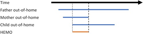
Similar to the work of Maruyama and Fukahori (2020), this study defined the ‘out-of-home duration’ as the duration between the departure from the home and the arrival time when returning home. Thus, the individual-based out-of-home durations (IO durations) can be illustrated by the lengths of the blue bars in Figure 1. The HEMO duration is defined as the duration in which every household member is out-of-home, which is illustrated by the length of the red bar in Figure 1. Maruyama and Fukahori (2020) determined the out-of-home situation in 10 min intervals, and this study also calculates the IO and HEMO durations in 10 min intervals to make the results comparable to their results.

Figure 1. Illustration of household with every member out-of-home (HEMO). Source: Maruyama and Fukahori (2020).

3.2. Tobit model formulation

This study adopted two econometric models to analyze the HEMO duration. In selecting these models, special attention was given to the features of the HEMO duration. These values are non-negative and contain many zeros. An ordinary multiple regression analysis would not be appropriate in this case. The first model was a Tobit model (Tobin, 1958), which presents nonnegative dependent variable $y_i$ of sample i as shown below: (1) $y_i^{\ast }=\beta x_i^{}+u_i,$(1) (2) $y_i^{}=\{\begin{array}{cc}{y}_i^{\ast },& y_i^{\ast }>0\\ 0,& y_i^{\ast }\le 0\end{array}i=1,2,\dots ,N,$(2) where $x_i^{}$ is the observed independent variable vector, $\beta$ is the unknown parameter vector, and N is the sample size. This study assumed that error term$u_i$ followed a normal distribution, $N(0,{\sigma }_1^2)$, and estimated parameters using the maximum likelihood method. The likelihood function is defined as below: (3) $L(\beta ,{\sigma }^2)=\prod _{y_i=0}\left\{1-\mathrm{\Phi }\left({\displaystyle \frac{\beta x_i^{}}{{\sigma }_1}}\right)\right\}\prod _{y_i>0}{\sigma }^{-1}\varphi \left\{{\displaystyle \frac{y_i-\beta x_i^{}}{{\sigma }_1}}\right\}$(3) where $\varphi (.)$ and $\mathrm{\Phi }(.)$ are the density and cumulative distribution function of a standard normal distribution, and ${\sigma }_1$ are the parameters to be estimated. The Tobit model is also called a truncated or censored regression model in some literature (Washington, Karlaftis, Mannering, & Anastasopoulos, 2020).

3.3. Time allocation model formulation

The second model was the time allocation model proposed by Kitamura (1984). Following Yamamoto et al. (2009), and Miwa et al. (2009), the formulation is shown below. First, the time use of the household is divided into the time with every member out-of-home (HEMO duration) $(j=1)$ and time with at least one member in-home (non-HEMO duration) $(j=2)$. The time allocation behaviour is expressed as the utility maximization problem. (4) $\mathrm{Maximize}U(t_1,t_2)=U_1(t_1,x_1)+U_2(t_2,x_2)$(4) $\mathrm{subject}\mathrm{to}T=t_1+t_2,$where $T$ is the total amount of time (24 h), $t_j$ is the time allocated to $j$, $x_j$ is an explanatory variable vector, and $U_j$ is the utility by $j$ ($j=1,2$). Here, the household notation is omitted for simplicity. Following Kitamura (1984), HEMO duration $t_1$ is expressed as follows using activity indicator$I_1$. (5) $t_1=\{\begin{array}{cc}0,& \mathrm{if}{I}_1\le 0\\ {\displaystyle \frac{\exp (\beta x+\epsilon )}{1+\exp (\beta x+\epsilon )}T,}& \mathrm{if}{I}_1>0\end{array}$(5) where (6) $I_1=-\ln \nu +\beta x+\epsilon ,$(6) (7) $\nu \ln T\nu -(1+\nu )\ln (1+\nu )=0.$(7)

The assumption of $T=24$ (h) leads to $\nu =0.12$ by Eq. (7). If it is assumed that error term $\epsilon \sim N(0,{\sigma }_2^2)$, the likelihood function is as follows. (8) $L=\prod _{t_1=0}\mathrm{\Phi }\left({\displaystyle \frac{\ln (\nu )-\beta x}{{\sigma }_2}}\right)\prod _{t_1>0}{\displaystyle \frac{1}{\sigma }\varphi \left({\displaystyle \frac{\ln (t_1/t_2)-\beta x}{{\sigma }_2}}\right),}$(8) where$\varphi (.)$ and $\mathrm{\Phi }(.)$ are again the standard normal density and distribution function, and ${\sigma }_2$ is the unknown parameter for the error term.

4. Data

The data used were the same as the data used by Maruyama and Fukahori (2020), from the 1984, 1997, and 2012 Kumamoto PT surveys in Japan. Table 1 gives an outline of each survey. The target area was the Kumamoto metropolitan area—Kumamoto City and its surrounding areas—and the sizes of the areas covered were almost identical in all three surveys. The survey target was every household member that was 5 years of age and older. Samples that met the following criteria, which were the same as those used by Maruyama and Fukahori (2020), were excluded from the analysis because their HEMO durations could not be calculated: either the departure time of their first trip from home, the arrival time from the trip returning home, or the departure times of trips following the trip returning home were unknown. The filtered sample size and descriptive statistics are listed in Table 2. Please refer to Maruyama and Fukahori (2020) to see the additional descriptive statistics, including the age, gender, and household size distribution, along with the household composition by the age and working status of each member.

Table 1. Overview of Kumamoto PT surveys.

	1984 survey	1997 survey	2012 survey
Survey periods	Oct. 1984	Oct. and Nov. 1997	Oct. and Nov. 2012
Population (5+ years old) in survey area	814,997	919,779	989,475
Survey method	Visiting-based	Visiting-based	Mail-based or web-based
Response rate	94.9% (household), 91.6% (person)	82.8% (person)	35.1% (household)

Source: Maruyama and Fukahori (2020) based on the reports of each PT survey (KMTC, 2016).

Note: Response rates based on household in 1997 and on person in 2012 were unavailable. The exact size of area covered was not described in official reports, but it was approximately 1,073 km² in 1984 and 1997, and 1,115 km² in 2012.

Table 2. Descriptive statistics.

	1984	1997	2012
Sample size (persons)	56,996	64,214	82,292
Sample size (households)	21,015	25,380	38,337
Average household size of sample (person/household)	2.71	2.53	2.15
Percentage of single household of sample	23.6%	28.3%	36.0%
Average age of sample (years old)	37.38	41.31	45.12
Percentage of sample who are male	45.19%	46.53%	47.07%
Percentage of sample aged 65 or older	10.81%	16.85%	24.27%
Percentage of full-time homemaker among female aged 16–64	42.77%	18.68%	13.35%
Percentage of sample with zero trips (immobility)	14.93%	16.90%	14.02%
Average number of trips (trip rates; trips/day)	2.50	2.36	2.59

Source: Maruyama and Fukahori (2020) based on the filtered sample of PT surveys.

Note: The targets of survey are aged 5 or older in households. In 1984 survey, no choice option of homemaker was provided, and we assumed non-working female in households with a working male whose age difference was within 10 years was homemaker. In addition, the data was not expanded or weighted, then the statistics here are slightly different from those in the official records.

The preliminary analysis revealed that the PT data alone were insufficient to model the HEMO duration. Thus, national census data were used to improve the model. Specifically, the available PT data contain no housing type information for each sample. Thus, the apartment-house rate in the traffic analysis zone (TAZ) was prepared for each PT survey using national census data. The apartment-house rate refers to the ratio of the number of households living in apartment buildings to the total number of households in each TAZ. See Appendix A for the details of the rate calculation. The apartment-house rate can represent the aggregated neighbourhood effect at the TAZ level. Note that the numbers of TAZs for the Kumamoto PT surveys were 161 in 1984, 174 in 1997, and 207 in 2012.

5. Results

5.1. Transitions of IO and HEMO durations

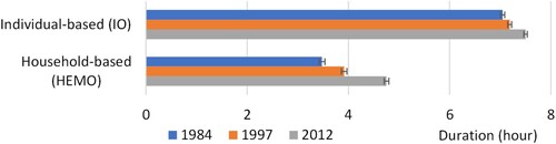
Figure 2 shows the transitions of the average IO and HEMO durations. The IO duration is longer than the HEMO duration for each year, and both the IO and HEMO durations increased. Notably, the HEMO duration increased by more than 1 h between 1984 and 2012. For a household with a single individual, the HEMO duration is equal to the IO duration; whereas, for a non-single household, the HEMO duration should be equal to or less than the IO durations of the household members by definition (Figure 1). Thus, the average HEMO duration is less than the average IO duration for each time period. To examine the reason for the increase in the HEMO duration, the HEMO durations for several household types were examined.

Figure 2. Transitions of average IO and HEMO durations. Bars indicate 95% confidence intervals for the averages.

Table 3 lists the transitions of the average HEMO durations by household size. The HEMO duration becomes longer for each household type. In addition, the HEMO duration of a smaller household is longer than that of a larger household in each year. This result is naturally explained by the fact that at least one-member in-home will create the household non-HEMO situation, and larger households tend to have non-HEMO situations. In addition, the difference in the HEMO durations between single-person households and two-person households is large, even though the size difference is just one person. These results imply that single-person households have a large impact on the HEMO duration.

Table 3. Transition of average HEMO duration by household size.

Household size	HEMO duration (hour)
	1984	1997	2012	2012–1984
1 person	6.11	6.38	6.56	0.45
2 people	3.15	3.23	3.94	0.79
3 people	2.77	3.04	3.63	0.86
4 people	2.69	3.03	3.71	1.02
5 people	1.66	2.24	2.93	1.27
6 people or more	0.38	0.70	1.17	0.79

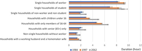
Figure 3 shows the average HEMO duration for each household composition. The HEMO durations of single-person households consisting of a worker or student are long, whereas that of single-person non-worker and non-student households is short. This reveals the impact of occupation on the HEMO duration. In addition, the duration of households with only members in the 16–64 age range is much longer than that of households with only seniors (65+), which indicates the age impact of the household members. The duration of households with a working husband and a homemaker wife is the shortest. Most household compositions reveal the increasing HEMO duration transition over the years. Particularly, single-person student households and households with children under 16 exhibit an increase of 2 h or more in the HEMO duration.

Figure 3. Transition of HEMO duration by household composition. Bars indicate 95% confidence interval for averages.

5.2. Spatial distribution of HEMO duration

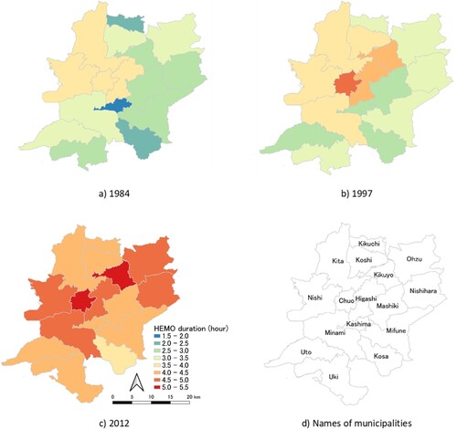
Figure 4 shows the average HEMO duration by municipality for the 3 years. Chuo-ward, which includes downtown Kumamoto, has the longest HEMO duration for each year. The duration increased greatly in Kikuyo and Kashima, whereas the duration in Kita-ward did not change much. The area with a longer HEMO duration spread toward the eastern side, including Kikuyo and Ohzu. The rapid urbanization in the eastern area partly explains this change. See Appendix B for the details of this analysis.

Figure 4. Average HEMO duration by municipality for 3 years.

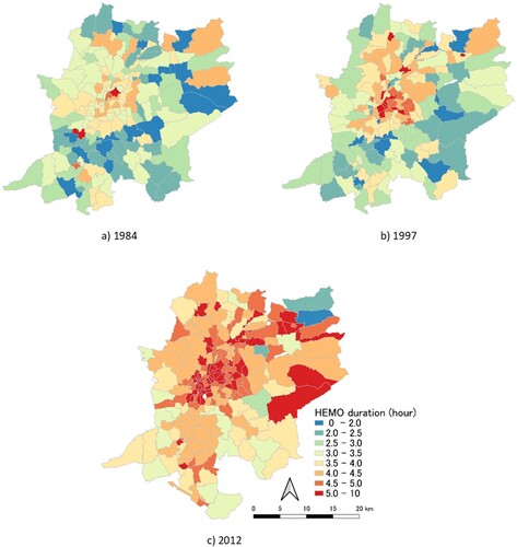
Figure 5 illustrates the spatiotemporal change in the HEMO duration on a detailed scale. It can be seen that there was a higher HEMO duration in the central area each year, as well as a gradual increase in the outer area. The southern part reveals a lower HEMO duration. Note that, although the number of TAZs is large (over 160), the large sample size of the PT surveys (Table 2) makes it possible to demonstrate the average HEMO duration by TAZ based on a sufficient sample size in most zones. The 5th and 95th percentiles of the household sample size in the TAZ are 75 and 380 for 1984, 22 and 408 for 1997, and 26 and 510 for 2012, respectively. In other words, 95% of the TAZ contained 75 or more household samples in 1984, for instance.

Figure 5. Average HEMO duration by traffic analysis zone for 3 years.

5.3. Econometric model results: Tobit model and time allocation model

Tables 4 and 5 list the estimation results from the Tobit and time allocation models, respectively. For each model type, three models were created with different variable sets: models A, B, and C. Model A was a base model; model B included the apartment-house rate as an additional variable; and model C included the apartment-house rate and interaction terms of household attribute variables and a dummy variable of the year. The apartment-house rate is the ratio of the number of apartment-house households to the total number of households in each TAZ, which represents the aggregated neighbourhood effect. The Akaike information criteria (AIC) of model B was smaller than that of model A, and the AIC of model C was the smallest for both the Tobit and time allocation models (Tables 4 and 5), which indicated that the inclusion of the apartment-house rate and interaction term was effective in improving the models. The AIC of the time allocation model was smaller than that of the Tobit model, indicating the better performance of the time allocation model.

Table 4. Estimation results of Tobit models.

	Model A: Base		Model B: with apartment-house rate		Model C: with apartment-house rate and interaction term
Variable	Parameter	t-value	Parameter	t-value	Parameter	t-value
Constant	4.82	68.40*	4.45	57.84*	4.41	46.36*
Household size	−3.04	−86.31*	−3.00	−84.97*	−2.80	−78.89*
Number of workers	2.30	75.10*	2.31	75.29*	2.19	71.01*
Number of children under 16	2.01	44.43*	1.98	43.72*	2.63	65.89*
Number of students	1.96	38.68*	1.92	37.79*	2.15	42.88*
Number of seniors (+65)	−1.07	−27.74*	−1.06	−27.50*	−1.29	−32.15*
Single-person households with worker dummy	3.38	60.91*	3.34	60.31*	3.32	59.43*
Single-person households with student dummy	3.03	23.36*	2.97	22.82*	3.46	21.54*
Households with children under 16 dummy	1.84	25.70*	1.83	25.61*	−0.03	−0.57
Households with seniors (65+) only dummy	−0.85	−12.24*	−0.82	−11.74*	−0.88	−8.98*
Households owning cars dummy	1.64	36.11*	1.69	37.08*	1.69	36.78*
Households with a working husband and a homemaker wife dummy	−1.76	−36.88*	−1.81	−37.70*	−1.87	−38.88*
1997 dummy	0.45	9.55*	0.37	7.81*	0.35	7.32*
2012 dummy	0.86	18.79*	0.71	15.17*	0.75	15.36*
Apartment-house rate			0.93	11.88*	0.93	11.83*
1984 dummy × Single-person households with student dummy					−1.35	−5.71*
2012 dummy × Households with seniors (65+) only dummy					0.22	2.21*
${\sigma }_1$	4.56	318.14*	4.56	318.17*	4.58	317.96
Sample size	84,732		84,732		84,732
Initial log likelihood for constant only model	−209,171		−209,171		−209,171
Final log likelihood	−188,313		−188,243		−188,225
McFadden's pseudo R^2	0.09972		0.10005		0.10014
AIC	376,652		376,513		376,483

*: p<0.01, AIC: Akaike information criteria.

Table 5. Estimation results of time allocation models.

	Model A: Base		Model B: with apartment-house rate		Model C: with apartment-house rate and interaction term
Variable	Parameter	t-value	Parameter	t-value	Parameter	t-value
Constant	−1.52	−92.11*	−1.57	−87.07*	−1.55	−84.98*
Household size	−0.69	−82.75*	−0.69	−81.89*	−0.69	−81.90*
Number of workers	0.56	77.48*	0.56	77.55*	0.56	77.55*
Number of children under 16	0.46	43.72*	0.46	43.26*	0.46	43.28*
Number of students	0.46	39.21*	0.46	38.65*	0.46	38.76*
Number of seniors (+65)	−0.24	−26.13*	−0.24	−25.97*	−0.24	−26.05*
Single-person households with worker dummy	0.72	56.09*	0.71	55.71*	0.71	55.45*
Single-person households with student dummy	0.70	23.63*	0.69	23.33*	0.79	21.60*
Households with children under 16 dummy	0.40	23.89*	0.40	23.88*	0.39	23.83*
Households with seniors (65+) only dummy	−0.16	−9.59*	−0.15	−9.31*	−0.19	−8.83*
Households owning cars dummy	0.33	31.00*	0.33	31.50*	0.33	30.94*
Households with a working husband and a homemaker wife dummy	−0.56	−49.91*	−0.57	−50.27*	−0.57	−50.39*
1997 dummy	0.12	11.06*	0.11	10.04*	0.10	9.27*
2012 dummy	0.21	19.84*	0.19	17.50*	0.18	15.65*
Apartment-house rate			0.12	6.65*	0.12	6.51*
1984 dummy × Single-person households with student dummy					−0.26	−4.81*
2012 dummy × Households with seniors (65+) only dummy					0.07	2.93*
${\sigma }_2$	1.04	332.27*	1.04	332.24*	1.04	332.20
Sample size	84,732		84,732		84,732
Initial log likelihood for constant only model	−120,176		−120,176		−120,176
Final log likelihood	−98,849		−98,827		−98,811
McFadden's pseudo R^2	0.17747		0.17765		0.17778
AIC	197,724		197,682		197,654

*: p<0.01, AIC: Akaike information criteria.

Most variables were statistically significant, which was partly due to the large sample size. Most variables had a reasonable sign. The estimated parameters revealed the various impacts of household attributes on the HEMO duration. In particular, single-person households with a worker or student had a larger HEMO duration. Owning a car had a positive and significant impact, with the household member with the car often taking trips and producing longer out-of-home times. The 1997 and 2012 dummies were positive and significant, and the 2012 dummy was larger; which showed the increased HEMO duration over the years. The apartment-house rate, which was positive and significant, indicated that areas with many apartment-buildings were neighbourhoods with longer HEMO durations. Appendix C examines the spatial autocorrelation of model C's residuals. It reveals a 5% autocorrelation in 1997 but no autocorrelation in 1984 and 2012, indicating the moderate performance of the estimated model. A future study will require the improvement of the 1997 model.

6. Discussion

The increase in the average HEMO duration (Figure 2) can mainly be explained by the increase in single-person households. The percentage of single-person households increased by more than 10% points between 1984 and 2012 and resulted in an average household size decrease (Table 2). The increase in the number of single-person households could be due to later marriages and people remaining unmarried, as well as an increase in the number of elderly people living alone. Therefore, the main reason for the increase in the HEMO duration was the increase in the number of small households, especially single-person households. This effect was reflected in the positive and significant parameters of single-person households with a worker or student dummy in Tables 4 and 5.

An increase in part-time working students partly explains the increase in the duration of single-person households with students (Figure 3). The effect was captured in the negative and significant parameters of the ‘1984 dummy × single-person households with student dummy’ in Tables 4 and 5. The increase in the number of active seniors increased the HEMO duration of households with seniors (65+) only (Figure 3). This effect was captured in the positive and significant parameters of the ‘2012 dummy × households with seniors (65+) only dummy’ in Tables 4 and 5. Increases in double-income and single-mother households partly explained the increase in the HEMO duration of households with children; these households may leave their children in childcare facility and childcare services during work, resulting in a longer HEMO duration.

After controlling the demographic variables, the HEMO duration was found to increase over time. The effect was captured in the estimates of the ‘1997 dummy’ and the ‘2012 dummy.’ They are both positive and significant, and the ‘2012 dummy’ is found to be larger than the ‘1997 dummy.’ The results indicate that the change in household demographic composition (e.g. increase in single households) is insufficient to explain the change in the total HEMO duration. In addition, it was found that the changes in travel behaviour for each household classification over time also change the HEMO duration.

The estimation results can lead to the following discussion on the effect of the variation in household members on the HEMO duration. The estimates of Tobit models are easily interpretable owing to their linear specification (Equation 1). Thus, we focus on the estimates of model C for the Tobit model. The estimate of −2.80 for ‘Household size’ indicates that the additional member to a household, on average, leads to a 2.8 h reduction in HEMO duration. If the additional member is a worker, the reduction will be 0.61 h due to the offsets of the estimates of ‘Household size’ and the ‘Number of workers’ ( = 2.80–2.19). Similarly, if the additional member is a senior, the reduction will be 4.09 h due to the addition of the estimates of ‘Household size’ and the ‘Number of workers’ ( = 2.8+1.29). A similar discussion can apply to other demographic attributes.

These findings enhanced the findings by Maruyama and Fukahori (2020), who analyzed the temporal profiles of the HEMO rate using the same data, through geographical visualization and statistical modelling. The temporal profile analysis demonstrated the HEMO change in the time-of-day, but the duration analysis neglected this change. The spatial variations of the temporal profiles of the HEMO rates cannot be demonstrated as simply as the spatial variations in the HEMO durations (Figures 4 and 5). Similarly, the statistical and econometric modelling of the temporal profiles of the HEMO rates is not as simple as that for the HEMO durations (Tables 4 and 5). Thus, the temporal profiles and duration analysis of the HEMO both have advantages and disadvantages and should complement each other.

To examine the cause of change in HEMO rate, Maruyama and Fukahori (2020) developed a decomposition method. Although their method is useful in demonstrating the change factor over the time-of-day, the method cannot provide the statistical significance of the factor. Furthermore, the method is limited because the decomposition should be based on a mutually exclusive and collectively exhaustive classification (e.g. a classification only by household size). The econometric models shown in this paper (i.e. Tobit and time allocation models) can handle several factors more flexibly than the decomposition method by Maruyama and Fukahori (2020).

The HEMO duration is a simple concept but not examined comprehensively in the existing literature, making it difficult to compare our results with other studies. Sekar et al. (2018) reported the decrease in the IO duration of the average Americans between 2003 and 2012, and Garikapati et al. (2016) implied the decrease in IO duration in younger millennials (born 1988–1994). Meanwhile, our results (Figure 2) indicate the increase in IO-duration between 1997 and 2012 in Kumamoto, Japan. The difference may be explained by the increasing share of active seniors in Kumamoto, but further examination is needed. We found no literature that provided changes in HEMO duration over time that is directly comparable to our results. However, calculating the HEMO duration can be straightforward using the household travel surveys or time-use survey data, and international comparison will be possible in future studies.

7. Conclusion

7.1. Key findings and contributions

This study explored the spatiotemporal change in the HEMO duration using the 1984, 1997 and 2012 Kumamoto PT surveys in Japan. The IO and HEMO durations increased over the years. Notably, the average HEMO duration increased by more than 1 h between 1984 and 2012. Increases in single-person households and active seniors could explain the increased HEMO duration. The length and transition of the HEMO duration varied across household types. The HEMO duration of single-person households with a worker or student was long, and that of households with a working husband and homemaker wife was short. The durations of single-person households with a student and households with children under 16 increased by more than 2 h over the 28 years. The HEMO durations increased in all municipalities, and those with rapid urbanization revealed a great increase. The downtown area revealed a longer HEMO duration and the area with a longer duration expanded to rural areas over the 28 years. Finally, Tobit and time allocation models successfully explained statistically the factors for the HEMO duration and its change.

This study's practical contribution and significance is the demonstration of HEMO duration map over time. The map can be produced easily using the existing household travel surveys, but no such map has been observed in the existing literature. This map can be a base for discussing several existing urban problems in practice. In addition, the proposal and implementation of the time-allocation modelling framework can be a theoretical contribution to the future HEMO studies in other countries.

7.2. Limitations and future perspectives

This subsection summarizes the limitations and future perspectives for this area of study. Maruyama and Fukahori (2020) discussed the issues with the used data, including the survey method differences for the 3 years, possible underreporting by mail- or web-based surveys, and effect of filtering samples, and expansion or weighting. They concluded that these issues would not be a severe problem. Thus, it was concluded that the current analysis using the same data would suffer little from the data issues.

This study used a time use model that is commonly used to explain an individual's time use for the HEMO analysis, but the individual and household time use allocations could follow a different mechanism. A group-based time duration model might provide a more plausible analysis framework in the future.

Applications of the HEMO duration may include the prevention of crimes such as burglaries, improved delivery services, and efficient survey visits (Maruyama & Fukahori, 2020). Specifically, the existing models explaining burglaries used demographic, socioeconomic, environmental, and other data as explanatory variables (Rummens, Hardyns, & Pauwels, 2017; Tseloni et al., 2004; Wilcox et al., 2007). The HEMO duration could be a promising new variable to improve the model. Furthermore, HEMO duration analysis may contribute to energy research by estimating the household power consumption. For example, Sekar et al. (2018) explored the effect of increase in the time spent at home over the years on the energy use in the U.S., and this HEMO duration analysis may enhance their analysis. In addition, this study used household travel surveys to calculate the duration, but time use surveys are another option. The comparison or integration of these data can be included in future work.

The literature on time use modelling demonstrated that time use fluctuates over days (Spissu et al., 2009; Watanabe, Chikaraishi, & Maruyama, 2021). Thus, the HEMO duration will also fluctuate. The traditional household travel survey with cross section data cannot handle such fluctuations, but new data such as the day-to-day energy consumption collected by a smart metre may be used to infer the fluctuations in the HEMO duration in future work.

In 2020–2022, the stay-at-home orders and policies to restrict activities in response to the COVID-19 pandemic would have reduced HEMO durations in cities worldwide. Telework and remote meetings (Budnitz, Tranos, & Chapman, 2020; Kim, Choo, & Mokhtarian, 2015; Shabanpour, Golshani, Tayarani, Auld, & Mohammadian, 2018b; Stiles & Smart, 2021) would have greatly increased and reduced the HEMO duration. Investigating such effects with additional survey data (Arroyo, Mars, & Ruiz, 2021; J. Liu et al., 2021; Shamshiripour, Rahimi, Shabanpour, & Mohammadian, 2020; Yilmazkuday, 2021) and modelling out-of-home and in-home activity participation (Fatmi, Thirkell, & Hossain, 2021; Hossain, Haque, & Fatmi, 2022) will be included in our future work.

Acknowledgments

This research was funded by JSPS KAKENHI, grant number JP19K21997. The Kumamoto prefectural government provided the household travel survey data. Yoshihiro Sato supported us in the preparation of the data. Tatsuya Fukahori supported us in the calculation of the HEMO. Hajime Watanabe supported the statistical modelling. We would like to express our gratitude for this support. Any remaining errors are the authors’ responsibility.

Data availability statement

The Kumamoto Person Trip survey data presented in this study were supplied by Kumamoto prefectural government under license and so cannot be made freely available. Requests for access to these data should be made to Kumamoto prefectural government.

Disclosure statement

No potential conflict of interest was reported by the author(s).

Additional information

Funding

This work was supported by JSPS: [Grant Number JP19K21997].

References

- Akar, G., Clifton, K. J., & Doherty, S. T. (2011). Discretionary activity location choice: In-home or out-of-home? Transportation, 38(1), 101–122. doi:10.1007/s11116-010-9293-x
- Anderson, B., & Torriti, J. (2018). Explaining shifts in UK electricity demand using time use data from 1974 to 2014. Energy Policy, 123, 544–557. doi:10.1016/j.enpol.2018.09.025
- Aragon, V., Gauthier, S., Warren, P., James, P. A. B., & Anderson, B. (2019). Developing English domestic occupancy profiles. Building Research & Information, 47(4), 375–393. doi:10.1080/09613218.2017.1399719
- Arroyo, R., Mars, L., & Ruiz, T. (2021). Activity participation and wellbeing during the COVID-19 lockdown in Spain. International Journal of Urban Sciences, 25(3), 386–415. doi:10.1080/12265934.2021.1925144
- Barthelmes, V. M., Li, R., Andersen, R. K., Bahnfleth, W., Corgnati, S. P., & Rode, C. (2018). Profiling occupant behaviour in Danish dwellings using time use survey data. Energy and Buildings, 177, 329–340. doi:10.1016/j.enbuild.2018.07.044
- Bernardo, C., Paleti, R., Hoklas, M., & Bhat, C. (2015). An empirical investigation into the time-use and activity patterns of dual-earner couples with and without young children. Transportation Research Part A: Policy and Practice, 76, 71–91. doi:10.1016/j.tra.2014.12.006
- Bhat, C. R., Goulias, K. G., Pendyala, R. M., Paleti, R., Sidharthan, R., Schmitt, L., & Hu, H. H. (2013). A household-level activity pattern generation model with an application for Southern California. Transportation, 40(5), 1063–1086. doi:10.1007/s11116-013-9452-y
- Bhat, C. R., & Misra, R. (1999). Discretionary activity time allocation of individuals between in-home and out-of-home and between weekdays and weekends. Transportation, 26(2), 193–209. doi:10.1023/A:1005192230485
- Budnitz, H., Tranos, E., & Chapman, L. (2020). Telecommuting and other trips: An English case study. Journal of Transport Geography, 85, 102713. doi:10.1016/j.jtrangeo.2020.102713
- Buldeo Rai, H., Verlinde, S., & Macharis, C. (2021). Unlocking the failed delivery problem? Opportunities and challenges for smart locks from a consumer perspective. Research in Transportation Economics, 87, 100753. doi:10.1016/j.retrec.2019.100753
- Calastri, C., Hess, S., Daly, A., & Carrasco, J. A. (2017). Does the social context help with understanding and predicting the choice of activity type and duration? An application of the Multiple Discrete-Continuous Nested Extreme Value model to activity diary data. Transportation Research Part A: Policy and Practice, 104, 1–20. doi:10.1016/j.tra.2017.07.003
- Calvo, F., Eboli, L., Forciniti, C., & Mazzulla, G. (2019). Factors influencing trip generation on metro system in Madrid (Spain). Transportation Research Part D: Transport and Environment, 67, 156–172. doi:10.1016/j.trd.2018.11.021
- Cazabet, R., Jensen, P., & Borgnat, P. (2018). Tracking the evolution of temporal patterns of usage in bicycle-sharing systems using nonnegative matrix factorization on multiple sliding windows. International Journal of Urban Sciences, 22(2), 147–161. doi:10.1080/12265934.2017.1336468
- Chen, L., & Jiang, S. (2021). Spatiotemporal polyrhythm characteristics of public bicycle mobility in urban chronotopes context. ISPRS International Journal of Geo-Information, 11(1), 6. doi:10.3390/ijgi11010006
- De Lauretis, S., Ghersi, F., & Cayla, J. M. (2017). Energy consumption and activity patterns: An analysis extended to total time and energy use for French households. Applied Energy, 206, 634–648. doi:10.1016/j.apenergy.2017.08.180
- Deville, P., Linard, C., Martin, S., Gilbert, M., Stevens, F. R., Gaughan, A. E., … Tatem, A. J. (2014). Dynamic population mapping using mobile phone data. Proceedings of the National Academy of Sciences of the United States of America, 111(45), 15888–15893. doi:10.1073/pnas.1408439111
- Diao, L., Sun, Y., Chen, Z., & Chen, J. (2017). Modeling energy consumption in residential buildings: A bottom-up analysis based on occupant behavior pattern clustering and stochastic simulation. Energy and Buildings, 147, 47–66. doi:10.1016/j.enbuild.2017.04.072
- Enam, A., & Konduri, K. C. (2018). Time allocation behavior of twentieth-century American generations: GI generation, silent generation, baby boomers, generation X, and millennials. Transportation Research Record: Journal of the Transportation Research Board, 2672(49), 69–80. doi:10.1177/0361198118794710
- Enam, A., Konduri, K. C., Eluru, N., & Ravulaparthy, S. (2018). Relationship between well-being and daily time use of elderly: Evidence from the disabilities and use of time survey. Transportation, 45(6), 1783–1810. doi:10.1007/S11116-017-9821-Z/TABLES/4
- Fatmi, M. R., Thirkell, C., & Hossain, M. S. (2021). COVID-19 and travel: How our out-of-home travel activity, in-home activity, and long-distance travel have changed. Transportation Research Interdisciplinary Perspectives, 10, 100350. doi:10.1016/J.TRIP.2021.100350
- Feng, J., Chuai, X., Lu, Y., Guo, X., & Yuan, Y. (2020). Who will do more? The pattern of daily out-of-home activity participation in elderly co-residence households in urban China. Cities, 98, 102586. doi:10.1016/j.cities.2019.102586
- Fu, X. (2020). How do out-of-home workers spend their daily time? An empirical comparison across five cities in China. Travel Behaviour and Society, 21, 203–213. doi:10.1016/j.tbs.2020.07.001
- Fukahori, T., & Maruyama, T. (2021). Evolutions of households with every member out-of-home across Japanese cities from 1987 to 2015. Computers, Environment and Urban Systems, 89, 101683. doi:10.1016/j.compenvurbsys.2021.101683
- Garikapati, V. M., Pendyala, R. M., Morris, E. A., Mokhtarian, P. L., & McDonald, N. (2016). Activity patterns, time use, and travel of millennials: A generation in transition? Transport Reviews, 36(5), 558–584. doi:10.1080/01441647.2016.1197337
- Hossain, M. (2020). Sharing economy: A comprehensive literature review. International Journal of Hospitality Management, 87, 102470. doi:10.1016/J.IJHM.2020.102470
- Hossain, M. S., Haque, K., & Fatmi, M. R. (2022). COVID-19: Modeling out-of-home and in-home activity participation during the pandemic. Transportation Research Record: Journal of the Transportation Research Board, 036119812110677. doi:10.1177/03611981211067790
- Kelobonye, K., McCarney, G., Xia, J. (Cecilia), Swapan, M. S. H., Mao, F., & Zhou, H. (2019). Relative accessibility analysis for key land uses: A spatial equity perspective. Journal of Transport Geography, 75, 82–93. doi:10.1016/J.JTRANGEO.2019.01.015
- Kelobonye, K., Zhou, H., McCarney, G., & Xia, J. (Cecilia) (2020). Measuring the accessibility and spatial equity of urban services under competition using the cumulative opportunities measure. Journal of Transport Geography, 85, 102706. doi:10.1016/J.JTRANGEO.2020.102706
- Kim, K., Han, S.-L., Jang, Y.-Y., & Shin, Y.-C. (2020). The effects of the antecedents of “buy-online-pick-up-in-store” service on consumer’s BOPIS choice behaviour. Sustainability, 12(23), 9989. doi:10.3390/su12239989
- Kim, S. N., Choo, S., & Mokhtarian, P. L. (2015). Home-based telecommuting and intra-household interactions in work and non-work travel: A seemingly unrelated censored regression approach. Transportation Research Part A: Policy and Practice, 80, 197–214. doi:10.1016/j.tra.2015.07.018
- Kim, W., & Wang, X. C. (2022). The adoption of alternative delivery locations in New York City: Who and how far? Transportation Research Part A: Policy and Practice, 158, 127–140. doi:10.1016/J.TRA.2022.02.006
- Kitamura, R. (1984). A model of daily time allocation to discretionary out-of-home activities and trips. Transportation Research Part B, 18(3), 255–266. doi:10.1016/0191-2615(84)90036-5
- Kleiminger, W., Mattern, F., & Santini, S. (2014). Predicting household occupancy for smart heating control: A comparative performance analysis of state-of-the-art approaches. Energy and Buildings, 85, 493–505. doi:10.1016/j.enbuild.2014.09.046
- KMTC. (2016). Report on Kumamoto Metropolitan Area Urban Transportation Master Plan. Kumamoto Metropolitan Area Transportation Council.
- Kuhnimhof, T., Armoogum, J., Buehler, R., Dargay, J., Denstadli, J. M., & Yamamoto, T. (2012). Men shape a downward trend in car use among young adults—evidence from six industrialized countries. Transport Reviews, 32(6), 761–779. doi:10.1080/01441647.2012.736426
- Lai, M., Cai, X., & Hu, Q. (2021). Market design for commute-driven private parking lot sharing. Transportation Research Part C: Emerging Technologies, 124, 102915. doi:10.1016/J.TRC.2020.102915
- Lai, X., Lam, W. H. K., Su, J., & Fu, H. (2019). Modelling intra-household interactions in time-use and activity patterns of retired and dual-earner couples. Transportation Research Part A: Policy and Practice, 126, 172–194. doi:10.1016/j.tra.2019.05.007
- Liu, J., Gross, J., & Ha, J. (2021). Is travel behaviour an equity issue? Using GPS location data to assess the effects of income and supermarket availability on travel reduction during the COVID-19 pandemic. International Journal of Urban Sciences, 25(3), 366–385. doi:10.1080/12265934.2021.1952890
- Liu, S., Yamamoto, T., Yao, E., & Nakamura, T. (2021). Examining public transport usage by older adults with smart card data: A longitudinal study in Japan. Journal of Transport Geography, 93, 103046. doi:10.1016/j.jtrangeo.2021.103046
- Maruyama, T., & Fukahori, T. (2020). Households with every member out-of-home (HEMO): Comparison using the 1984, 1997, and 2012 household travel surveys in Kumamoto, Japan. Journal of Transport Geography, 82, 102632. doi:10.1016/J.JTRANGEO.2019.102632
- Meloni, I., Guala, L., & Loddo, A. (2004). Time allocation to discretionary in-home, out-of-home activities and to trips. Transportation, 31(1), 69–96. doi:10.1023/B:PORT.0000007228.44861.ae
- Miwa, T., Yamamoto, T., & Morikawa, T. (2009). Inter-temporal and inter-regional comparative analyses on household shared time. Journal of the City Planning Institute of Japan, 44(3), 745–750. doi:10.11361/journalcpij.44.3.745
- Morris, E. A. (2015). Should we all just stay home? Travel, out-of-home activities, and life satisfaction. Transportation Research Part A: Policy and Practice, 78, 519–536. doi:10.1016/j.tra.2015.06.009
- Rovira, Y. L., Imani, A. F., Sivakumar, A., & Pawlak, J. (2022). Do in-home and virtual activities impact out-of-home activity participation? Investigating end-user activity behaviour and time use for residential energy applications. Energy and Buildings, 257, 111764. doi:10.1016/J.ENBUILD.2021.111764
- Rummens, A., Hardyns, W., & Pauwels, L. (2017). The use of predictive analysis in spatiotemporal crime forecasting: Building and testing a model in an urban context. Applied Geography, 86, 255–261. doi:10.1016/j.apgeog.2017.06.011
- Sekar, A., Williams, E., & Chen, R. (2018). Changes in time use and their effect on energy consumption in the United States. Joule, 2(3), 521–536. doi:10.1016/j.joule.2018.01.003
- Shabanpour, R., Golshani, N., Fasihozaman Langerudi, M., & Mohammadian, A. (Kouros). (2018a). Planning in-home activities in the ADAPTS activity-based model: A joint model of activity type and duration. International Journal of Urban Sciences, 22(2), 236–254. doi:10.1080/12265934.2017.1313707
- Shabanpour, R., Golshani, N., Tayarani, M., Auld, J., & Mohammadian, A. (Kouros) (2018b). Analysis of telecommuting behavior and impacts on travel demand and the environment. Transportation Research Part D: Transport and Environment, 62, 563–576. doi:10.1016/J.TRD.2018.04.003
- Shamshiripour, A., Rahimi, E., Shabanpour, R., & Mohammadian, A. K. (2020). How is COVID-19 reshaping activity-travel behavior? Evidence from a comprehensive survey in Chicago. Transportation Research Interdisciplinary Perspectives, 7, 100216. doi:10.1016/J.TRIP.2020.100216
- Shao, C., Yang, H., Zhang, Y., & Ke, J. (2016). A simple reservation and allocation model of shared parking lots. Transportation Research Part C: Emerging Technologies, 71, 303–312. doi:10.1016/J.TRC.2016.08.010
- Shi, Z., Pun-Cheng, L. S. C., Liu, X., Lai, J., Tong, C., Zhang, A., … Shi, W. (2020). Analysis of the temporal characteristics of the elderly traveling by bus using smart card data. ISPRS International Journal of Geo-Information, 9(12), 751. doi:10.3390/ijgi9120751
- Spinney, J. E. L., Newbold, K. B., Scott, D. M., Vrkljan, B., & Grenier, A. (2020). The impact of driving status on out-of-home and social activity engagement among older Canadians. Journal of Transport Geography, 85, 102698. doi:10.1016/j.jtrangeo.2020.102698
- Spissu, E., Pinjari, A. R., Bhat, C. R., Pendyala, R. M., & Axhausen, K. W. (2009). An analysis of weekly out-of-home discretionary activity participation and time-use behavior. Transportation, 36(5), 483–510. doi:10.1007/s11116-009-9200-5
- Srinivasan, S., & Bhat, C. R. (2005). Modeling household interactions in daily in-home and out-of-home maintenance activity participation. Transportation, 32(5), 523–544. doi:10.1007/s11116-005-5329-z
- Stiles, J., & Smart, M. J. (2021). Working at home and elsewhere: Daily work location, telework, and travel among United States knowledge workers. Transportation, 48(5), 2461–2491. doi:10.1007/s11116-020-10136-6
- Stopher, P. R., & Greaves, S. P. (2007). Household travel surveys: Where are we going? Transportation Research Part A: Policy and Practice, 41(5), 367–381. doi:10.1016/j.tra.2006.09.005
- Tan, S. Y., Jacoby, M., Saha, H., Florita, A., Henze, G., & Sarkar, S. (2022). Multimodal sensor fusion framework for residential building occupancy detection. Energy and Buildings, 258, 111828. doi:10.1016/j.enbuild.2021.111828
- Tobin, J. (1958). Estimation of relationships for limited dependent variables. Econometrica, 26(1), 24–36. doi:10.2307/1907382
- Tseloni, A., Wittebrood, K., Farrell, G., & Pease, K. (2004). Burglary victimization in England and Wales, the United States and the Netherlands: A cross-national comparative test of routine activities and lifestyle theories. British Journal of Criminology, 44(1), 66–91. doi:10.1093/bjc/44.1.66
- Van Duin, J. H. R., De Goffau, W., Wiegmans, B., Tavasszy, L. A., & Saes, M. (2016). Improving home delivery efficiency by using principles of address intelligence for B2C deliveries. Transportation Research Procedia, 12, 14–25. doi:10.1016/j.trpro.2016.02.006
- Van Duin, J. H. R., Wiegmans, B. W., Van Arem, B., & Van Amstel, Y. (2020). From home delivery to parcel lockers: A case study in Amsterdam. Transportation Research Procedia, 46, 37–44. doi:10.1016/J.TRPRO.2020.03.161
- Wang, H., Huang, H., Ni, X., & Zeng, W. (2019). Revealing spatial-temporal characteristics and patterns of urban travel: A large-scale analysis and visualization study with taxi GPS data. ISPRS International Journal of Geo-Information, 8(6), 257. doi:10.3390/ijgi8060257
- Washington, S., Karlaftis, M., Mannering, F., & Anastasopoulos, P. (2020). Statistical and econometric methods for transportation data analysis. Chapman and Hall/CRC. doi:10.1201/9780429244018.
- Watanabe, H., Chikaraishi, M., & Maruyama, T. (2021). How different are daily fluctuations and weekly rhythms in time-use behavior across urban settings? A case in two Japanese cities. Travel Behaviour and Society, 22, 146–154. doi:10.1016/j.tbs.2020.09.004
- Wilcox, P., Madensen, T. D., & Tillyer, M. S. (2007). Guardianship in context: Implications for burglary victimization risk and prevention. Criminology; An interdisciplinary Journal, 45(4), 771–803. doi:10.1111/j.1745-9125.2007.00094.x
- Xu, S. X., Cheng, M., Kong, X. T. R., Yang, H., & Huang, G. Q. (2016). Private parking slot sharing. Transportation Research Part B: Methodological, 93, 596–617. doi:10.1016/J.TRB.2016.08.017
- Yamamoto, T., & Kitamura, R. (1999). An analysis of time allocation to in-home and out-of-home discretionary activities across working days and non-working days. Transportation, 26(2), 231–250. doi:10.1023/a:1005167311075
- Yamamoto, T., Miwa, D., & Morikawa, T. (2009). Analysis of household joint activity engagement using person trip survey data and time use and leisure activity survey data. Proceedings of 39th JSCE IP Conference.
- Yilmazkuday, H. (2021). Unequal welfare costs of staying at home across socioeconomic and demographic groups. International Journal of Urban Sciences, 25(3), 347–365. doi:10.1080/12265934.2021.1951822
- Zhang, C., & Chen, J. (2021). Evaluation of residential parking spots sharing effects based on practical experience. Journal of Advanced Transportation, 2021, 1–13. doi:10.1155/2021/6222813
- Zhang, F., Liu, W., Wang, X., & Yang, H. (2020). Parking sharing problem with spatially distributed parking supplies. Transportation Research Part C: Emerging Technologies, 117, 102676. doi:10.1016/J.TRC.2020.102676
- Zhang, W., Ji, C., Yu, H., Zhao, Y., & Chai, Y. (2021). Interpersonal and intrapersonal variabilities in daily activity-travel patterns: A networked spatiotemporal analysis. ISPRS International Journal of Geo-Information, 10(3), 148. doi:10.3390/ijgi10030148