Rapid generation of human femur models based on morphological parameters and mesh deformation

ABSTRACT

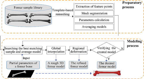
In this paper a new method for generating human femur models was presented, which combined parametric technology and deformation technology. The main target of our proposed method was to quickly generate a three-dimensional model which would best suit the patient's femur bone, even if a part of the bone was damaged or only partial data about the bone shape is available. First, all femur sample models were remeshed so as to have the same topology as the template, which enabled them to achieve compatible mesh segmentation quickly. Then, complete morphological parameters of all femur samples were calculated effectively and thereby a parameter set was got, which served as both reference and a constraint for generating new femur models. Next, according to partial known parameters, the best matching sample and the average model were selected to create a rough femur model through global interpolation. Finally, the rough model was further deformed locally to modify details until the desired femur model was obtained. Experimental results showed that the proposed method could efficiently generate anatomically suitable femur models, of which both the parameter error and the shape error were clinically acceptable.

KEYWORDS:

• Model generation
• femur parameter measurement
• mesh segmentation
• mesh deformation

Introduction

In orthopaedic surgery, three-dimensional models of human bones are of great significance for preoperative planning, intraoperative execution and post-operative evaluation, most notably for designing customized implants and fixators. However, generating a surface model from the given data such as computed tomography (CT) images is tedious, time consuming and error prone, especially in the cases where the medical images are incomplete or of poor quality. Furthermore, orthopaedic patients often have some degree of skeleton damage or deformity due to osteoporosis, arthritis, tumour, fracture, etc. Therefore, it is difficult to generate anatomically suitable 3D models. Frequently the bone model is created by approximation of its shape, which considerably reduces model quality and increases the risk of surgery. Thus, an effective method for the generation of bone models which can meet the clinical need is highly desirable.

As for the modelling method, many techniques have been developed in the past two decades. In particular, parametric technology and deformation technology have received extensive attention. Parametric modelling allows the designer to control a shape by assigning numerical values to several parameters such as length, width and height, because these parameters have a procedural relationship with the data for a shape [1–3]. However, due to the inherent complexity of the human bone's anatomical structures, it is hard to define the bone shape with several simple parameters. Utilizing the morphological parameters to represent the bone geometry is a good choice. However, the morphological measurement is not easy. Taking femur bone as an example, morphological data was previously measured from cadaveric specimens manually or by a radiographic method [4–6]. Both methods are basically a 2D assessment, which may not accurately reflect the complex 3D morphology of the femur. Another measurement method is to calculate the parameters on 3D femur models, which are reconstructed from clinical CT images by reverse engineering technique. However, the majority of the related documents are limited to the morphology of proximal femur, and cannot offer enough parameters to completely describe the femur shape [7–9]. In this paper, we calculated complete morphological parameters about the whole femur bone based on a semantic-oriented mesh segmentation.

Deformation technology has been widely used in many areas such as modelling the geometry of face or body [10–12], but so far few documents have been reported on application of the technology in generating human bone models. The reasons mainly lie in the difficulty in maintaining the anatomical characteristics of the deformed bone model. Deformation in facial expressions or body poses allows relatively large scale, as long as the vision can endure. But human bone has its specific anatomical characteristics. Even if the deformed bone model is visually acceptable, it may be unrealistic for not satisfying the anatomical characteristics. In the clinical study of orthopaedic surgery, a few documents have been reported in generating new bone models by applying mesh deformation technology [13–15]. In these methods, local region is deformed independently with the change of a certain parameter; meanwhile, other regions and parameters remain unchanged. However, they have not considered the anatomical characteristics of the deformed bone models. Numerous morphological studies on human bones have proved that morphological parameters are correlative and interactive. So, in our opinion, the method of deforming local region independently is only suitable for slight adjustment in the parameter. If major adjustment is needed, the model must be overall deformed to maintain the correlation between parameters.

In this paper a new method for the generation of human femur models is presented, which combined parametric technology and deformation technology. With a template-related strategy, we calculated complete morphological parameters effectively for all femur samples and thereby got a parameter set, which could serve as both reference and a constraint for generating new femur models. Our goal was to deform the existing sample model into the altered shape which best suits the patient's femur bone even if a part of the bone was damaged or only a single X-ray image is available. For this purpose, we first applied global interpolation of suitable sample to obtain a rough femur model and then refined it through local deformation. The generated femur model incorporated the detailed information of a particular patient while leveraging the standardized geometry of the average model built from femur samples. The patient data herein was described as some morphological parameters which could be acquired from medical images such as CT or X-ray.

Materials and methods

The presented method was generally divided into the preparatory process and the modelling process, as illustrated in Figure 1. By using a template-related strategy, complete morphological parameters of all femur sample models were calculated effectively based on mesh segmentation. Then, according to partial known parameters, the best matching sample and average model were selected to perform global interpolation. As a result, a rough femur model was created, whose certain regions would be further deformed locally to modify details until the desired femur model was obtained.

Figure 1. Schematic diagram of the proposed method. Starting from a set of femur sample models, the desired 3D modem which best suited the parent's femur bone could be generated even if a part of the bone was damaged or only partial data about the bone shape was available.

The preparatory process

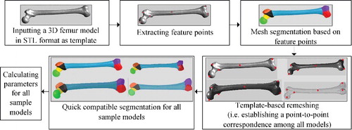
In this stage, parameter measurement was performed for each femur sample based on mesh segmentation. Considering the inefficiency in processing each sample separately, we selected a well-processed femur model as template, for guiding other sample models to achieve quick compatible segmentation (i.e. identically segmenting objects that are visually similar). However, the premise of this strategy was that all other sample models should be remeshed to have the same topology as the template model. Both mesh segmentation and parameter measurement relied heavily on feature points, which could be a prominent point on the condyle, or a boundary point between two different regions. Therefore, extraction of feature points was carried out in the first step. Figure 2 illustrated the flow chart of the preparatory process, which consisted of the following steps:

• Step 1: Feature points on the template model were extracted.

• Step 2: The template model was segmented into several anatomical regions based on feature points.

• Step 3: All other sample models were remeshed to have the same topology as the template mesh model.

• Step 4: Quick compatible segmentation was performed for all sample models.

• Step 5: Parameters for all sample models were calculated.

Figure 2. Flow chart for the preparatory process.

Feature points extraction and mesh segmentation

According to demands for mesh segmentation and parameters measurement, the feature points could be divided into three categories: (1) centre point, (2) salient point and (3) boundary point.

It was relatively simple to locate the centre point of the model: First, the 3D coordinates of all mesh vertices were averaged to obtain a spatial location, which was often not on the model surface. Then the nearest mesh vertex to the spatial location was selected as the centre point. For the femur model, the centre point positioned in this way always fell into the region of femoral shaft because this region occupied the largest volume of the model.

Salient points were the local extreme points of the model. Intuitively, they should reside on tips of prominent components of a given model. Salient points could be detected by the property of having local maximum of the sum of the geodesic distance to all other points of the mesh [16,17]. To reduce the computational cost, we replaced the sum distance with the distance just to the centre point, which was solved by Dijkstra's algorithm based on edge length, i.e. following the increasing order of the path length, the shortest path from each vertex to the centre point was computed in sequence.

However, the points extracted with the aforementioned property may contain some other points that were not salient points, due to small noise. Therefore, filtering was necessary which often required prior knowledge or a user-defined threshold. In our method, the detected salient points were filtered by local depth, which was defined as the largest height difference between a given vertex and its neighbour vertices on a 3D model [18]. For a given vertex, if its local depth was negative, and the smaller the value was, the more likely it is located at the position of convex. Thus this characteristic could be used as another condition for detecting salient points. Meanwhile, conversely, if the local depth was positive and the larger the value was, the more likely the vertex is located at the position of concave, and then it could be detected as the boundary point between two regions.

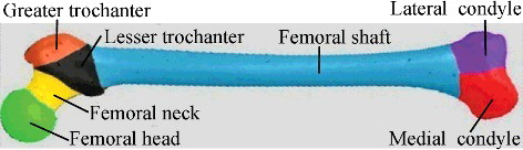
As a medical model, each part of the femur had specific medical semantics, only geodesic distance and local depth were not sufficient for accurately extracting all feature points. So, identifying feature points in some parts also required moderate manual interactions based on prior knowledge about the bone anatomy. To illustrate it, the salient point of greater trochanter was taken as an example: greater trochanter was an upward bulge which is located at the lateral border between femoral neck and body. As shown in Figure 3, the mesh surface had very poor smoothness and more than one candidate salient point (marked with small balls in Figure 3) was extracted only based on geometrical properties. According to the anatomical characteristics of the femur, greater trochanter point should be the vertex which was the farthest in this region to the centre of the femoral shaft, namely the upper edge point of the greater trochanter region. Therefore, among all candidate salient points in this region, the vertex with the largest distance to the centre point was selected as the greater trochanter point.

Figure 3. Schematic diagram of searching for greater trochanter point.

Figures 4 and 5 show all the three kinds of feature points on the femur model. Based on these feature points, mesh segmentation could be performed. Segmentation was helpful for calculating regional parameters of the model. Furthermore, it laid the foundation for later regional deformation. Aiming at partitioning a 3D bone model into several anatomical regions, we adopted marker-controlled fast marching watershed algorithm [19,20]. Different from existing methods, we used aforementioned salient points and centre point as markers. Then based on geodesic distance value, the marker points acted as seeds to perform region growing, which was terminated by boundary points. Figure 6 shows the segmentation result of the femur model. Similarly, for the sake of obtaining the desired segmentation result to be consistent with the specific medical semantics of the femur, moderate manual interactions got involved during the process.

Figure 4. Centre point and salient points of femur model.

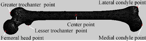
Figure 5. Boundary points of femur model.

Figure 6. Segmentation result of femur model.

Template-based remeshing and compatible segmentation

In this step, all sample models were remeshed to have the same topology as the template model. Such remeshing could also form the basis for calculating the average model, which acted as the benchmark for later overall deformation. The key of remeshing was to establish a point-to-point correspondence between models. To do so, we applied a template-based non-rigid registration technique. Unlike previous approaches [11,12,21], our registration technique was based on Laplacian editing [22], as all femur models were in similar shape, just varying in structural details.

The main idea of our method was to keep the Laplacian coordinates (represented by the difference of a vertex position from the centroid of its neighbours) of all mesh vertices unchanged, meanwhile keeping constraint points unchanged. Using Laplacian editing, the source model could be deformed smoothly toward the target model while preserving the geometric details as much as possible. To guarantee the correspondence between all pairs of feature points on the two given models, all feature points were used as constraint points during Laplacian deformation. In some relatively smooth areas such as femoral shaft region, feature points were not sufficient to ensure the registration quality, thus a few randomly selected vertices were added as constraint points.

As shown in Figure 7, A, B, C, D and E are all femur mesh models. Taking A as the template model and B as the target model, the specific model registration method was described as follows: First, utilizing the iterative closest point algorithm [23], i.e. by estimating the optimal rotation and translation, model A was positioned to be in best alignment with model B. Then, Laplacian surface editing on model A in reference with model B was performed. After several deformation iterations, new triangle mesh model B_l was generated from A. On one hand, B_l was created referring to the geometric characteristics of target B, B_l could approximate the shape of B and therefore we used B_l instead of B in the subsequent procedure. On the other hand, because B_l originated from template A, B_l was exactly equal to A in topology. In the same way, new models of C_l, D_l and E_l were the remeshed results corresponding to target models of C, D and E, respectively, and they all had the same topology as the template model A.

Figure 7. Generating consistent mesh: all the other femur models were remeshed to have the same topology as template A.

Once a point-to-point correspondence was established between template model and non-template models by remeshing, it was easy to transfer the segmentation information of template model to non-template models, thus achieving compatible segmentation. In this case, the transfer was simple: as the vertices in each model were in correspondence, the segmented region number of each vertex could be directly copied. The segmentation result obtained in this way was sometimes not very precise, but doing so was quick and easy. In fact, it was not necessary to partition the bone model that precisely, because the medical definition for the border between regions of the bone was not absolute.

Parameter calculation

After mesh segmentation, regions including femoral head, shaft and neck could be fitted by proper primitives, as shown in Figure 8, and then relevant parameters were calculated in combination with feature points. The remaining portions including femoral condyle, greater trochanter and lesser trochanter constituted of irregular surfaces with no specific geometric characteristics, thus more feature points within these regions were utilized to improve the measurement. That way, a series of morphological parameters were measured, some of which are listed in Table 1. These parameters beared great guiding significance for orthopaedic surgery and prostheses design [24–26].

Figure 8. Surface fitting results of some regions.

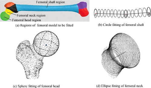
Table 1. Main morphological parameters of femur model.

Parameter type	Parameter name and description
Regional parameter	Femoral head diameter
	Femoral neck length
	Neck isthmus diameter
	Femoral shaft length
	Shaft isthmus diameter
	Shaft curvature radius
	Gaussian curvature at greater trochanter point
	Gaussian curvature at lesser trochanter point
	Anterior–posterior diameter of lateral condyle
	Anterior–posterior diameter of medial condyle
	Width of lateral condyle
	Width of medial condyle
Inter-regional parameter	Condyle width(width of whole condyle)
	Head–shaft offset (distance from head centre to shaft axis)
	Distance from head centre to lesser trochanter plane
	Distance from greater trochanter point to lesser trochanter point
	Neck–shaft angle
Key parameter	Femur length

In order to facilitate the subsequent deformation process, these parameters were classified into regional parameter, inter-regional parameter and key parameter. The regional parameter was used to describe the local feature of a region. For example, regional feature of the femoral condyle could be described by anterior–posterior diameter, width and so on. The inter-regional parameter was associated with more than one region, reflecting the global feature of the model. For example, neck-shaft angle reflected the structural relationship between the regions of femoral head, neck and shaft. In particular, among these parameters, femur length was regarded as key parameter because it involved multiple areas and was closely related to the body height (accounting for about 27% of body height).

As mentioned earlier, morphological parameters of femur bone were correlative and interactive. For example, head–shaft offset was negatively correlated with neck–shaft angle, but was positively correlated with femoral head diameter. As for femur length, it had a strong positive correlation with most linear parameters such as femoral neck length, head diameter and condyle width [14,27–30]. Therefore, when generating new femur models, the correlation between the parameters should be taken into account. The inter-regional parameter, in particular, was not suitable to be changed through separately deforming some local region. In later modelling process, inter-regional parameters had priority to regional parameters to be satisfied, respectively, by global deformation and local deformation.

Generating the desired femur model according to partial known parameters

After preparatory process, according to partial known parameters, a rough femur model could be created through global interpolation. Then certain regions were further deformed independently to modify details. Finally, to verify the validity of the generated model, not only the parameter error but also the shape error was measured.

Overall deformation

The purpose of overall deformation was to obtain a rough model from existing sample models by adopting interpolation method, based on known key parameter or inter-regional parameters. Since all femur samples were in full correspondence after remeshing, a new femur model could be generated by simply taking linear combinations of the coordinates of matching vertices between any two samples. And by changing the interpolation ratio, the shape of the new model would be changed correspondingly. Figure 9 shows a series of new femur models which were generated by linear interpolation between two arbitrary samples. These new models had the same topology as the template, so they also enjoyed quick compatible segmentation and parameter calculation.

Figure 9. Generating new femur models. New models (c)–(e) were created through linear interpolation between two arbitrary samples (a) and (b) by the ratio of 5:5, 7:3 and 3:7, respectively.

However, with two randomly chosen samples, the generated model was not very representative. To overcome this shortcoming, we grouped all the samples according to femur length and calculated the average model for each subgroup. Table 2 shows the grouping result. The reason for grouping with reference to the human body height was that most longitudinal parameters change positively with the individual body height [14,27–29]. Due to measurement errors, the scope of each group defined here was just a general reference value, for example, a femur sample with femur length of 461 mm could be assigned to the medium group or to the high group, as the case may be.

Table 2. Group types based on femur length (L) and corresponding human body height (H). L accounts for about 27% of H.

Group type	Femur length (L)	Human body height (H)
Short group	L ≤ 432 mm	H ≤ 160 cm
Medium group	432 mm < L ≤ 459 mm	160 cm < H ≤ 170 cm
High group	459 mm < L ≤ 486 mm	170 cm < H ≤ 180 cm
Higher group	L > 486 mm	H > 180 cm

After grouping, we averaged the vertex coordinates of all samples in each group to obtain group average model. Synthesizing features of more samples, the group average model was more general and could better constrain the overall deformation as the benchmark for linear interpolation.

With some known parameter input, the closest group average model was selected at first, then it was determined which group the desired model should belong to. To do this, we defined an objective term E_c as the total parameters’ difference between the input value of each parameter and its measured value on the group average model:$E_c=w_k\cdot \left|p_k-q_k\right|+w_s\cdot \frac{1}{m}{\displaystyle \sum _{i=1}^m\left|p_{s_i}-q_{s_i}\right|},$where p_k and q_k represented the input value of key parameter and its measured value on the group average model accordingly, $p_{s_i}$ and $q_{s_i}$ represented the input value of the ith inter-regional parameter and its measured value on the group average model accordingly, m was the total number of input inter-regional parameters, w_k and w_s were weighting terms to control the influence of the key parameter and the inter-regional parameter, respectively, we allowed the key parameter to dominate by setting w_k to be three and w_s to be one in our experiments based on empirical observations. The smaller the E_c value was, the more current group average model matched.

While using the above equation to compute E_c, it should be noted that not all parameters have units of length. There was an angle (i.e. neck–shaft angle). Hence, some normalization should be made. Let θ be the neck–shaft angle, its normalized value L_θ could be defined as$L_{\theta }=\frac{\theta }{360}\times \frac{L_{\text{shaft}}}{L_{\text{neck}}},$where L_shaft and L_neck were the lengths of the femoral shaft and the femoral neck, respectively.

After the closest group average model was determined based on E_c, from the corresponding group or sometimes from the adjacent group, the best matching sample which had the smallest total parameter difference (similar to E_c) was selected as another benchmark for linear interpolation.

The interpolation ratio, α/β, was determined with the key parameter and could be represented as$p_k=q_k\cdot \alpha +r_k\cdot \beta , \left(0<\alpha <1,0<\beta <1,\alpha +\beta =1\right),$where p_k was the input value of the key parameter, i.e. the femur length of the new model which we wanted to create, q_k and r_k were the measured values of the key parameter on the group average model and on the best matching sample, respectively.

If the key parameter was not available in the set of input parameters, we optionally selected an inter-regional parameter instead to calculate the interpolation ratio.

Regional deformation

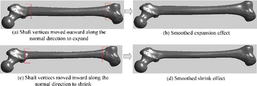
In this step, related regions of the generated model could be further deformed to modify local details, based on known regional parameters. This was a kind of local deformation in which each segmented region deformed independently, just involving the points within a certain region. Each point deformation contained two elements: the scale and the direction of the change. The scaling magnitude hinged on the specific parameter demand, while the moving direction was somewhat difficult to be determined. The work [14] proposed different direction vectors according to different characteristics of different regions. In our proposed method, because the parameter adjustment was small, moving vertices just along the normal direction could cause the corresponding surface to expand outward or shrink inward perfectly.

Although each region was deformed independently, some method such as smoothing function should be adopted to eliminate the discontinuity around the boundary of the deformed region. Each region had a special smoothing function, which generally contained a smoothing range so that the distortion caused by deformation could be eliminated smoothly. For example, for the femoral shaft region, its smoothing function could be defined as$S(p_i)=\{\begin{array}{ll}1\hfill & (x_{p_l}\le x_{p_i}\le x_{p_r})\hfill \\ 0.5+0.5\hspace{0.17em}\cos \left(\frac{\pi }{s_r}(x_{p_i}-x_{p_r})\right)\hfill & x_{p_r}<x_{p_i}\le x_{p_r}\hfill \\ 0.5+0.5\hspace{0.17em}\cos \left(\frac{\pi }{S_l}(x_{p_l}-x_{p_i})\right)\hfill & (x_{p_l}-S_l\le x_{p_i}<x_{p_l})\hfill \end{array}$where $x_{p_i}$ represented the x-coordinate value of point p_i, p_l and p_r were the reference points locating at the left and right boundaries of shaft region, respectively, s_l and s_r were the smoothing range round the left and right boundaries, respectively. The corresponding diagram was shown in Figure 10, and the deformation results were illustrated in Figure 11.

Figure 10. The schematic diagram for the smoothing function of femoral shaft region.

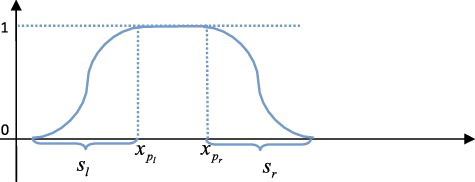
Figure 11. Results of deforming femoral shaft region independently. As shown in (a) and (c), the distortion at both ends of the shaft (see the boxes) was very abrupt, apparent effect was achieved by removing the discontinuity with smoothing function, as illustrated in (b) and (d).

Verifying the validity of the generated model

In order to verify the validity of the generated model, we compared it with the original model from two aspects: (1) the parameter and (2) the shape. The parameter error was easy to obtain. As for the shape error, we used the Hausdorff distance [31], which was a measurement of similarity between two sets of points. Given two finite point sets A = {a₁, a₂,…, a_p} and B = {b₁, b₂,…, b_q}, the Hausdorff distance was defined as$\mathit{H}(\mathit{A},\mathit{B})=\max (\mathit{h}(\mathit{A},\mathit{B}),\mathit{h}(\mathit{A},\mathit{B}))$where$\mathit{h}(\mathit{A},\mathit{B})=\underset{a\in A}{\max }\underset{b\in B}{\min }\Vert a-b\Vert ,\mathit{h}(\mathit{B},\mathit{A})=\underset{b\in B}{\max }\underset{a\in A}{\min }\Vert b-a\Vert$

It had been proved that the Hausdorff distance performs well in the assessment of surface reconstruction [32]. Here, it was used to measure the shape error of the generated model. For the generated model M₁ and the original model M₂, the Hausdorff distance H_i of each segmented region was calculated independently, then the overall Hausdorff distance H_total between the two models was obtained as the weighted sum of each H_i:$H_{\text{total}}(M_1,M_2)={\displaystyle \sum _{i=1}^n{w}_i}\cdot H_i(M_1,M_2)$where n was the total number of segmented regions, H_i was Hausdorff distance between two sets of points which belonged to the ith region of the two models. The weight w_i was set according to specific application. If the region had special requirement for the parameter, the weight was set relatively higher.

Results and discussion

The proposed method was implemented using VC++2010 and Matlab10.0. All femur sample models in STereo Lithography (STL) format were obtained from CT data by 3D reconstruction. They were remeshed to have the same topology as the template model first, and then parameters were calculated based on compatible segmentation. Table 3 lists relevant parameters of all samples in medium group.

Table 3. Relevant parameters of all femur samples in medium group (in mm).

Model	Femur length	Head diameter	Neck length	Neck isthmus diameter	Shaft length	Shaft isthmus diameter	Condyle width
A	434.17	44.86	30.92	31.75	304.11	21.34	70.13
B	436.24	46.04	32.51	31.84	304.57	23.15	70.24
C	440.43	45.98	31.27	35.42	312.32	26.79	75.73
D	455.19	46.87	31.05	36.25	316.63	24.35	76.07
E	460.38	47.69	31.57	36.68	319.56	25.94	77.12
F	461.69	47.78	31.02	37.09	320.94	21.98	77.64
P	450.28	46.77	31.28	35.29	314.91	23.29	75.30
M1	445.99	46.41	31.25	35.33	313.80	24.79	75.48
M2	446.38	47.98	30.97	35.33	313.94	22.78	73.34
T	446.48	48.06	31.22	34.51	312.89	22.69	73.27

In order to test our algorithm of generating a desired femur model according to partial known parameters, one sample model was selected as the test model and some of its morphological parameters were taken as input condition. We then applied our algorithm to generate a new femur model and compared it with the test model. The advantage of doing it this way was that the ground truth data was available to quantify the quality of the generated model. Now let sample T be the test model and select its four measured parameters, respectively, femur length was 446.48 mm, femoral head diameter was 48.06 mm, condyle width was 73.27 mm and shaft isthmus diameter was 22.69 mm. Using these parameters as input condition, the closest femur model could be generated and Figure 12 showed the entire process. The steps involved were given as follows.

Figure 12. Example of generating a desired femur model according to partial known parameters. To generate a model which was the closest to the test model T, first, a rough model M₁ was created through linear interpolation between the group average model P and the best matching model C. Then regions of femoral condyle, head and shaft were further deformed to obtain a refined model M₂.

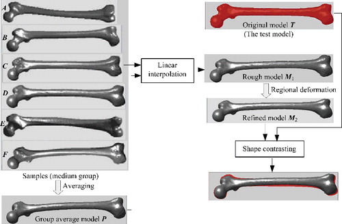
1. The input condition of key parameter (i.e. the femur length) was to be satisfied. First, we chose the prototype for deformation from the medium group according to the key parameter. Then a rough model M₁ with femur length of 445.99 mm was created by linear interpolation at a ratio of 0.57:0.43 between the group average model P and the best matching model C.

2. The input condition of inter-regional parameter (herein was the condyle width) was to be satisfied. Condyle width involves regions of medial condyle and lateral condyle. In order to adjust this parameter more accurately, we deformed the two regions and their border points in different degrees. As a result, the condyle width was adjusted from 75.48 to 73.34 mm, as shown in Figure 13.

   Figure 13. Deformation effect of femoral condyle. The condyle width was adjusted from 75.48 to 73.34 mm.

   

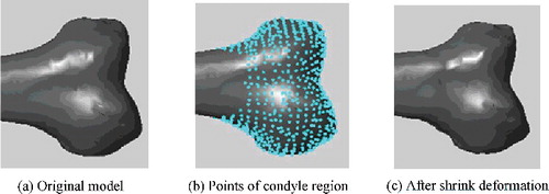
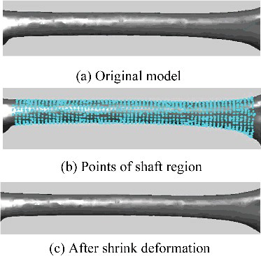
3. The input condition of regional parameter (herein was the femoral head diameter and shaft isthmus diameter) was to be satisfied. By adjusting these two parameters, regions of femoral head and shaft were further deformed separately, as shown in Figures 14 and 15. Eventually, the refined model M₂ was obtained.

   Figure 14. Deformation effect of femoral head. Points of head region moved 0.8 mm along the normal direction, and the head diameter was adjusted from 46.41 to 47.98 mm as a result.

   

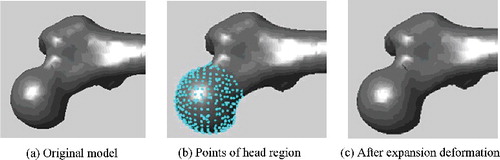
   Figure 15. Deformation effect of femoral shaft. Points of shaft region moved −1.1 mm along the normal direction, and the shaft isthmus diameter was adjusted from 24.79 to 22.78 mm as a result.

   

To evaluate the quality of model M₂, relevant parameters of it were measured. Results showed that parameter differences with the input condition were small, respectively, 0.1 mm for femur length, 0.08 mm for head diameter, 0.07 mm for condyle width and 0.09 mm for shaft isthmus diameter.

To measure the shape error of model M₂, we calculated the Hausdorff distance between T and it. The weight of each region was set as follows: 0.2 for femoral head, lateral condyle, medial condyle and femoral shaft, 0.1 for femoral neck, 0.05 for greater trochanter and lesser trochanter. Table 4 lists the Hausdorff distance for each region and the whole, too. For regions of femoral head, shaft and condyle, whose details were further modified by local deformation, the regional shape error was small. In contrast, the overall shape error was a little bigger, but still within acceptable range to be used in medical practice.

Table 4. Hausdorff distance between the generated model M₂ and the original model T (in mm).

Femoral head	Shaft region	Lateral condyle	Medial condyle	Neck region	Greater trochanter	Lesser trochanter	Whole model
0.0089	0.1813	0.0705	0.0682	0.3011	0.4514	0.5013	0.1435

To further enhance the precision of the generated model, a more comprehensive regional deformation could be performed to achieve more delicate adjustment by increasing the number of input parameters.

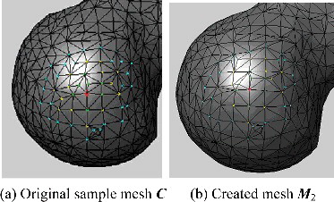
For most deformation applications, it was important to evaluate the mesh quality of the deformed models. In our proposed method, the model was generated by synthetically using overall and regional deformation. On one hand, the overall deformation was implemented through linear interpolation of vertex coordinates between samples, so mesh topology remained unchanged. On the other hand, the magnitude and scope of regional deformation was small and the related vertices moved just along the normal direction, so it would not cause serious mesh distortions. For a certain vertex which belonged to the head region, Figure 16 shows its three-ring neighbourhood on the original sample model C and on the generated model M₂, respectively. It was observed that the mesh quality of the generated model was good, exactly identical to the sample model in topology. However, for some applications especially where numerical models were required, the requirements on mesh quality were higher. In these cases, some smoothing techniques such as Laplacian smoothing method could be used to improve the mesh quality.

Figure 16. A comparison of the three-ring neighbourhood of a given vertex (numbered 228) in the prototype sample and in the created model.

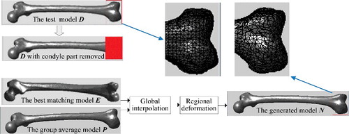
Orthopaedic patients often have some degree of skeleton damage or deformity. In these cases, the generated bone model needs to restore the original anatomy as closely as possible. To achieve this, morphological parameters of undamaged regions of the bone were effectively utilized to generate the anatomically suitable model. Sometimes a few adjustments would be required for the definition of certain parameters, according to the damaged condition of the target bone. Figure 17 shows an example of generating the closest femur model when a part of the bone was damaged. Just as the previous experiment, to obtain the ground truth for result evaluation, we selected sample D as the test model and assumed its condyle part to be damaged. Then morphological parameters on undamaged regions were measured, among which the parameter definition of femur length was adjusted accordingly. Femur length was originally defined as the difference between the maximum and the minimum Z values of all points in the model (assuming the Z-axis along the body height). Since the condyle part was damaged, the definition was adjusted into the difference between the minimum Z value in shaft part and the maximum Z value in the entire model. Next, using the parameters on undamaged regions as input condition, through global interpolation and local deformation, the closest model N was generated in which the condyle part was restored to the normal shape.

Figure 17. Example of generating the anatomically suitable femur model when a part of the bone was damaged. Assuming the condyle part of the test model D was damaged, in order to generate the closest model in which the condyle part could be restored to the normal shape, morphological parameters on undamaged regions were used as input condition, among which the definition of femur length was adjusted accordingly. Then the group average model P and the best matching model E were selected to perform global interpolation, and combining with regional deformation to modify details, the closest model N was generated.

Focusing on the restoration effect of the damaged part, relevant parameters of condyle region in D and N were measured completely. As shown in Table 5, the difference between each parameter was very small. To measure the shape error of the restored region, we calculated the Hausdorff distance of condyle region between D and N. The result was 0.1127, which was clinically acceptable. Due to the inherent structural complexity, there were always some differences in the condyle shape even if the morphological parameters were similar. However, when designing artificial knee joint, it is parameter such as width and anterior–posterior diameter of the condyle that will be of great importance. So a certain degree of shape difference is within acceptable range in medical practice.

Table 5. Relevant parameters of femoral condyle (in mm).

Model	Anterior–posterior diameter of lateral condyle	Anterior–posterior diameter of medial condyle	Width of lateral condyle	Width of medial condyle	Condyle width
D	62.78	59.39	25.29	27.53	76.07
N	62.73	59.03	25.07	27.30	76.21

Our method, however, had some limitations. First, at present only longitudinal parameters were well controlled during the deformation process, some complicated parameters such as shaft curvature radius needs to be more delicately controlled. To solve this problem, the correlation between morphological parameters should be further explored. Second, current sample size was too small, because of limited research time. In future work we plan to collect more bone samples. With increased density of the sample space, we shall be able to greatly improve the accuracy of the generated bone models.

As shown in the experiment results, our proposed method was able to efficiently generate desired femur models merely with partial known parameters as input condition. Even in the cases when a part of the femur bone was damaged, the closest model could be generated in which the damaged part was restored to the normal shape. By testing the parameter error and the shape error, it could be concluded that the generated bone model was anatomically suitable, which was particularly important for orthopaedic surgery and prostheses design. And while we focused on the femur model in this paper, our method had the advantage that it could be extended to other human bone models easily.

Conclusion

In order to quickly generate a 3D model which best suits the patient's femur bone even if a part of the bone was damaged or only partial data about the bone shape was available, this paper synthetically adopted deformation techniques based on morphological parameters. Compared with the existing methods, main advantages of our method were as follows.

1. With a template-related strategy, quick mesh segmentation and parameters calculation for all femur models could be achieved, which provided good foundation for later deformation.

2. Comprehensively applying global and local deformation, our method was flexible and efficient.

3. With the group average model and the best matching sample as reference, the requirements for anatomical characteristics of the generated bone model could be satisfied.

The future work will focus on enhancing the accuracy of the generated bone models. In addition to collecting more samples and further exploring the correlation between morphological parameters, our attention should be paid on other relevant factors such as sex, age, weight and living surroundings of patients which also have influence on the bone shape.

Disclosure statement

No potential conflict of interest was reported by the authors.

Additional information

Funding

This work was supported by the Natural Science Foundation of China [grant number 61472118]; Natural Science Foundation of Jiangsu Province of China [grant number BK20141158]; Science and Technology Program of Jiangsu Province of China [grant number BE2014048]; Fundamental Research Funds for the Central Universities [2013B19214].

References

- He K, Chen Z, Jiang J, et al. Creation of user-defined freeform feature from surface models based on characteristic curves. Comput Ind. 2014;65(4):598–609.
- Majstorovic V, Trajanovic M, Vitkovic N, et al. Reverse engineering of human bones by using method of anatomical features. CIRP Ann-Manuf Technol. 2013;62(1): 167–170.
- He K, Zhao Z, Geng W, et al. Parametric representation and implementation of freeform surface feature based on layered parameters. J Comput-Aided Des Comput Graph. 2014;26(5):826–834.
- Xue W, Dai K, Tang T, et al. Measurement and classification of geometric parameters in Chinese proximal femur. J Biomed Eng. 2002;19(1):84–88.
- Zhang C, Lv H, Zhou D. Chinese normal femur CT measurements and studies about the design of prosthesis. Chinese J Orthop. 1998;18 (8):467–470.
- Zhou Z, Yao Z, Zhen N, et al. Measurement of Chinese proximal femur in X-ray radiography and its implication to the design of artificial total hip. J Shanghai Second Med Univ. 1987;7(1):27–30.
- Lv LW, Meng GW, Gong H, et al. A new method for the measurement and analysis of three-dimensional morphological parameters of proximal male femur. Biomed Res. 2012;23(2):219–226.
- Mahaisavariya B, Sitthiseripratip K, Tongdee T, et al. Morphological study of the proximal femur: a new method of geometrical assessment using 3-dimensional reverse engineering. Med Eng Phys. 2002;24(9):617–622.
- Dong X, Zheng GY. Fully automatic determination of morphological parameters of proximal femur from calibrated fluoroscopic images through particle filtering. In: Póvoa De Varzim, editor. Proceedings of the third International Conference on Image Analysis and Recognition. Berlin: Springer-Verlag; 2006. p. 535–546.
- Blanz V, Vetter T. A morphable model for the synthesis of 3D faces[C]. Proceedings of the 26th annual conference on Computer graphics and interactive techniques. New York (NY): ACM Press/Addison-Wesley Publishing Co.; 1999. p. 187–194.
- Allen B, Curless B, Popović Z. The space of human body shapes: reconstruction and parameterization from range scans. ACM Trans Graph. 2003;22(3):587–594.
- Yoo DJ. Three-dimensional morphing of similar shapes using a template mesh. Int J Precis Eng Manuf. 2009;10(1):55–66.
- Liao S. 3D reconstruction of medical model and generation of volume mesh based on deformation [dissertation]. Zhejiang: Zhejiang University; 2008.
- Park BK, Bae JH, Koo BY, et al. Function-based morphing methodology for parameterizing patient-specific models of human proximal femurs. Comput-Aided Des. 2014;51(7):31–38.
- Sigal IA, Yang H, Roberts MD, et al. Morphing methods to parameterize specimen-specific finite element model geometries. Biomechanics. 2010;43(2):254–262.
- Katz S, Leifman G, Tal A. Mesh segmentation using feature point and core extraction. Visual Comput. 2005;21(8–10):649–658.
- Agathos A, Pratikakis I, Perantonis S, et al. Protrusion-oriented 3D mesh segmentation. Visual Comput. 2010;26(1):63–81.
- Lin J, Lu T, Yang Y, et al. Mesh Segmentation by Local Depth (PDF)[M]. 2010.
- Zhang C, Zhang N, Li C, et al. Marker-Controlled Perception-Based Mesh Segmentation[M]// Marker-controlled perception-based mesh segmentation. 2005;390–393.
- Koschan AF. Perception-based 3D triangle mesh segmentation using fast marching watersheds[J]. 2003;2:27–32.
- Zhang L, Liu L, Ji Z, et al. Manifold Parameterization. Advances in Computer Graphics 2006;4035:160–171.
- Sorkine O, Cohen-Or D, Lipman Y, et al. Laplacian surface editing [C]. In: Scopigno R, Zorin D, editors. Proceedings of Eurographics/ACM SIGGRAPH Symposium on Geometry Processing, New York (NY): ACM Press; 2004. p. 175–184.
- Besl PJ, Mckay ND. A method for registration of 3-D shapes. IEEE Trans Pattern Anal Mach Intell. 1992;14(2):239–25.
- Arnone J. A comprehensive simulation-based methodology for the design and optimization of orthopaedic internal fixation implants [dissertation]. Missouri: The University of Missouri; 2011.
- Hao T, Yu B, Hao Z, et al. Three-dimensional digital measurement of fixed parameters of the less invasive stable system fixation. JClin Rehab Tissue Eng Res. 2012;16(13):2292–2295.
- Wang H, Long T, Cui H, et al. Morphological measurements of the proximal tibia and knee replacement. J Clin Rehab Tissue Eng Res. 2011;52(15):9847–9850.
- Zou L, Zhan C, Shi B, et al. Measurement and clinical significance of geometric parameters of the knee joint in normal Chinese people. Anat Clin. 2010;15(4):243–245.
- Park JM, Im GI. The correlations of the radiological parameters of hip dysplasia and proximal femoral deformity in clinically normal hips of a Korean population. Clin Orthop Surg. 2011;3:121–127.
- Fatih Y, Nurcan I, Bilal B, et al. Is there any relation between distal parameters of the femur and its height and width?. Surg Radiol Anat. 2012;34(2):125–132.
- Chen X, He K, Chen Z, et al. Quick construction of femoral model using surface feature parameterization. Mol Cell Biomech. 2015;12(2):123–146.
- Daniel PH, Gregory AK, Willian JR. Comparing images using the Hausdorff distance. IEEE Trans Pattern Anal and Mach Intell. 1993;15(9):850–863.
- He KJ, Wang L, Chen ZM, et al. Reconstruction and featurization of local region based on CAD surface models. Comput Integr Manuf Syst. 2014;20(10):2360–2368.