Quantile normalization for combining gene-expression datasets

ABSTRACT

Our research aimed to improve survival prediction by combining gene expression datasets, and to apply molecular signatures across different datasets. Many methods have previously been developed to remove unwanted variations among datasets and maintain the wanted factor variations. However, for inter-study validation (ISV) research, a whole dataset is set aside for testing, and the statuses of wanted factors are assumed unknown for the whole dataset; thus, regression cannot be used to determine the unwanted variations for this dataset. In this study, quantile normalization (QN) was utilized to remove the unwanted dataset variations, after which the adjusted datasets were used for classification. It was observed that the datasets formed by QN combination in the study of ISV had superior prediction performance compared to the datasets combined by other methods. Combining datasets using QN could improve the prediction performance for the study of ISV.

KEYWORDS:

• Quantile normalization
• gene expression
• dataset
• combination
• prediction
• inter-study validation

Introduction

Microarray gene expression technology provides a systematic approach to cancer classification [1,2]. Many studies have aimed to improve survival prediction by combining gene expression datasets, and to apply molecular signatures across different datasets [3–8]. However, inter-dataset variation hindered these attempts [9–11].

Some methods have been developed to remove unwanted dataset variations (or batch variations) and maintain the wanted factor variations [12–15]. For example, in the removal of unwanted variation (RUV) model, the gene expression values are assumed as Y = Xβ + Wα + ϵ, where X represents the factors of interest (e.g. the predictive factors), W, the unwanted factors (e.g. the dataset factors or batch factors), and ϵ, an arbitrary amount of noise (see details in section Materials and methods) [15].

The RUV model is effective for the study of intra-dataset validation, in which some samples or one sample of the datasets is set aside for testing, and the remaining part (each dataset has samples in this part) is utilized for training. In the training process (both wanted and unwanted factors, X and W, are assumed known for the training samples), the unwanted variations, α, can be determined for every dataset by regression, and then be removed.

However, for the study of inter-study validation (ISV), a whole dataset is set aside for testing, and the record of X is assumed unknown for the whole dataset; thus, the unwanted variations cannot be determined for this dataset in the regression.

In this regard, quantile normalization (QN), a global adjustment method that assumes the statistical distribution of each sample is the same [16], is used, as it does not require the record of X. The assumption is justified in many biomedical applications in which only a minority of genes are expected to be differentially expressed (not including differential mythylation). QN has been shown to be effective for normalizing GeneChip arrays, and was integrated into RMA (robust multi-array analysis), the software for raw data processing [17].

In this study, QN was utilized to remove unwanted dataset variations. It was utilized to combine simulated or real datasets, after which the datasets were used for classification. The classification performance was evaluated and compared with those of other methods.

Materials and methods

Simulated datasets

A Monte Carlo setup similar to reference [18] was used. In each simulation, five datasets that contain 40, 60, 80, 100 and 120 samples of class 0, and 200, 180, 160, 140 and 120 samples of class 1 were generated using multivariate normal distributions with class-specific mean vectors and common covariance matrices. The simulations were performed with n = 1000 genes (variables), and the first n₁ = 50 were differentially expressed between classes with a mean difference of 1. The remaining 950 genes had the same mean for each class. For the common covariance matrix, Structures 1–3 as defined in reference [18] were used:$\text{Structure}1:\left[\begin{array}{ll}{\Sigma }_{11}& 0\\ 0^{\prime }& I_{n-n_1}\end{array}\right],$$\text{Structure}2:\left[\begin{array}{ll}{\Sigma }_{11}& 0\\ 0^{\prime }& {\Sigma }_{22}\end{array}\right],$$\text{Structure}3:\left[\begin{array}{ll}{\Sigma }_{11}& {\Sigma }_{12}\\ {{\Sigma }^{\prime }}_{12}& {\Sigma }_{22}\end{array}\right],$where ${\Sigma }_{11}$ and ${\Sigma }_{22}$ are $n_1\times n_1$ and $(n-n_1)\times (n-n_1)$ intra-class correlation matrices for $n_1$ informative genes and for $n-n_1$ noninformative genes, respectively. ${\Sigma }_{12}$ is the $n_1\times (n-n_1)$ correlation matrix between informative and noninformative genes and $I_{n-n_1}$ is the $(n-n_1)\times (n-n_1)$ identity matrix. The gene–gene correlations were set as 0.5. One hundred simulation replicates were performed for each structure.

Real datasets

Gene-expression datasets of breast cancer with a record of endocrine responsiveness (ER) status were pre-selected from the Gene Expression Omnibus (http://www.ncbi.nlm.nih.gov/geo [19]). The following criteria were also applied: (1) datasets were in the same platform (GPL96, which contains 22215 probe-sets); (2) probe intensities were quantified with the same method (MAS 5.0); and (3) sample numbers were greater than 100; (4) datasets have both ER+ and ER− samples. In addition, datasets with overlapped samples were excluded. Finally, six datasets [20–25] were included (see Table 1), consisting of 1640 samples (1103 ER+ and 537 ER−).

Table 1. Gene expression datasets.

Source	Dataset	N (ER +/−)
Wang et al. [20]	GSE2034	286 (209/77)
Ivshina et al. [21]	GSE4922	245 (211/34)
Desmedt et al. [22]	GSE7390	198 (134/64)
Shi et al. [23]	GSE20194	278 (164/114)
Hatzis et al. [24]	GSE25066	496 (296/200)
Nagalla et al. [25]	GSE45255	137 (89/48)

N: number of samples.

QN combination

QN was chosen in this study to remove unwanted dataset variations before combining the datasets. Normalization was achieved by forcing the observed distributions to be the same and the average distribution, obtained by taking the average of each quantile across samples, was used as the reference [16]. It has been successfully used to remove batch effects for microarray datasets. In this study, it was used to remove inter-dataset variations. It was conducted in MATLAB according to an algorithm previously described [16].

RUV combination

RUV combination was also chosen for comparison. In the RUV model, the gene expression values are assumed as Y = Xβ + Wα + ϵ, with Y ∈ R^m×n, X ∈ R^m×p, β ∈ R^p×n, W ∈ R^m×k, α ∈ R^k×n, and ϵ ∈ R^m×n, where Y is the observed matrix of expression of n genes for m samples, X represents the p factors of interest, W, the k unwanted factors, and ϵ, an arbitrary amount of noise [15].

According to the RUV model, if both the factor matrices X and W are known, the wanted variations (β) and unwanted variations (α) can be determined by regression. The adjusted gene expression values can be obtained by removing the unwanted variations, Y* = Y − Wα.

In the RUV model, the element (W)_ij is set to 1 if the i-th sample belongs to the j-th dataset, or set to 0 otherwise; the element (X)_ij is set to 1 or −1 if the i-th sample belongs to one of two statuses of the j-th factor. For the study of ISV, a whole dataset is set aside for testing, and the record of X is assumed unknown for the whole dataset; thus, the unwanted variation, α, as well as the adjusted value, Y*, cannot be determined for this dataset in the regression. The ISV may not be performed. Alternatively, the element (X)_ij may be set to a median value, 0, if the status of the j-th factor was unknown for the i-th sample.

RUV combination was conducted in MATLAB according to the above descriptions.

Classifiers

There are correlations between genes [26]. Therefore, correlation-based classifiers were chosen, and utilized to predict the status of wanted factors.

SVM (support vector machine) classification is a correlation-based binary classification that uses selected variables (features) and fits an optimal hyperplane between two classes by maximizing the margin between the closest points [27,28]. This classification was implemented in MATLAB using the functions svmtrain and svmclassify.

The ensemble of random subspace (RS) Fisher linear discriminant (FLD) classifier (referred to as enRS-FLD) is another correlation-based classifier, the decision of which is taken by averaging the decisions of the base classifiers (FLD classifiers) working in the lower dimensional subspaces [29]. The enRS-FLD classifier was also chosen, and was conducted in MATLAB according to the algorithm described in reference [29]. The parameters employed by these authors were also used. The dimension of the subspaces, k, was set to (N − 2)/2 to optimize the classification, where N was the number of samples in the training dataset. The number of subspaces, M, was set to 100 (for simulated datasets) or 1000 (for real datasets).

Classification performance

The F1-measure and accuracy [30,31] were used to evaluate the classification performance.

For the study of intra-dataset validation, 5-fold cross-validation (CV) was used. For the study of inter-dataset validation, leave-dataset-out cross-validation (LDOCV) was used.

In the process of validation, one fold or one dataset was set aside in turn for testing, and the wanted factors were assumed unknown for them; the remaining part was utilized for training. Then both the testing and training set were combined and adjusted by QN combination or RUV combination, and the adjusted training set was used to train the classifier and predict the wanted factors for the testing set.

Results and discussion

Intra-dataset validation for simulated datasets

For each of the three structures, 100 replicates were generated. In each replicate, five datasets were generated. Intra-dataset validation (5-fold CV, 100 random splits) was carried out using each dataset individually or using the five datasets combined by RUV or QN combination. After the validation, further testing was carried out using 100 times larger datasets. The F1-measure and accuracy were computed for each dataset and averaged over the 100 splits and the 100 replicates. The results are shown in Figure 1 and Table 2 (see also Figure S1, Tables S1 and S2 in the Online Supplemental Data). It was observed that the classification performance for Structure 3 was superior to those for the other two structures. The classifiers benefited from the correlations between the informative and non-informative genes [32]. It was observed that the performance of RUV combination was superior to that of the non-combination approach for datasets of Structure 3; and inferior for datasets of Structures 1 and 2. This might be due to the shift of the mean in the RUV combination. The performance of QN combination was inferior to RUV combination for datasets of Structure 2, and near to RUV combination for datasets of the other two structures.

Figure 1. Classification performance in intra-dataset validation (5-fold CV, 100 splits) for simulated datasets.

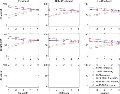
Table 2. Classification performance in intra-dataset validation (5-fold CV) for simulated datasets.

		Individual datasets			RUV-combined datasets			QN-combined datasets
Classifier	Dataset	F1-measure1	F1-measure0	Accuracy	F1-measure1	F1-measure0	Accuracy	F1-measure1	F1-measure0	Accuracy
SVM	Structure 1^a	80.65 ± 1.06^b	54.10 ± 2.64	75.26 ± 1.29	75.79 ± 1.16(−)^c	51.61 ± 1.99	68.46 ± 1.45(−)	76.37 ± 1.12	52.47 ± 2.01	69.32 ± 1.43
	Test^d	80.76 ± 0.33	54.12 ± 1.13	75.38 ± 0.37	76.23 ± 0.62(−)	52.26 ± 1.07	69.50 ± 0.72(−)	76.39 ± 0.62	52.41 ± 1.06	69.32 ± 0.71
	Structure 2	81.01 ± 1.14	55.69 ± 2.42	75.72 ± 1.34	75.97 ± 1.30(−)	51.97 ± 2.21	68.69 ± 1.64(−)	71.39 ± 1.20(−)^e	43.80 ± 1.97(−)	62.91 ± 1.51(−)
	Test	81.15 ± 0.37	55.98 ± 1.17	75.91 ± 0.37	76.42 ± 0.65(−)	52.69 ± 1.07(−)	69.73 ± 0.74(−)	71.43 ± 0.61(−)	43.76 ± 0.89(−)	62.94 ± 0.66(−)
	Structure 3	99.98 ± 0.03	99.91 ± 0.13	99.97 ± 0.04	100.00	100.00	100.00	100.00	100.00	100.00
	Test	99.979 ± 0.007	99.916 ± 0.036	99.968 ± 0.012	99.998 ± 0.001(+)	99.997 ± 0.002(+)	99.998 ± 0.001(+)	99.998 ± 0.001	99.996 ± 0.003	99.998 ± 0.002
enRS-FLD	Structure 1	81.68 ± 0.95	60.87 ± 2.28	76.92 ± 1.14	76.20 ± 1.19(−)	55.76 ± 1.90(−)	69.79 ± 1.44(−)	77.31 ± 1.07	56.94 ± 1.90	71.17 ± 1.35
	Test	81.77 ± 0.23	60.90 ± 0.70	77.02 ± 0.21	76.67 ± 0.47(−)	56.34 ± 0.69(−)	70.83 ± 0.49(−)	77.34 ± 0.42	56.88 ± 0.68	71.18 ± 0.45
	Structure 2	81.54 ± 1.00	60.52 ± 2.08	76.71 ± 1.17	76.19 ± 1.23(−)	55.65 ± 1.92(−)	69.74 ± 1.48(−)	72.90 ± 1.28	48.93 ± 2.03(−)	65.45 ± 1.58
	Test	81.67 ± 0.29	60.72 ± 0.75	76.87 ± 0.26	76.67 ± 0.49(−)	56.39 ± 0.66(−)	70.83 ± 0.52(−)	72.96 ± 0.53(−)	48.88 ± 0.73(−)	65.49 ± 0.55(−)
	Structure 3	99.99 ± 0.02	99.94 ± 0.08	99.98 ± 0.03	100.00	99.98 ± 0.04	99.99 ± 0.02	100.00	100.00	100.00
	Test	99.985 ± 0.004	99.941 ± 0.019	99.977 ± 0.006	99.997 ± 0.001(+)	99.993 ± 0.002(+)	99.996 ± 0.001(+)	99.998 ± 0.001	99.996 ± 0.002	99.997 ± 0.001

Subscript 1: class 1. Subscript 0: class 0.

^a 100 simulation replicates were generated for each structure. In each replicate, five datasets were generated and randomly split (100 times) for cross-validation (see text).

^b Each value (in percent) is averaged over the 100 replicates, the five datasets, and the 100 splits. A standard error (the number after ±) is estimated from the 100 replicates.

^c The symbol in the brackets indicates if the performance of RUV combination is statistically significantly superior (+) or inferior (−) to that of non-combination with 95% confidence level.

^d For the five datasets, 100 times larger datasets were generated for further testing.

^e The symbol in the brackets indicates if the performance of QN combination is statistically significantly superior (+) or inferior (−) to that of RUV combination with 95% confidence level.

Inter-dataset validation for simulated datasets

Inter-dataset validation (LDOCV) was carried out using datasets combined by RUV combination and QN combination. The F1-measure and accuracy were computed for each dataset and averaged over the 100 replicates. The results are shown in Figure 2 and Table 3 (see also Figure S2, Tables S3 and S4 in the Online Supplemental Data). The inter-dataset validation was found to exhibit declined performance compared to the intra-dataset validation when the datasets were combined by RUV combination, especially when a dataset was unbalanced. However, the inter-dataset validation using datasets combined by QN combination outperformed the use of datasets combined by RUV combination, especially for datasets of Structures 1 and 3, owing to the improvement of the classification performance for the unbalanced datasets; and had performance similar to the intra-dataset validation using datasets combined by QN combination.

Figure 2. Classification performance in inter-dataset validation (LDOCV) for simulated datasets.

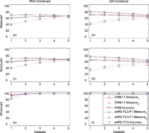
Table 3. Classification performance in inter-dataset validation (LDOCV) for simulated datasets.

		RUV-combined datasets			QN-combined datasets
Classifier	Dataset	F1-measure1	F1-measure0	Accuracy	F1-measure1	F1-measure0	Accuracy
SVM	Structure 1	70.82 ± 1.44^a	53.65 ± 2.06	64.67 ± 1.67	75.94 ± 1.32(+)^b	51.46 ± 2.46	68.49 ± 1.71(+)
	Test	70.82 ± 0.86	53.74 ± 0.91	64.73 ± 0.84	76.05 ± 0.60(+)	51.79 ± 1.05(−)	68.66 ± 0.72(+)
	Structure 2	71.01 ± 1.51	54.10 ± 2.25	64.93 ± 1.77	70.94 ± 1.51	43.16 ± 2.34(−)	62.16 ± 1.81
	Test	70.99 ± 0.90	54.06 ± 0.90	64.93 ± 0.87	71.05 ± 0.63	43.21 ± 0.79(−)	62.23 ± 0.66(−)
	Structure 3	99.22 ± 0.19	96.91 ± 0.63	98.75 ± 0.29	100.00(+)	99.99 ± 0.03(+)	100.00(+)
	Test	99.21 ± 0.10	96.90 ± 0.34	98.75 ± 0.15	100.00(+)	100.00(+)	100.00(+)
enRS-FLD	Structure 1	70.18 ± 1.42	56.68 ± 1.79	65.22 ± 1.55	77.22 ± 1.39(+)	56.54 ± 2.37	70.86 ± 1.73(+)
	Test	70.08 ± 0.78	56.58 ± 0.53	65.14 ± 0.68	77.21 ± 0.45(+)	56.61 ± 0.65	70.87 ± 0.48(+)
	Structure 2	70.12 ± 1.46	56.51 ± 1.74	65.12 ± 1.56	72.60 ± 1.49	48.51 ± 2.30(−)	64.96 ± 1.77
	Test	70.12 ± 0.78	56.60 ± 0.51	65.17 ± 0.69	72.76 ± 0.55(+)	48.56 ± 0.72(−)	65.09 ± 0.57
	Structure 3	98.86 ± 0.22	95.83 ± 0.65	98.22 ± 0.33	100.00(+)	100.00(+)	100.00(+)
	Test	98.84 ± 0.12	95.76 ± 0.37	98.19 ± 0.18	100.00(+)	100.00(+)	100.00(+)

^a The standard error is estimated from the 100 simulation replicates.

^b The symbol in the brackets indicates if the performance of QN combination is statistically significantly superior or inferior to that of RUV combination.

Intra-dataset validation for real datasets

For real datasets, intra-dataset validation (5-fold CV) was carried out using each dataset individually or the six datasets combined by RUV or QN combination. The F1-measure and accuracy were computed for each dataset. The results are shown in Figure 3 and Table 4. Overall, it was observed that the RUV combined datasets performed more effectively than the individual datasets, and the QN combined datasets performed somewhat better than the RUV combined datasets.

Figure 3. Classification performance in intra-dataset validation (5-fold CV, 100 splits) for real datasets.

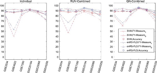
Table 4. Classification performance in intra-dataset validation (5-fold CV) for real datasets.

		Individual datasets			RUV-combined datasets			QN-combined datasets
Classifier	Dataset	F1-measure1	F1-measure0	Accuracy	F1-measure1	F1-measure0	Accuracy	F1-measure1	F1-measure0	Accuracy
SVM	GSE2034	91.79 ± 0.64^a	77.27 ± 1.79	87.94 ± 0.93	92.40 ± 0.50	80.91 ± 1.22	89.13 ± 0.70	91.62 ± 0.59	78.12 ± 1.58	87.88 ± 0.86
	GSE4922	92.34 ± 0.52	39.28 ± 5.00	86.40 ± 0.93	92.66 ± 0.53	46.69 ± 4.49	87.10 ± 0.93	93.56 ± 0.57	60.76 ± 4.52(+)	88.94 ± 1.00
	GSE7390	91.50 ± 0.62	81.55 ± 1.44	88.35 ± 0.86	90.82 ± 0.71	81.02 ± 1.51	87.63 ± 0.96	90.95 ± 0.69	81.48 ± 1.50	87.84 ± 0.93
	GSE20194	93.14 ± 0.71	90.00 ± 1.11	91.86 ± 0.86	91.77 ± 1.08	88.16 ± 1.59	90.29 ± 1.28	95.44 ± 0.68(+)	93.44 ± 0.99(+)	94.62 ± 0.81(+)
	GSE25066	89.64 ± 0.46	84.71 ± 0.71	87.65 ± 0.56	87.91 ± 1.04	81.71 ± 1.58	85.45 ± 1.24	92.69 ± 0.55(+)	89.51 ± 0.79(+)	91.39 ± 0.64(+)
	GSE45255	87.37 ± 1.16	72.30 ± 2.45	82.66 ± 1.55	87.83 ± 0.85	71.96 ± 2.21	83.03 ± 1.21	86.84 ± 1.17	71.46 ± 2.86	81.99 ± 1.62
	Average	90.96 ± 0.31	74.18 ± 1.05	87.48 ± 0.42	90.57 ± 0.32	75.07 ± 0.89	87.10 ± 0.40	91.85 ± 0.31(+)	79.13 ± 0.98(+)	88.78 ± 0.42(+)
enRS-FLD	GSE2034	91.78 ± 0.48	78.39 ± 1.37	88.09 ± 0.71	93.33 ± 0.29(+)	83.03 ± 0.80(+)	90.42 ± 0.42(+)	92.83 ± 0.24	81.26 ± 0.79	89.63 ± 0.37
	GSE4922	92.65 ± 0.46	52.71 ± 3.34	87.28 ± 0.80	94.15 ± 0.37(+)	66.39 ± 2.63(+)	90.03 ± 0.64(+)	93.99 ± 0.33	65.61 ± 2.36	89.77 ± 0.58
	GSE7390	92.36 ± 0.66	84.19 ± 1.36	89.70 ± 0.88	91.47 ± 0.48	82.34 ± 0.97	88.50 ± 0.64	91.59 ± 0.38	82.61 ± 0.78	88.67 ± 0.50
	GSE20194	92.79 ± 0.70	89.52 ± 1.05	91.46 ± 0.84	95.90 ± 0.73(+)	93.87 ± 1.12(+)	95.08 ± 0.88(+)	96.69 ± 0.63	95.23 ± 0.93	96.09 ± 0.75
	GSE25066	90.40 ± 0.36	86.04 ± 0.58	88.62 ± 0.45	92.82 ± 0.32(+)	89.60 ± 0.48(+)	91.50 ± 0.38(+)	93.08 ± 0.31	90.14 ± 0.46	91.86 ± 0.36
	GSE45255	87.04 ± 1.14	73.31 ± 2.27	82.56 ± 1.48	90.41 ± 0.73(+)	79.29 ± 1.70(+)	86.89 ± 1.01(+)	89.87 ± 0.82	77.62 ± 2.00	86.06 ± 1.16
	Average	91.17 ± 0.29	77.36 ± 0.77	87.95 ± 0.38	93.01 ± 0.23(+)	82.42 ± 0.63(+)	90.41 ± 0.31(+)	93.01 ± 0.23	82.08 ± 0.61	90.35 ± 0.31

Subscript 1: ER+; Subscript 0: ER−.

^a The standard error is estimated from the 100 CV splits.

Inter-dataset validation for real datasets

Inter-dataset validation (LDOCV) was carried out using datasets combined by RUV combination and QN combination. The F1-measure and accuracy were computed for each dataset. The results are shown in Figure 4 and Table 5. It was also observed that the inter-dataset validation had a declined performance compared to the intra-dataset validation when the datasets were combined by RUV combination. The performance of inter-dataset validation using datasets combined by QN combination was superior to that using datasets combined by RUV combination, owing to the improvement of classification performance for the unbalanced datasets. Even if datasets having only ER+ (or ER−) or having only one sample were included, QN combination would work well, while the RUV combination would not work.

Figure 4. Classification performance in inter-dataset validation (LDOCV) for real datasets.

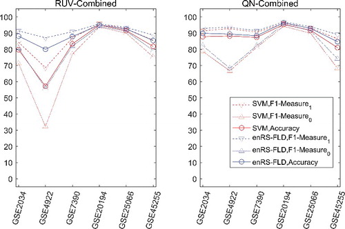
Table 5. Classification performance in inter-dataset validation (LDOCV) for real datasets.

		RUV-combined datasets			QN-combined datasets
Classifier	Dataset	F1-measure1	F1-measure0	Accuracy	F1-measure1	F1-measure0	Accuracy
SVM	GSE2034	84.32 ± 2.06^a	71.29 ± 2.83	79.72 ± 2.41	91.40 ± 1.23(+)	78.79 ± 2.82	87.76 ± 1.69(+)
	GSE4922	68.67 ± 2.78	32.26 ± 2.89	57.14 ± 2.94	92.80 ± 1.31(+)	66.67 ± 4.64(+)	88.16 ± 2.04(+)
	GSE7390	86.96 ± 2.52	76.92 ± 3.87	83.33 ± 3.01	90.49 ± 1.95	81.20 ± 3.53	87.37 ± 2.49
	GSE20194	95.76 ± 0.99	93.81 ± 1.45	94.96 ± 1.17	96.07 ± 0.94	94.22 ± 1.43	95.32 ± 1.13
	GSE25066	92.68 ± 1.01	89.95 ± 1.31	91.53 ± 1.14	93.02 ± 1.04	89.88 ± 1.45	91.73 ± 1.21
	GSE45255	85.55 ± 3.15	75.25 ± 5.16	81.75 ± 3.82	86.46 ± 2.25	68.29 ± 5.98	81.02 ± 3.21
	Average	85.66 ± 0.90	73.25 ± 1.37	81.40 ± 1.07	91.71 ± 0.70(+)	79.84 ± 1.62(+)	88.56 ± 0.95(+)
enRS-FLD	GSE2034	91.41 ± 1.44	80.68 ± 2.81	88.11 ± 1.90	92.91 ± 1.33	82.21 ± 2.96	89.86 ± 1.83
	GSE4922	87.07 ± 1.78	55.86 ± 3.67	80.00 ± 2.47	93.63 ± 1.30(+)	68.29 ± 5.45	89.39 ± 2.09(+)
	GSE7390	90.84 ± 1.68	82.09 ± 3.59	87.88 ± 2.27	91.39 ± 1.52	82.17 ± 3.00	88.38 ± 2.00
	GSE20194	95.68 ± 1.26	93.97 ± 2.58	94.96 ± 1.70	96.95 ± 0.97	95.61 ± 1.38	96.40 ± 1.14
	GSE25066	93.50 ± 1.16	91.25 ± 1.83	92.54 ± 1.41	93.98 ± 0.92	91.48 ± 1.25	92.94 ± 1.05
	GSE45255	88.76 ± 2.44	79.17 ± 4.74	85.40 ± 3.17	89.12 ± 1.93	74.07 ± 5.58	84.67 ± 2.86
	Average	91.21 ± 0.73	80.50 ± 1.44	88.15 ± 0.96	93.00 ± 0.56	82.31 ± 1.57	90.28 ± 0.80

^a The standard error is estimated assuming that the numbers of true positive and true negative samples are binomially distributed.

The performance of inter-dataset validation using datasets combined by QN combination was superior to that of intra-dataset validation using individual datasets, therefore higher level of statistical significance was achieved by QN combination. Inter-dataset validation using datasets combined by QN combination had performance similar to or somewhat better than that of intra-dataset validation using datasets combined by RUV combination. This challenged the conventional view that the performance of inter-dataset validation was poorer than that of intra-dataset validation [11,33]. In future research, it may be need to take into account the unbalanced datasets and QN normalization.

Conclusions

In intra-dataset validation, combining datasets using the RUV model had positive impact compared to the individual datasets for simulated datasets of Structure 3 and real datasets. In inter-dataset validation, combining datasets using QN had positive impact compared to combining datasets using the RUV model. Combining datasets using QN could improve the prediction performance for the study of ISV. The prediction performance of inter-dataset validation using datasets combined by QN was higher than that of intra-dataset validation using individual datasets, for simulated datasets of Structure 3 and real datasets. The inter-dataset variations were removed by QN and higher performance was obtained.

Acknowledgments

The authors are grateful to the authors of the datasets and those responsible for the availability of the data.

Disclosure statement

The authors declare no conflict of interest.

References

- Golub TR, Slonim DK, Tamayo P, et al. Molecular classification of cancer: class discovery and class prediction by gene expression monitoring. Science. 1999;286:531–537.
- Ross DT, Scherf U, Eisen MB, et al. Systematic variation in gene expression patterns in human cancer cell lines. Nat Genet. 2000;24:227–234.
- Autio R, Kilpinen S, Saarela M, et al. Comparison of Affymetrix data normalization methods using 6,926 experiments across five array generations. BMC Bioinformatics. 2009;10(Suppl. 1):S24.
- Xu L, Tan AC, Winslow RL, et al. Merging microarray data from separate breast cancer studies provides a robust prognostic test. BMC Bioinformatics. 2008;9:125.
- van Vliet MH, Reyal F, Horlings HM, et al. Pooling breast cancer datasets has a synergetic effect on classification performance and improves signature stability. BMC Genomics. 2008;9:375.
- Xu L, Tan AC, Naiman DQ, et al. Robust prostate cancer marker genes emerge from direct integration of inter-study microarray data. Bioinformatics. 2005;21:3905–3911.
- Kim K-Y, Ki D, Jeung H-C, et al. Improving the prediction accuracy in classification using the combined data sets by ranks of gene expressions. BMC Bioinformatics. 2008;9:283.
- Kim S-Y. Effects of sample size on robustness and prediction accuracy of a prognostic gene signature. BMC Bioinformatics. 2009;10:147.
- Yasrebi H, Sperisen P, Praz V, et al. Can survival prediction be improved by merging gene expression data sets? PLoS ONE. 2009;4(10):e7431.
- Bevilacqua V, Pannarale P, Abbrescia M, et al. Comparison of data-merging methods with SVM attribute selection and classification in breast cancer gene expression. BMC Bioinformatics. 2012;13(Suppl. 7):S9.
- Ma S, Sung J, Magis AT, et al. Measuring the effect of inter-study variability on estimating prediction error. PLoS ONE. 2014;9(10):e110840.
- Johnson WE, Li C, Rabinovic A. Adjusting batch effects in microarray expression data using empirical Bayes methods. Biostatistics. 2007;8(1):118–127.
- Leek JT, Storey JD. Capturing heterogeneity in gene expression studies by surrogate variable analysis. PLoS Genet. 2007;3:e161.
- Gagnon-Bartsch JA, Speed TP. Using control genes to correct for unwanted variation in microarray data. Biostatistics. 2012;13:539–552.
- Jacob L, Gagnon-Bartsch JA, Speed TP. Correcting gene expression data when neither the unwanted variation nor the factor of interest are observed. Biostatistics. 2016;17(1):16–28.
- Hicks SC, Irizarry RA. Quantro: a data-driven approach to guide the choice of an appropriate normalization method. Genome Biol. 2015;16(1):117.
- Irizarry RA, Hobbs B, Collin F, et al. Exploration, normalization, and summaries of high density oligonucleotide array probe level data. Biostatistics. 2003;4:249–264.
- Kim KI, Simon R. Probabilistic classifiers with high-dimensional data. Biostatistics. 2011;12(3):399–412.
- Gene Expression Omnibus. Available from: http://www.ncbi.nlm.nih.gov/geo/browse/
- Wang Y, Klijn JG, Zhang Y, et al. Gene-expression profiles to predict distant metastasis of lymph-node-negative primary breast cancer. Lancet. 2005;365(9460):671–679.
- Ivshina AV, George J, Senko O, et al. Genetic reclassification of histologic grade delineates new clinical subtypes of breast cancer. Cancer Res. 2006;66(21):10292–10301.
- Desmedt C, Piette F, Loi S, et al. Strong time dependence of the 76-gene prognostic signature for node-negative breast cancer patients in the transbig multicenter independent validation series. Clin Cancer Res. 2007;13:3207–3214.
- Shi L, Campbell G, Jones WD, et al. The MicroArray Quality Control (MAQC)-II study of common practices for the development and validation of microarray-based predictive models. Nat Biotechnol. 2010;28(8):827–838.
- Hatzis C, Pusztai L, Valero V, et al. A genomic predictor of response and survival following taxane-anthracycline chemotherapy for invasive breast cancer. J Am Med Assoc. 2011;305:1873–1881.
- Nagalla S, Chou JW, Willingham MC, et al. Interactions between immunity, proliferation and molecular subtype in breast cancer prognosis. Genome Biol. 2013;14:R34.
- Jong VL, Novianti PW, Roes KC, et al. Exploring homogeneity of correlation structures of gene expression datasets within and between etiological disease categories. Stat Appl Genet Mol Biol. 2014;13(6):717–732.
- Novianti PW, Jong VL, Roes KC, et al. Factors affecting the accuracy of a class prediction model in gene expression data. BMC Bioinformatics. 2015;16:199.
- Statnikov A, Aliferis CF, Tsamardinos I, et al. A comprehensive evaluation of multicategory classification methods for microarray gene expression cancer diagnosis. Bioinformatics. 2005;21(5):631–643.
- Durrant R, Kabán A. Random projections as regularizers: learning a linear discriminant from fewer observations than dimensions. Mach Learn. 2015;99:257–286.
- Xie S, Li P, Jiang Y, et al. A discriminative method for protein remote homology detection based on N-Gram. Genet Mol Res. 2015;14(1):69–78.
- Tripathy A, Agrawal A, Kumar Rath SK. Classification of sentiment reviews using n-gram machine learning approach. Expert Syst Appl. 2016;57:117–126.
- Pan M, Zhang J. Correlation-based linear discriminant classification for gene expression data. Genet Mol Res. 2017;16(1): gmr16019357.
- Allahyar A, de Ridder J. FERAL: network-based classifier with application to breast cancer outcome prediction. Bioinformatics. 2015;31:i311–i319.